
Flow Properties Analysis and Identification of a Fly Ash-Waste Rock Mixed Backfilling Slurry


1
State Key Laboratory of High-Efficient Mining and Safety of Metal Mine Ministry of Education, University of Science and Technology Beijing, Beijing 100083, China
2
Beijing Building Energy Saving and Building Materials Management Office, Beijing 101160, China
*
Author to whom correspondence should be addressed.
Minerals 2021, 11(6), 576; https://0-doi-org.brum.beds.ac.uk/10.3390/min11060576
Submission received: 8 April 2021
/
Revised: 21 May 2021
/
Accepted: 26 May 2021
/
Published: 28 May 2021
(This article belongs to the Special Issue Risks Assessment, Management and Control of Mining Contamination)
Abstract
:The use of waste rock as an aggregate in mining backfill is environmentally friendly and cost-saving. The backfill slurry flow property varies with the change in aggregate, binder content, solid concentration, and additives. The slurry flow in a pipeline is governed by its properties, which makes it crucial to study the flow properties and their effects. One example is a fly ash-waste rock mixed slurry in Jinchuan Nickel, China. Tests on the slump, slump flow, mortar consistency, layering degree, and bleeding rate are performed to reveal the effects of the slurry concentration, binder content, and fly ash addition on the flow properties. Those relations are analyzed, and two new indices are derived (F1 and F2) using the principal component analysis method. Finally, the application results show that F1 > 0 indicates a nonhomogeneous flow; F1 < 0 and F2 > 0 indicates a high-density slurry flow; F1 < 0 and F2 < 0 indicates a paste slurry flow.
1. Introduction
High-density slurry (HDS) and paste slurry (PS) are two of the most commonly used backfilling slurry configuration techniques which have been implemented in Canada, South Africa, Germany, and many other countries [1,2,3]. These two techniques have similarities and have been research hotspots worldwide for a long time. Unfortunately, to date, there has been no authoritatively accurate definitions and distinctions between them.
For the definition of HDS, the structural flow theory considers that its slurry concentration is greater than the critical flow concentration but less than the transportable concentration [4]. At this point, the slurry concentration gradient in the pipe profile is zero, so it appears as a quasi-homogeneous fluid [5]. Waps’s study [6] reveals that the flow is homogeneous when the ratio of the solid volume concentration at 0.08 times of the tube diameter to that at the tube center is greater than 0.8, and the flow is nonhomogeneous when the ratio is less than 0.1. Gu Desheng [7], a member of the Chinese Academy of Engineering, proposes that Cvc is the concentration when the portion of −0.04 mm particles in the slurry reaches 6.7%, and it can be considered an HDS when the slurry concentration is Cc > Cvc. The main flow properties of HDS are the slurry concentration, critical flow concentration, critical settling velocity, bulk density, bleeding rate, slump, yield stress, and particle size. For the definition of PS, M. Fall [8] suggests that it can be considered a paste when the −20 μm particle mass fraction in the slurry is 15–20%, and the yield stress is greater than 200 ± 25 Pa. There are some paste definitions of the yield stress, slump, fine particle content, and other indices [9,10,11]. In China, the conclusions from Wu Aixiang’s research [12] are relatively acceptable: a structure slurry has a fine particle (−20 μm) content greater than 15%, a slump of 18–25 cm, a yield stress of 100–200 Pa, and a bleeding rate of 1.5–5%.
Thus, the definition and identification of HDS and PS are mainly differentiated in terms of the slump, slump flow, mortar consistency, layering degree, and bleeding rate. These parameters are closely related to the aggregate, binder agent content, and slurry concentration [13,14,15], so it is significant to evaluate the properties of the filling slurry. In this paper, the flow properties on the slump, slump flow, mortar consistency, layering degree, and bleeding rate are tested and analyzed from the fly ash–waste rock mixed slurry in Jinchuan Nickel Mine to reveal the effects of the slurry concentration, binder content, and fly ash addition on the flow properties. Although some tests evaluate the same property, the principal component analysis (PCA) method is applied to analyze the intrinsic relations and simplify the implementation of these parameters. Finally, by applying the PCA results, a new approach to distinguish HDP and PS is proposed.
2. Materials and Methods
To discuss the properties and their effects of fly ash–waste rock mixed filling slurry, flow property tests were conducted with different solid mass concentrations Cw, binder contents Bw, and fly ash additions (in aggregate) Fw. The fly ash adding proportion varied from 15 to 30%. The binder agent, in this case, was ordinary Portland cement (OPC), and the binder content test levels were set to 270, 290, and 310 kg/m3, considering the filling body strength requirements. The slurry solid mass concentration Cw test levels were 77%, 79%, and 81%, according to the demand of the industrial filling system.
2.1. Materials
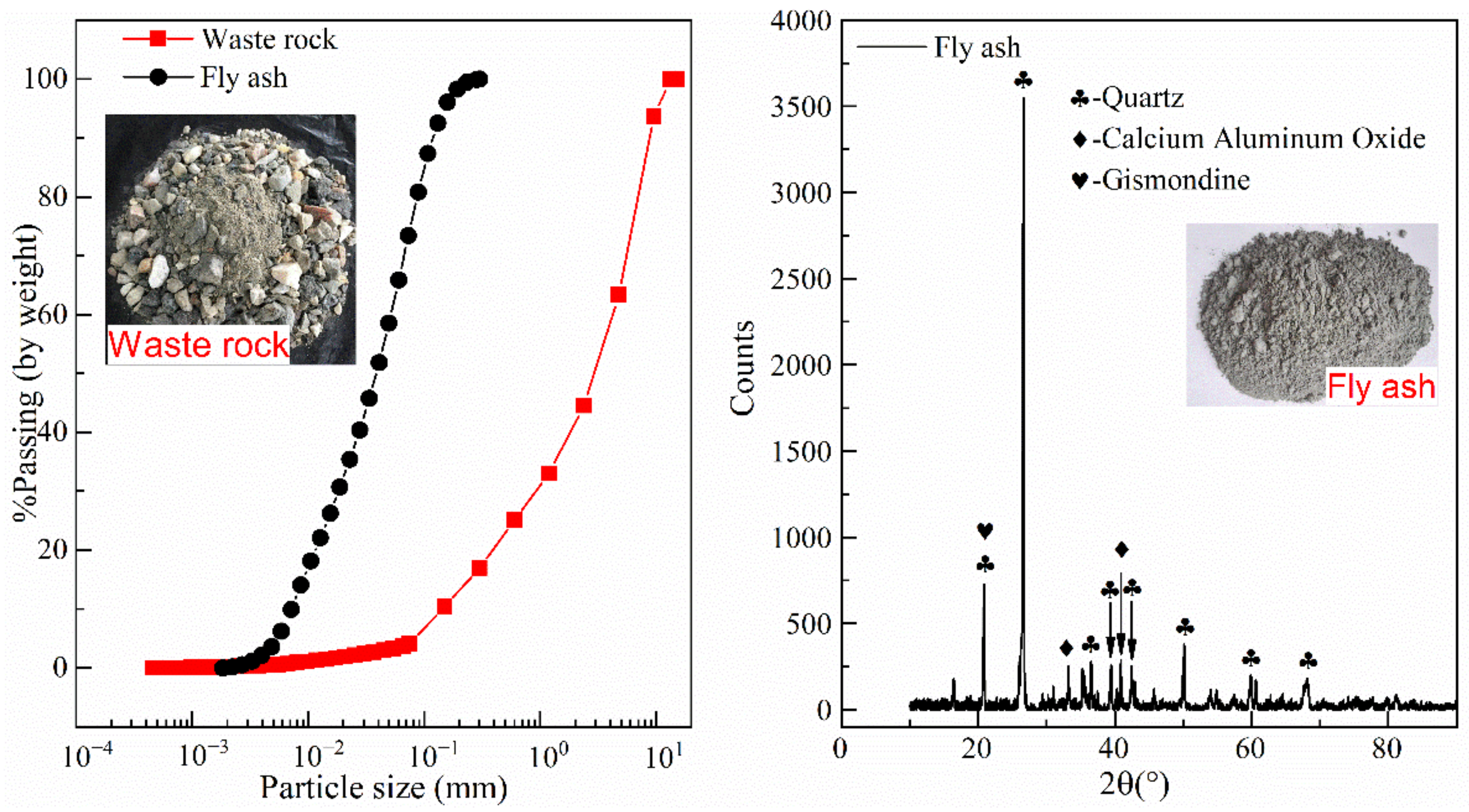
The test materials, including aggregates (waste rock and fly ash), were obtained from Jinchuan Nickel Mine, and the binder material was 42.5# OPC from Jinni Group in Jinchang (China). The waste rock was well-graded sand with traces of silt and pebbles, which is the useless rock generated during the drafting or driving procedure. The fly-ash was collected directly from a local thermal power plant where electrostatic filters are used.
To give a brief engineering background, the Jinchuan Nickel Mine, located in Gansu Province of Western China, is the third largest copper–nickel sulfide deposit in the world. The geological conditions for deposit include fragmented ore rock, developed joint fissures, and high in-situ stress. The current mining operation is over 1000 m beneath the surface, where the cemented undercut- and-fill mining method has been adopted. Tailings backfilling in Jinchuan Nickel Mine is administratively prohibited because some rare metals cannot be extracted currently (technical and economic limitations). Therefore, tailings are reserved for future recycling and waste rock and sand are used for backfill.
2.1.1. Material Physical and Chemical Properties
The physicochemical properties of the materials were analyzed, and the results of the main chemical compositions can be seen in Table 1. The density of the waste rock is 2.87 g/cm3, the specific weight in loose packing is 1.59 g/cm3, the porosity is 40.1%, and the mud content is 15.05%. In comparison, the density of the fly ash is 2.20 g/cm3, the specific weight in loose packing is 0.74 g/cm3, and the porosity is 59.7%.
2.1.2. Aggregate Particle Size Distribution
The mix proportion and properties of the filling slurry are closely related to the aggregate and its particle size distribution (PSD). In this section, aggregate screening tests were conducted using standard sieves for particles >75 μm in diameter and laser diffraction analysis for the finer parts. The results were combined to obtain the entire PSD (see Figure 1). The featured particle parameters are shown in Table 2. The low-quality fly ash has relatively coarser particles, which may be related to the power plant’s collection devices, and can be classified as lower than grade III according to the Chinese national standard of GB/T 1596-2017.
2.2. Tests
2.2.1. Slump and Slump Flow
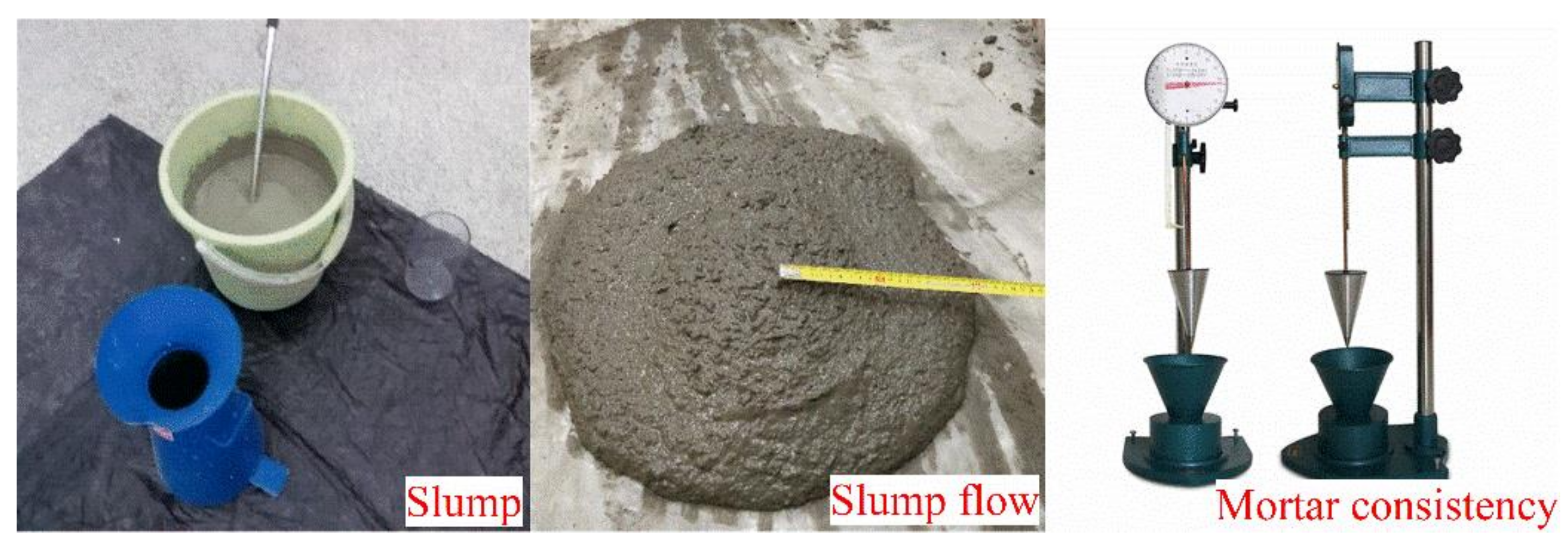
The mechanical meaning of slump (S) is the amount of deformation caused by the internal resistance when the slurry loses its external force and begins to flow under the action of self-weight [16]. It is generally accepted that the slurry can be gravity-fed when the slump is 23–27 cm [17,18]. A slump test was performed in accordance with the American Society for Testing Materials (ASTM) Standard C143. The slump flow (SF) is a corresponding index to the slump. The slump cannot reflect the accurate state when S > 23 cm, so the average diameter of the slump collapse is used as a substitution, i.e., the slump flow. The slump flow is measured with a tape (see Figure 2). The test for each specimen was repeated twice to ensure the repeatability of the results, and the mean value was used.
2.2.2. Mortar Consistency
The mortar consistency (MC) is used to determine the mobility of mortar. Since mortar is a type of paste, the MC can reflect the flow performance of the backfill slurry. It is measured using a mortar consistometer, which shows the sinking depth of the cone in the apparatus filled with slurry. To perform the test, pour the slurry into the cone of the consistency meter, and make sure the slurry surface is about 10 mm lower than the upper surface of the container. Then, adjust the drop cone’s initial position so that its tip is suspended on the slurry surface and record the initial reading of the dial. Finally, open the brake screw to let the cone fall into the slurry, read the sinking cone depth within 10 s. The reading difference is the measured consistency. The procedure follows the Chinese industry standard of JGJVT70-2009. Each specimen was tested twice for accuracy and repeatability.
2.2.3. Layering Degree
The layering degree (LD) is a stability index of cement mortar and can represent the segregation of the slurry. It is caused by the relative movement of the solid particles in the slurry, which forms a concentration gradient on the vertical plane [18]. The coursing degree is measured based on the mortar consistency test. This is the difference in MC between the original MC and that of the lower half in the measuring cylinder barrel being silent for a period of time. The layering degree test was also performed according to JGJVT70-2009. Each specimen was tested twice.
2.2.4. Bleeding Rate
The bleeding rate (BR) is pressure-free and used to indicate the capacity of water retention. It is the ratio of the bleeding water from the slurry to the total water content of the slurry after it has settled for 30 min. It is beneficial for proper bleeding in pipeline transportation, which lubricates the particles. However, problems of losing flowing capacity will occur when the BR is too large. The bleeding rate test was performed under the procedure of ASTM C232/C232M). Each specimen was measured three times for accuracy and repeatability.
3. Test Results and Analysis
3.1. Test Results
The flow property test results of the fly ash-waste rock mixed-aggregate filling slurry are shown in Table 3, according to the above methods and scheme.
3.2. Analysis
3.2.1. Variation in Slump
From Table 3, the effects of the fly ash proportion, binder content, and solid mass concentration on the slump are shown in Figure 3. Figure 3a shows the relation between the average slump and the fly ash proportion, which is not significant. This is the situation when the slump is >23 cm, as previously mentioned. Figure 3b shows the same relations but differs in concentration of Cw. Similar conclusions can be inferred when Cw is <81%, but the slump linearly (F = 176.76 > F(0.05,1,3) = 10.13) decreases with the addition of fly ash when the concentration reaches 81%. This phenomenon indicates that there is a qualitative change in slurry properties, meaning that it can be considered a homogeneous flow. The effect of fly ash on the slump should be considered together with concentration. In a homogeneous flow the free water is relatively less. The pore structure created by the large content of fly ash absorbs a lot of water; thus, the particle friction and slurry viscosity are increased, resulting in a poor fluidity (lower slump).
3.2.2. Variation of Slump Flow
The slump flow is used instead when the slump is greater than 23 cm. Figure 4 shows the typical variations in the slump flow with the fly ash addition at different solid percentages and binder contents.
On average, the slump flow is negatively correlated with the added amount of fly ash, as shown in Figure 4a, and a fitting line is provided (F = 15.21 > F(0.05,1,3) = 10.13). Therefore, the substitution of slump flow is more reasonable. Specifically, three similar fitting lines for different solid mass concentrations Cw can be deduced, as shown in Figure 4b. The relations can be formed in Equation (1). For SF77%, the F-test showed the results were insignificant, mainly due to only three samples being used, while R2 is acceptable
where SFi = slump flow with the concentration i; x = added proportion of fly ash.
For different binder contents, as shown in Figure 4c, the quantitative relations are not obvious. The effect of the binder content on the slump flow is relatively smaller than those of the fly ash proportion and concentration. However, the slump and slump flow are mutually reinforcing. A fitting line is provided when the slump is >23 cm, as shown in Figure 4d, and the relation is illustrated in Equation (2)
where SF = slump flow; S = slump.
3.2.3. Variation in the Mortar Consistency and Layering Degree
Figure 5 shows the typical variations in the mortar consistency and layering degree with different fly ash proportions and various binder contents Bw and concentrations Cw. The fittings in Figure 5a,b are insignificant, with R2 = 0.6 and F = 4.55 > F(0.05,1,3) = 10.13. This is mainly due to the experimental error. The awl of the testing instrument can hit the coarse particles when it drops in the test, because the maximum particle in the slurry is 12 mm in diameter, and the consistometer is conical in shape. This issue can also occur in the layering degree test, and the results are shown in Figure 5c,d. The average layering dress fluctuates with different fly ash amounts. It is a watershed when the concentration is 77% from the curve trend, which indicates that the slurry state has changed.
3.2.4. Variation of the Bleeding Rate
Figure 6 shows the variation in the bleeding rate with different amounts of fly ash, binder contents, and concentrations. The average bleeding rate gradually decreases with the increase in fly ash content, as shown in Figure 6a. Particularly, the BR remains practically constant when the fly ash proportion exceeds 30%. This is because the slurry has become a homogeneous flow. Therefore, the appropriate number of fine particles can enhance water retention and improve the stability of the slurry. In Figure 6b, the bleeding rate changes in compliance with the above average description for different solid concentrations Cw. However, when Cw is 81%, BR < 9% in all ranges of fly ash proportion, this implies that the slurry has become a homogeneous flow, and this explains the mutations in Figure 5d. The bleeding rate when Cw = 79% shows a negative exponential correlation with the amount of fly ash, as shown in Equation (3)
where BRi = Bleeding rate of the slurry when the solid concentration is i; x = fly ash proportion.
4. Principal Component Analysis of the Flow Properties
4.1. Questions
The effects of the solid mass concentration, binder content, and fly ash addition on the flow properties are obtained from the above analysis. Some of these parameters are related to one another; some parameters can be used to characterize the same feature; some parameters are affected by unavoidable errors in the test process. Noticeably, there is a question in the utilization: which indicators are more critical, and which can be used to indicate the intrinsic properties of the slurry?
Mathematically, the question is how to eliminate the repetitive features and regroup the parameters into fewer, unrelated indicators. The principal component analysis is a statistical method used to solve this problem.
4.2. Principal Component Analysis
- (1)
- Parameter determination and data normalization matrix Z
In this case, the parameters involved are the five slurry flow properties discussed above. All groups in Table 3 are data samples which form the initial data matrix X = (xij)17 × 5. The initial data are normalized using Equation (4) to obtain the standardized initial data matrix Z = (zij)17 × 5
where = mean value of variable j; = standard deviation of variable j; i = 1, 2, …, 17 (number of samples); j = 1, 2, …, 5 (number of variables).
- (2)
- Calculating the correlation coefficient matrix R
From the standardized initial data matrix Z, the correlation coefficient matrix R = (rjk)5 × 5 can be calculated using Equation (5)
where n = number of samples (17); j = 1, 2, …, 5; k = 1, 2, …, 5.
- (3)
- Solving the load matrix A
From the obtained matrix R, the characteristic equation |R−λi = 0| can be solved to obtain its eigenvalues, and the eigenvalues greater than 1 are selected. In this case, there are two of them: λ1 = 2.835, and λ2 = 1.192. The cumulative variance contribution rate is 80.537%. Thus, two principal components (common factors) can be extracted. The corresponding eigenvector can be calculated as αj, λi. Load matrix A can be calculated according to conversion Equation (6).
where j = 1, 2, …,5; i = 1, 2. In this case,
- (4)
- Rotation factors
To maximize the difference among the common factors, a coordinate transformation of the road matrix A is required, which is called the rotation factor. In particular, we find the orthogonal matrix and make the load matrix after rotation , where the square element of each column has the greatest variance, which is max(V1 + V2), where V1 is the variance in , and is the variance in . In this case, the load matrix after the rotation is:
- (5)
- Factor score
Finally, referring to the initial problem, the new indicators (principal component F1, F2) are obtained to characterize the original five parameters from the equation F = CZ, where C is the factor score matrix in Equation (7)
where C = factor score matrix; A1 = load matrix after rotation; R = correlation coefficient matrix.
The expressions of the two new indicators (principal components) are
where zi = the i variable in the initial normalized data. Thus, by simplifying to two indicators, they can be used for clustering, discrimination, and other analysis.
4.3. Application of the New Indicators
From the new indices in Equation (8), we substitute the data from the normalized initial data matrix Z= (zij)17 × 5 and obtain the factor scores of the 17 groups of different slurries in Table 4.
From Table 4, the flowing conclusions can be inferred:
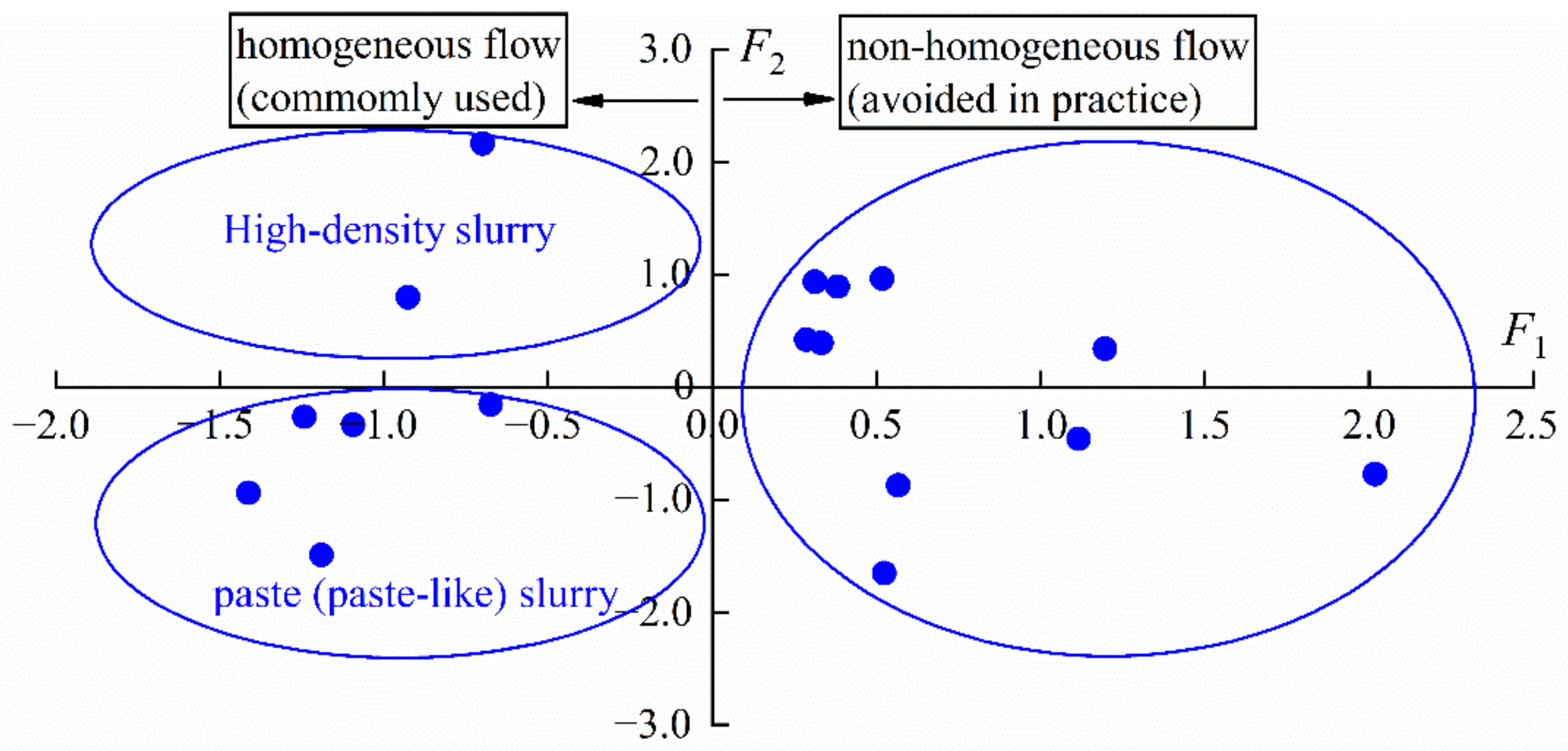
- (1)
- For the F1 > 0 groups (A1, A2, A3, A4, A6, B1, B2, B3, and B5, whereas B7 is misjudged), the bleeding rates are larger than 8%. These groups of slurries cannot satisfy the requirements of a quasi-homogeneous flow. They easily aggravate pipe wear, can cause blockage accidents during pipeline transport, can affect the overall stability of the filling body and endanger mining safety;
- (2)
- For the F1 < 0 and F2 < 0 groups (A5, A7, B4, B6, B8), Table 3 shows that these slurries have a slump value of 15–26 cm and a bleeding rate of 1–6.5%, which generally conforms to the identifications of paste or paste-like slurry proposed by Wu Aixiang’s definition;
- (3)
- For the F1 < 0 and F2 > 0 groups, Table 3 and the observation in the test process, show that these groups are high-density slurries, which is another widely used slurry configuration.
The indices F1 and F2 can be used to identify the slurry category. If we regard F1 as the x-axis and F2 as the y-axis, the slurries in the 1st and 4th quadrants are easy to delaminate, which should be avoided in practice. The slurry in the 2nd quadrant is high-density slurry. The slurry in the 3rd quadrant is a paste or paste-like slurry, as shown in Figure 7.
4.4. Verification
When identifying a slurry flow of a general mining operation, the proposed simple five flow properties are tested first, then the values are substituted into Equations (4) and (8), obtaining the F1 and F2 indices. Finally, the slurry flow can be identified from Figure 7.
To verify the method, another practical iron tailing backfill was applied. The iron tailings were obtained from Dazhong Iron Ore in Inner Mongolia of China. The tailings’ grain-size characteristics, slurry configuration parameters, and slurry flow test results are listed in Table 5.
The five flow test results were processed by Equations (4) and (8), obtaining the (F1, F2) of the tailings backfill (−0.215, −2.437). The calculated (F1, F2) correctly indicates a paste (paste-like) slurry, which is in agreement with the site practice.
5. Conclusions
The property test of fly ash-waste rock mixed-backfilling slurry shows the effects of the slurry concentration, binder content, and fly ash addition on the slump, slump flow, mortar consistency, layering degree, and bleeding rate. The slump test result shows that the relationships are hidden when the slump is greater than 23 cm; in this case, the slump flow is a substitution, which shows the negative relation to the fly ash content at different concentrations.
The bleeding rate gradually decreases with the increase in fly ash content, and a negative exponential fitting curve is obtained. The BR remains practically constant when the fly ash proportion exceeds 30%, which indicates that the slurry has become a homogeneous flow.
The principal component analysis method was applied to simplify and explain the use of flow properties. In this case, two new indices, F1 and F2 are deduced, which can be used to identify the slurry category: slurries with F1 > 0 are easy to delaminate and should be avoided in practice, whereas F1 < 0 indicates a homogeneous flow (or quasi-homogeneous flow). In detail, F1 < 0 and F2 > 0 indicates a high-density slurry, and F1 < 0 and F2 < 0 indicates a paste (paste-like) slurry, both of which are commonly used in practice.
Author Contributions
Conceptualization, H.W. and B.X.; Data curation, Q.G.; Formal analysis, B.X.; Funding acquisition, Q.G.; Investigation, H.W.; Methodology, B.X.; Project administration, Q.G.; Resources, Q.G.; Software, H.W.; Supervision, Q.G.; Validation, B.X. and Q.G.; Visualization, H.W. and B.X.; Writing—review & editing, B.X. All authors have read and agreed to the published version of the manuscript.
Funding
This research and the APA were funded by Hebei Province Science and Technology Support Program (CN), Grant number 19073818Z.
Data Availability Statement
The data is all presented within this article. No new data were created or analyzed in this study. Data sharing is not applicable to this article.
Acknowledgments
The authors are grateful for the help and support of Longshou Mine, Jinchuan Group Co. LTD. for offering the materials.
Conflicts of Interest
The authors declare no conflict of interest. The funders had no role in the design of the study; in the collection, analyses, or interpretation of data; in the writing of the manuscript, or in the decision to publish the results.
References
- Panchal, S.; Deb, D.; Sreenivas, T. Mill tailings based composites as paste backfill in mines of U-bearing dolomitic limestone ore. J. Rock Mech. Geotech. Eng. 2018, 10, 310–322. [Google Scholar] [CrossRef]
- Chen, Q.; Zhang, Q.; Fourie, A.; Xin, C. Utilization of phosphogypsum and phosphate tailings for cemented paste backfill. J. Environ. Manag. 2017, 201, 19–27. [Google Scholar] [CrossRef] [PubMed]
- Ouattara, D.; Belem, T.; Mbonimpa, M.; Yahia, S. Effect of superplasti-cizers on the consistency and unconfined compressive strength of cemented paste backfills. Constr. Build. Mater. 2018, 181, 59–72. [Google Scholar] [CrossRef]
- Zhang, X.; Qiao, D. Simulation and experiment of pipeline transporta-tion of high density filling slurry with coarse aggregates. Chin. J. Nonferrous Met. 2015, 25, 258–266. [Google Scholar]
- Li, A.; Cao, S.; Liu, H.; Sun, W.; Lu, Y. Critical flow rate for slurry pipeline transportation. Min. Metall. Eng. 2016, 36, 26–29. [Google Scholar]
- Wasp, E.J.; Kenny, J.P.; Gandhi, R.L. Solid-liquid flow slurry pipeline transportation [Pumps, valves, mechanical equipment, economics]. Ser. Bulk Mater. Handl. 1997, 1, 102–184. [Google Scholar]
- Chen, W.; Gu, D.; Gao, Q. Criterion of high concentration slurry and its laminar flow transport characteristics. Chin. J. Nonferrous Met. 1995, 5, 35–39. [Google Scholar]
- Fall, M.; Célestin, J.; Sen, H.F. Potential use of densified polymer-pastefill mixture as waste containment barrier materials. Waste Manag. 2010, 30, 2570–2578. [Google Scholar] [CrossRef] [PubMed]
- Sun, H.; Jie, H.; Liu, W.; Huang, Y.; Yang, B. Analysis of characteristic pa-rameters of self-flowing pastefill systems. Nonferrous Met. 2000, 52, 7–10. [Google Scholar]
- Zhang, L.; Zhang, J.; Hassani, F.P.; Zhang, X. Slump tests for yield stress of paste tailings. Met. Mine 2017, 1, 30–36. [Google Scholar]
- Li, X.; Du, J.; Gao, L.; He, S.; Gan, L.; Sun, C.; Shi, Y. Immobilization of phosphogypsum for cemented paste backfill and its environmental effect. J. Clean. Prod. 2017, 156, 137–146. [Google Scholar] [CrossRef]
- Wu, A.; Wang, H. Theory and Technology of Paste Filling in Metal Mine; Science Press: Beijing, China, 2015; pp. 35–79. [Google Scholar]
- Koohestani, B.; Darban, A.K.; Mokhtari, P. A comparison between the in-fluence of superplasticizer and organosilanes on different properties of cemented paste backfill. Constr. Build. Mater. 2018, 173, 180–188. [Google Scholar] [CrossRef]
- Panchal, S.; Deb, D.; Sreenivas, T. Variability in rheology of cemented paste backfill with hydration age, binder and superplasticizer dosages. Adv. Powder Technol. 2018, 29, 2211–2220. [Google Scholar] [CrossRef]
- Mangane, M.B.C.; Argane, R.; Trauchessec, T.; Lecomte, A.; Benzaazoua, M. Influence of superplasticizers on mechanical properties and workability of cemented paste backfill. Miner. Eng. 2018, 116, 3–14. [Google Scholar] [CrossRef]
- Yang, Y.L.; Du, Y.J.; Reddy, K.R.; Fan, R.D. Phosphate-amended sand/Ca-bentonite mixtures as slurry trench wall backfills: Assess-ment of workability, compressibility and hydraulic conductivity. Appl. Clay Sci. 2016, 142, 120–127. [Google Scholar] [CrossRef]
- Ma, K.; Feng, J.; Long, G.; Xie, Y.; Chen, X. Improved mix design method of self-compacting concrete based on coarse aggregate average diame-ter and slump flow. Constr. Build. Mater. 2017, 143, 566–573. [Google Scholar] [CrossRef]
- Creber, K.; Mcguinness, M.; Kermani, M.F.; Hassani, F.P. Investigation into changes in pastefill properties during pipeline transport. Int. J. Miner. Process. 2017, 163, 35–44. [Google Scholar] [CrossRef]
Figure 1.
PSD, appearance, and XRD patterns of waste rock and fly ash.

Figure 2.
Slump and slump flow measurement.

Figure 3.
Variation of the slump with the fly ash addition: (a) average slump; (b) slumps with varying concentrations.
Figure 3.
Variation of the slump with the fly ash addition: (a) average slump; (b) slumps with varying concentrations.

Figure 4.
Variation of SF with the fly ash addition at different solid percentages and binder contents: (a) average SF vs. fly ash content; (b) SF at varying concentrations vs. fly ash content; (c) SF at varies binder content vs. fly ash content; (d) average SF vs. average S.
Figure 4.
Variation of SF with the fly ash addition at different solid percentages and binder contents: (a) average SF vs. fly ash content; (b) SF at varying concentrations vs. fly ash content; (c) SF at varies binder content vs. fly ash content; (d) average SF vs. average S.

Figure 5.
Variation in the mortar consistency and layering degree: (a) average MC vs. fly ash content; (b) MC at varying concentrations vs. fly ash content; (c) average LD vs. fly ash content; (d) LD at varying concentrations vs. fly ash content.
Figure 5.
Variation in the mortar consistency and layering degree: (a) average MC vs. fly ash content; (b) MC at varying concentrations vs. fly ash content; (c) average LD vs. fly ash content; (d) LD at varying concentrations vs. fly ash content.

Figure 6.
Relations between the BR and the fly ash content: (a) average BR; (b) BR at varying concentrations.
Figure 6.
Relations between the BR and the fly ash content: (a) average BR; (b) BR at varying concentrations.

Figure 7.
Identification of the new indices for the slurry flow.


Table 1.
Main chemical compositions of the waste rock and fly ash.
| Compositions | SiO2 | Al2O3 | CaO | MgO | Fe2O3 | TiO2 | P2O5 | K2O | Na2O | Cr2O3 | SO3 | PbO | NiO |
|---|---|---|---|---|---|---|---|---|---|---|---|---|---|
| Waste rock/% | 36.31 | 3.39 | 3.86 | 28.15 | 16.32 | 0.02 | - | 0.24 | 0.03 | 0.01 | 0.23 | 0.02 | 0.20 |
| Fly ash/% | 38.38 | 19.57 | 3.13 | 0.82 | 22.91 | 1.23 | 0.64 | 0.64 | 0.97 | 0.01 | 1.87 | 0.14 | - |
Table 2.
Featured particle parameters of the mixed aggregate.
| Fly Ash Proportion | d10/μm | d30/μm | d50/μm | d60/μm | d90/μm | dav/μm | d95/μm | Cu | Cc | Index n |
|---|---|---|---|---|---|---|---|---|---|---|
| 0% | 143.2 | 926.2 | 2993.6 | 4281.8 | 8897.1 | 2711.2 | 10,209 | 29.9 | 1.4 | 0.56 |
| 15% | 37 | 320.1 | 1983.6 | 3357.4 | 8608 | 2310 | 9731.5 | 90.7 | 0.8 | 0.43 |
| 20% | 26.4 | 192 | 1602.3 | 2994.1 | 8486.5 | 2176.4 | 9538.5 | 113.4 | 0.5 | 0.38 |
| 25% | 19.5 | 109.7 | 1207.3 | 2598.5 | 8351.5 | 2042.7 | 9333.4 | 133.3 | 0.2 | 0.35 |
| 30% | 15.5 | 82.2 | 819.3 | 2167 | 8195.8 | 1909 | 9100.7 | 139.8 | 0.2 | 0.33 |
| 35% | 12.8 | 73.6 | 501.1 | 1699.9 | 8016.7 | 1775.3 | 8842.5 | 132.8 | 0.2 | 0.31 |
| 100% | 2.7 | 15.8 | 35.5 | 47.5 | 109.2 | 46.2 | 131.5 | 17.6 | 1.9 | 0.57 |
Table 3.
Scheme and results of the slurry flow property tests.
| Scheme | Results | |||||||
|---|---|---|---|---|---|---|---|---|
| No. | Fw/% | Bw/(kg m3) | Cw/% | S/cm | SF/cm | MC/cm | LD/cm | BR/% |
| A1 | 15 | 270 | 77 | 24.8 | 87.5 | 12.25 | 2.5 | 18.76 |
| A2 | 15 | 290 | 79 | 25.5 | 82 | 11.8 | 2.7 | 12.57 |
| A3 | 15 | 310 | 81 | 23.7 | 66 | 11.6 | 3.8 | 8.7 |
| A4 | 25 | 270 | 79 | 28 | 75 | 11.35 | 2.95 | 9.42 |
| A5 | 25 | 290 | 81 | 25.6 | 54 | 9.5 | 3.25 | 5.5 |
| A6 | 25 | 310 | 77 | 28 | 76 | 11.9 | 1.8 | 10.52 |
| A7 | 35 | 270 | 81 | 24.5 | 42 | 9.9 | 3.65 | 3.74 |
| A8 | 35 | 290 | 77 | 28.5 | 71 | 10.5 | 0.5 | 7.49 |
| A9 | 35 | 310 | 79 | 27.5 | 54 | 10.85 | 2.2 | 5.27 |
| B1 | 20 | 290 | 79 | 27.5 | 69 | 11.8 | 2.3 | 20.41 |
| B2 | 20 | 290 | 81 | 27.7 | 65 | 11.9 | 1.6 | 11.8 |
| B3 | 20 | 310 | 79 | 27.5 | 75 | 11.6 | 1.7 | 10.52 |
| B4 | 20 | 310 | 81 | 25.2 | 56 | 10.65 | 2.45 | 6.18 |
| B5 | 30 | 290 | 79 | 27.3 | 64 | 12.5 | 2.25 | 7.82 |
| B6 | 30 | 290 | 81 | 25.5 | 46 | 10.65 | 3 | 4.03 |
| B7 | 30 | 310 | 79 | 27 | 64 | 12.9 | 4.25 | 5.32 |
| B8 | 30 | 310 | 81 | 24.2 | 42 | 10.2 | 4.35 | 3.52 |
Table 4.
Factor scores of different slurries.
| No. | A1 | A2 | A3 | A4 | A5 | A6 | A7 | A8 | A9 |
|---|---|---|---|---|---|---|---|---|---|
| F1 | 2.018 | 1.115 | 0.523 | 0.286 | −1.242 | 0.517 | −1.414 | −0.700 | −0.927 |
| F2 | −0.773 | −0.459 | −1.653 | 0.425 | −0.263 | 0.969 | −0.937 | 2.165 | 0.801 |
| NO. | B1 | B2 | B3 | B4 | B5 | B6 | B7 | B8 | |
| F1 | 1.195 | 0.312 | 0.381 | −0.675 | 0.332 | −1.094 | 0.565 | −1.190 | |
| F2 | 0.345 | 0.940 | 0.893 | −0.154 | 0.394 | −0.331 | −0.872 | −1.489 |
Table 5.
Tailings grain size characteristics, slurry configuration parameters, and flow test results in the Dazhong site.
Table 5.
Tailings grain size characteristics, slurry configuration parameters, and flow test results in the Dazhong site.
| d10/mm | d30/mm | d50/mm | d60/mm | Cement Content/% | Cw/% | S/cm | SF/cm | MC/cm | LD/cm | BR/cm |
|---|---|---|---|---|---|---|---|---|---|---|
| 0.083 | 0.139 | 0.245 | 0.273 | 20 | 70 | 22.2 | 77 | 8.7 | 5.1 | 8.5 |
Publisher’s Note: MDPI stays neutral with regard to jurisdictional claims in published maps and institutional affiliations. |
© 2021 by the authors. Licensee MDPI, Basel, Switzerland. This article is an open access article distributed under the terms and conditions of the Creative Commons Attribution (CC BY) license (https://creativecommons.org/licenses/by/4.0/).
Share and Cite
MDPI and ACS Style
Wei, H.; Xiao, B.; Gao, Q. Flow Properties Analysis and Identification of a Fly Ash-Waste Rock Mixed Backfilling Slurry. Minerals 2021, 11, 576. https://0-doi-org.brum.beds.ac.uk/10.3390/min11060576
AMA Style
Wei H, Xiao B, Gao Q. Flow Properties Analysis and Identification of a Fly Ash-Waste Rock Mixed Backfilling Slurry. Minerals. 2021; 11(6):576. https://0-doi-org.brum.beds.ac.uk/10.3390/min11060576
Chicago/Turabian StyleWei, Hanbo, Bolin Xiao, and Qian Gao. 2021. "Flow Properties Analysis and Identification of a Fly Ash-Waste Rock Mixed Backfilling Slurry" Minerals 11, no. 6: 576. https://0-doi-org.brum.beds.ac.uk/10.3390/min11060576
Note that from the first issue of 2016, this journal uses article numbers instead of page numbers. See further details here.