
Full-Scale Simulation and Validation of Wear for a Mining Rope Shovel Bucket


1
Division of Solid Mechanics, Luleå University of Technology, 97187 Luleå, Sweden
2
Boliden Mines, 98292 Sakajärvi, Sweden
3
Boliden Mines, 93632 Boliden, Sweden
*
Author to whom correspondence should be addressed.
Minerals 2021, 11(6), 623; https://0-doi-org.brum.beds.ac.uk/10.3390/min11060623
Submission received: 30 April 2021
/
Revised: 8 June 2021
/
Accepted: 8 June 2021
/
Published: 11 June 2021
(This article belongs to the Special Issue Simulation Using the Discrete Element Method (DEM) in the Minerals Industry)
Abstract
:Failure in industrial processes is often related to wear and can cause significant problems. It is estimated that approximately 1–4% of the gross national product for an industrialized nation is related to abrasive wear. This work aims to numerically predict development of wear for full-scale mining applications in harsh sub-arctic conditions. The purpose is to increase the understanding of wear development in industrial processes and optimize service life and minimize costs related to wear. In the present paper, a granular material model consisting of the discrete element method (DEM) and rigid finite element particles is utilized to study wear in full-scale mining applications where granular materials and steel structures are present. A wear model with the basis in Finnie’s wear model is developed to calculate wear from combined abrasive sliding and impact wear. Novel in situ full-scale experiments are presented for calibration of the wear model. A simulation model of the rope shovel loading process is set up where the bucket filling process is simulated several times, and the wear is calculated with the calibrated wear model. From the full-scale validation, it is shown that the simulated wear is in excellent agreement when compared to the experiments, both regarding wear locations and magnitudes. After validation, the model is utilized to study if wear can be minimized by making small changes to the bucket. One major conclusion from the work is that the presented wear simulator is a suitable tool that can be used for product development and optimization of the loading process.
Keywords:
mining; simulation; discrete element method; DEM; full-scale; wear; validation; mining equipment1. Introduction
Wear occurs in all processes where materials or components come into contact with each other. In the mining industry, wear can account for up to 50% of the total maintenance cost [1]. According to [2], the cost of abrasive wear has been estimated to range from 1% to 4% of the gross national product of an industrialized nation. Granular material handling is a critical process in the mining industry. The ore that is extracted from the rock is handled at all stages, from blasting to crushing and grinding. In the loading process, large rope shovels of up to 1500 tons in weight loads blasted ore and waste rock to haul trucks. In this process, problems related to wear often occur. The buckets of these enormous machines can load up to 120 tons of fragmented rocks. The material turnover is approximately 30–70 kton per day in the Boliden open-pit copper mine Aitik, located 20 km outside of Gällivare in Northern Sweden. The part on the rope shovel and other loading machinery that is in direct contact with the granular material is the bucket. Due to the large material turnover and the harsh conditions that the buckets are subjected to, the buckets are often the cause for both planned and unexpected machine downtime.
Costs related to bucket wear and ground engaging tools (GET) are one of the primary cost drivers in operating a rope shovel. Replacing a dipper is an investment in the order of 1–1.5M USD, and the annual GET consumption is around 300k USD. This means that the cost of the bucket and wear parts are larger than the operator cost for the shovel. In addition, bucket-related downtime cost can be significant, especially related to unplanned failures. Hence, to extend the service life of buckets and to better plan the maintenance, a better understanding of wear and how to minimize it is of fundamental importance.
Prediction of wear has been an active field of research for decades; however, wear is not yet fully understood. Several researchers have stated that there only exists four wear mechanisms [3,4], namely abrasive wear, adhesive wear, wear by contact fatigue, and corrosive (or tribo-oxide) wear. Wear processes are described by one or a combination of the four possible wear mechanisms and are related to how the contact occurs. During the 1950s and 1960s, some of the most fundamental work was conducted regarding the understanding and prediction of wear. A seminal work on wear prediction was presented by Archard in 1953 [5]. From studying experiments on two bodies having contact, Archard revealed that the contact area was increasing with applied load. He also observed that the material removal was proportional to the normal contact force and sliding distance, and inversely proportional to the hardness of the material. Archard’s wear law has often been used for the prediction of wear in many applications. In 1958, the Rabinowicz criterion for adhesive wear was formulated [6]. He concluded that, what determines if a particle/fragment will become a worn particle or not depends on if the elastic energy stored in the particle/fragment exceeds the adhesive energy at the point of attachment. The result from the paper was a criterion to calculate the size of worn particles. This criterion has been proven to be accurate in recent research where adhesive wear was studied at micro-level [7]. In 1960, Finnie [8] developed an energy-based wear model for erosive wear based on hard particles impacting ductile metal plates at certain angles of impact. Erosive wear is described as the wear from a solid surface in contact with a stream of particle impacts. The model is dependent on impact angle, mass, and velocity of particles, amount of particles, and contact properties between particles and surface. Magnée [9] developed a generalized law of erosive wear. The model is based on the work by Finnie [8] and Bitter [10] and combines hardness and particle sharpness. Even though the intent was to create a generalized wear law, the author did not present any application of the model. Since its formulation, the Magnée wear law has received some attention and has been implemented for simulation of wear for computational fluid dynamics [11]. A shear impact energy model (SIEM) used for erosion was proposed by Zhao et al. [12]. The background for the model was from previous work [13], where it was shown that the shear impact energy showed a good correlation to the wear volume for different impact angles. Through numerical modeling, the authors demonstrated that 1/4 of the shear impact energy is converted to erosive energy. It was concluded that the shear impact energy is a suitable measure for predicting wear. The model was validated against experimental results and showed good potential.
In the study of industrial granular material flows, the use of numerical methods has increased rapidly in the last decade. As of 2021, most of the major companies dealing with bulk material handling utilize numerical models for granular material in one way or another. The discrete element method (DEM) is by far the most common approach when modeling granular materials. The method was introduced by Cundall and Strack in 1971 [14] and 1979 [15]. Since then, the method has been developed continuously, while at the same time the computational capacities have significantly improved. This development has enabled detailed simulations including almost a billion particles [16]. DEM is also a very common method when dealing with different mining applications [17], such as grinding [18,19,20] and crushing [21]. Recently, wear phenomena have been investigated using DEM simulation. Roessler et al. [22] aimed to develop a standardized calibration procedure for abrasive sliding wear. An experimental setup where normal force and sliding distance could be varied was used. The mass and volume loss due to wear was experimentally measured. The same setup was modeled with DEM, and the Archard wear law was calibrated from the results of the experiment. The authors showed that the results from short simulations of a few seconds could be used to obtain the total volume and mass loss from time-consuming experiments. Ilic et al. [23] studied wear in transfer chutes for iron ore and aimed to develop a criterion for reducing wear in chutes. Wear was modeled by using shear and impact intensities in the DEM-structure contacts in order to evaluate different designs performance. DEM with multi-sphere particles was used to model abrasive wear on structural steel plates [24]. Perhaps most of the wear studies when it comes to granular materials are in the field of comminution, e.g., [19,25,26,27,28]. Boemer [29] gives a thorough review of the used wear models when it comes to liner wear in ball mills. In one study by Kalala [30], Archard’s wear law was calibrated and validated with the ASTM G65 experiment. Relative wear patterns showed good agreement with experimentally observed measurement when different particle sizes were examined. Continuous shearer machines for coal cutting and loading were simulated using DEM with the Archard wear model [31]. Jafari et al. [32] used DEM to investigate how wear in the screening process was affected by different process parameters. Further, Finnie’s wear model was used to investigate what parameters influence the impact wear [33]. It was concluded that the impact angle, impact speed, particle size, and particle density were the main influences on the amount of wear. It was also shown that the local wear depends on how a surface is discretized, i.e., the grid size. However, the total global wear remained consistent. Rojas et al. simulated wear using an Archard–DEM combination and showed a normalized wear difference on a dump truck body of less than 20% when compared to experiments [34]. Forström et al. used DEM-FEM and SPH-FEM to predict the wear on dump tipper bodies during unloading at full-scale [35,36]. A lab wear drum test was used to calibrate Archard’s wear law. Wear measurements were then performed on the truck body, and the experimental absolute wear was detected. Furthermore, the wear model was used to simulate the absolute wear. The conclusion from the paper was that an agreement in the relative wear map was seen. However, the absolute wear was not captured as intended.
From the studies presented in this section, most of the works have been performed on a smaller scale than the actual scale of the real application. Performing studies on smaller scales have many benefits, e.g., tests can be more controlled, better work environment, more precise test data, typically easily accessible and relatively cheap. On the other hand, full-scale experiments are less controllable, containing many influential parameters, are more expensive, and require in situ available data. Often, the results from down-scaled experiments gives reliable data and numerical models are accurately calibrated and validated to experiments. However, when the model is used for its actual industrial scale where different loads may exist, many simplifications must often be made to ensure realistic simulation times. Due to the simplifications and the different loads, it is not reasonable to automatically expect the model to capture the phenomenons occurring at full scale. For this reason, it is of importance to investigate if experimental and numerical full-scale approaches can give satisfactorily results, despite the mentioned drawbacks with the full-scale approach.
The objective of this work is to develop, calibrate and validate numerical models to enable the simulation of wear for full-scale mining applications. To fulfill the objective, full-scale experiments for calibrating an in-house wear model that is able to capture abrasive sliding and impact wear was developed. The wear was calculated on structural components and was coupled to a granular material model. The model was calibrated by using an in situ vibratory feeder that is used to feed rocks to a jaw crusher. Validation of the model was performed by comparing experimental and simulated wear from a rope shovel bucket. Finally, the model was utilized to investigate how small geometrical changes of a rope shovel bucket affects wear, dig forces, and bucket-filling degree.
2. Materials and Experiment
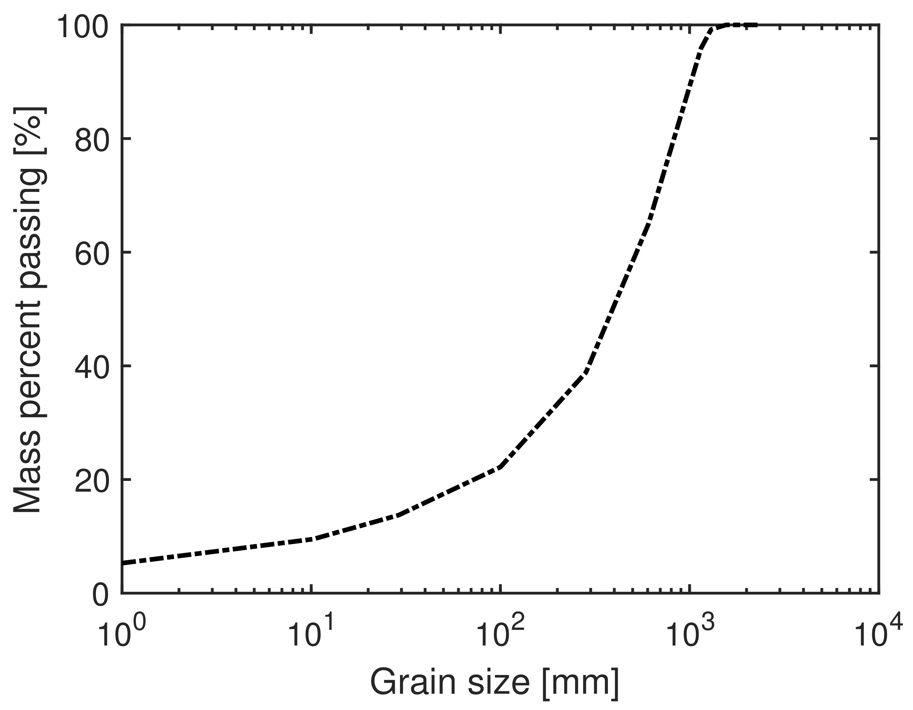
The small content of metal in the Aitik ore makes it difficult to distinguish ore from the waste rock on a bulk level. On the scales considered in the present study, it is thus assumed that the ore and waste rock can be treated as one granular material. The mineralogical composition of the rock types present in Aitik is dominated by quartz, plagioclase, K-feldspar, biotite, and muscovite. A particle size distribution (PSD) of the granular material is shown in Figure 1. The bulk density is between 1800 and 2000 kg/m, and the particle density is between 2600 and 2970 kg/m. The shapes of the rocks in the granular mass are mainly angular and blocky. The muck-pile generated by blasting is approximately 18 m high. After blasting, a few rocks were arbitrarily selected from the muck-pile and were 3D-scanned with a Leica RTC 360 3D scanner. The wear plates in the vibratory feeder are made of Hardox 450. The wear material of the rope shovel consists of mainly Hardox 500. The lip and teeth belonging to the bucket are of type Esco Ultralok System, and the material is cast steel of an unknown type.
2.1. Experimental Procedures
The experimental part of this work consists of two main parts. For full-scale calibration of a wear model, a vibratory feeder is used. The untreated material going into the vibratory feeder causes wear on metal plates. The second part of the experimental work consists of experiments for validation of the wear model. Experiments are performed on a rope shovel bucket with the same type of material and similar wear processes as the vibratory feeder experiment. Both of the experiments will be presented in this Section.
Vibratory Feeder
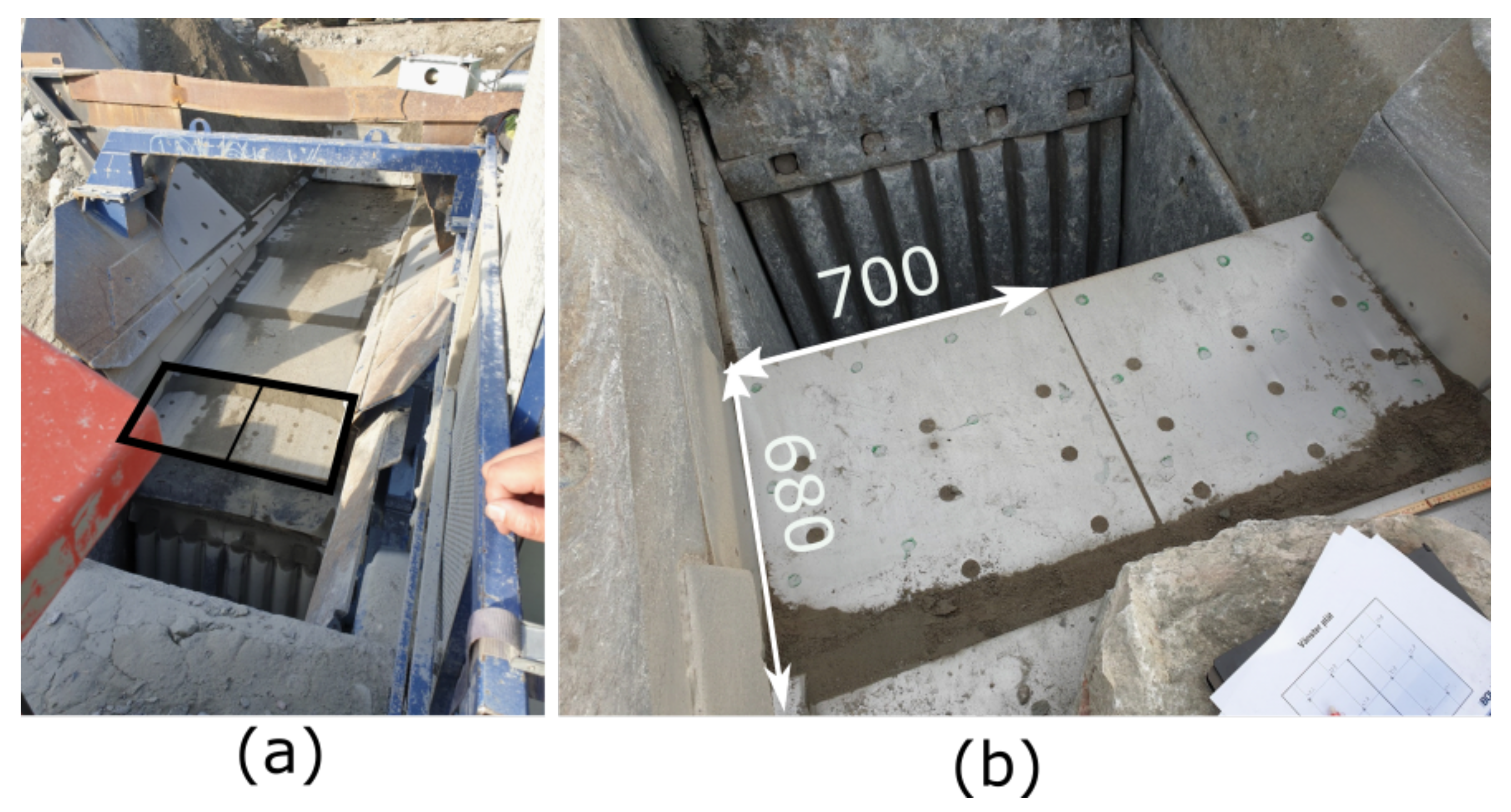
A vibratory feeder used to feed waste rock from the mine to a jaw crusher was used as a calibration case. In Figure 2a, the feeder is presented. The feeder is of type JF 1450 GBSd manufactured by P.J Jonsson and has a capacity of feeding 700 tonnes of rocks per hour. Drawings were provided from the manufacturer, although they are classified and not fully presented in this paper. The overall dimensions of the feeder are nonetheless presented in Figure 2b. Wheel loaders of type Volvo L-350 with buckets of approximately 8 m were used to load the feeder. The feeder is set on a spring table, and the vibration frequency ranged from 15 to 18 Hz at a 40° angle from the horizontal plane. The amplitude of the vibration was 3.5 mm. Video recording of when the material is filled into the feeder, as well as tonnage going through the feeder, was used to ensure that the simulation was behaving similarly to reality. Two steel plates of Hardox 450 were observed for wear, see Figure 3. Before the installation of brand new steel plates, the tonnage and operational hours were observed. The steel plates were measured on 12 different positions on each wear plate by using an ultrasonic thickness gauge. The thickness gauge was of type KARL DEUTSCH ECHOMETER 1075 Basic, with an accuracy of ±0.1 mm for plate thicknesses of 1.2–250 mm. Since both plates were measured, the total number of wear points was 24. A total of three separate measurement occasions were performed, excluding the initial thickness measurements of the plates. A template was made to make sure that identical positions on the plates were measured on every occasion.
2.2. Rope Shovel Wear Measurement
In a previous work by Svanberg et al. [38] the experimental setup for a rope shovel was presented in detail. In that study, the experimental work was related to rope shovel geometry, motions, and the granular material. In this study, the focus will be on describing the experimental procedure regarding wear measurements of the bucket.
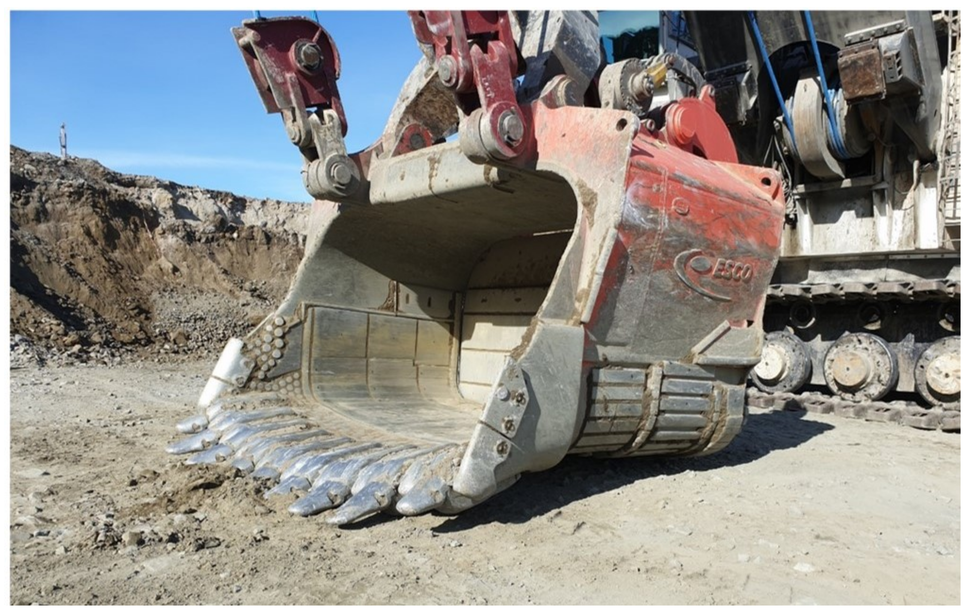
Buckets are the component of the shovels that are in direct contact with the material and are thus subjected to wear. One of the buckets in the Aitik mine is a 43 m large bucket belonging to a Bucyrus 495 electrical rope shovel (ERS), which can be seen in Figure 4. During a bucket filling cycle, the bucket is filled when penetrating and going through the muck-pile. After the bucket is filled, the door in the rear of the bucket is opened and the material is dumped into a haul truck. It has been observed that most of the wear during the filling stage is related to impact and sliding wear and during the emptying stage sliding wear is dominating. The specific bucket was experimentally observed for wear and loaded tonnage during a full service-life cycle of ten months. Initial scanning of the geometry of the bucket was performed by a Leica RTC 360 scanner with an accuracy of 1.9 mm at a distance of 10 m. The thickness of the steel liners was measured with the ECHOMETER 1075 ultrasonic thickness gauge. The thickness gauge was calibrated before every measurement and the surface was cleaned with a towel before the measurements. The choice of the positions was based on previous experience and conversation with maintenance personal. Measurements were performed on all the positions. Since the measurements were done during a shift joint of approximately 45 min, the positions were located with a yardstick, i.e., the difference between each point could vary around ±20 mm. During the measurement, photographs were taken, the thickness was documented, tonnage going through the bucket, and operational hours were recorded. A total of 108 thickness measurements were performed during each measurement.
3. Modeling and Simulation
In this section, the approach for modeling and simulation procedures are presented. All models and simulations are implemented and solved by using the multi-physics software LS-DYNA. Simulations were run on a R12 development version of LS-DYNA on 48 Xeon Gold 6248R 3 GHz cores on a computer cluster. In the present work, all structural components are modeled as rigid bodies.
3.1. Granular Material Model
The granular material model and a rope shovel loading model used in this study were both previously developed and presented by Svanberg et al. [38]. In this paper, an overview of the models will be given, and the authors refer to the previous work for more detailed descriptions. In the Aitik mine, sub-arctic conditions with snow and freezing temperatures for more than half of the year are not uncommon. The cold temperatures with snow and ice changes the granular material behavior due to cohesion. Though these affects are interesting to investigate, they have been out of scope in this paper. In this work, the granular material was modeled as dry granular material.
In this work, a unique way of combining the traditional DEM with spherical particles and rigid finite element (FE) bodies. The rigid FE bodies can be modeled using an arbitrary shape. In the granular material model, the smaller particles with a larger particle count are modeled with the spherical DEM since it is less computationally intensive. For larger particles, where the particle count is smaller, the rigid FE was utilized. With the present method, a trade-off between computational demand and resolution of the granular material is made, nevertheless benefiting from including realistic shapes. The model is implemented in the multi-physics software LS-DYNA [39]. Calibration and validation of the granular material model utilized in the rope shovel loading process were performed in full-scale.
3.2. Wear Model
In the present work, a wear model based on the Finnie wear law was developed. The model was further implemented in a FORTRAN subroutine and coupled to a granular simulation model in LS-DYNA. The model should be set up in a way so that (1) it can be utilized for full-scale problems, (2) be used for granular materials (DEM) and FE-rigid bodies, (3) calibration can be performed from one experimental in situ test, (4) capture wear when both abrasive sliding and impact wear occur, and (5) be fairly generalized for granular material and structure interactions so that the model can be used for similar problems. From the above-mentioned criteria, several wear laws meet the conditions (1)–(3), and (5). However, most of the commonly used wear models do not focus on capturing wear from both sliding and impact wear simultaneously.
The most common model of predicting sliding wear is the Archard wear law [5]. Though originally developed for adhesive wear, it has commonly been used for abrasive sliding wear. Archard, through experiments from two bodies sliding against each other, revealed that the worn volume is dependent on the normal force , sliding distance, , and the material hardness H. The expression for worn volume, , that Archard came up with combined the mentioned dependencies as
where is the wear constant. Since the hardness is a material parameter, it is often included in , giving the simplified expression
as can be observed from Archard’s wear law, it is obvious that no wear is calculated if the sliding distance is zero. When it comes to impact wear or wear from when particles hit a surface at an angle, one of the most used models is Finnie’s wear model. In 1972, Finnie [8] developed an energy-based wear model for hard particles to predict erosive wear that hit ductile metal plates at certain angles of impacts. The volume of removed material by Finnie’s original model is described by the kinetic energy of the particle,
where m is the mass of the particle, v is the impact velocity, is the impact angle, p is the plastic flow stress of the surface, the ratio of depth of contact and depth of cut and K is the ratio between normal and shear force. By considering angular abrasive grain gives a value of K = 2. Finnie showed that a value of is suitable. This was determined by performing metal cutting experiments. Finnie also observed that when many particles were hitting a surface, all of the particles did not remove material, so the wear volume was set to 50% of the wear from Equation (3). Finally with some of the constants in Equation (3) defined, the Finnie model can be expressed as
where the capital M is the mass when many particles are impacting a surface. As mentioned by Finnie, one of the drawbacks is that for angles greater than approximately 45°, the wear volume is greatly underestimated. When impact angles are close to 90°, the wear volume is zero. The drawbacks with Archard and Finnie were briefly discussed when it came to the combined impact and sliding wear. Therefore, a model that aims to partly take care of the presented problems is presented. The basis of the model is the Finnie wear model; however, the terms related to the angle dependence are removed. When sliding occurs, the impact angle is 0° or close to 0° and when the impact angle is zero, the original Finnie wear law gives no wear. Furthermore, when angles are close to 90° the Finnie equation gives no wear. All material-dependent parameters in the original Finnie law, Equation (4) are combined in one wear constant that needs to be calibrated for two specific materials in contact. The equation for calculating wear is then reduced to the following equation
3.3. Wear Model Calibration
A simulation model of the calibration experiments (see Section 2.1) was setup. Initially, a CAD geometry was created from the blueprints provided by the manufacturer. Further, the CAD-geometry was discretized with four-noded shell finite elements. A baseline mesh size of 75 mm was used for all areas where wear was simulated. The mesh size was chosen based on a sensitivity analysis concerning wear map, computational demand, and relation to particle size. In Figure 5, the model setup is presented. Wheel loaders fill the feeder and load approximately 15 tonnes (8 m) in the buckets. A prescribed sinusoidal wave with an amplitude of 3.5 mm and frequency of 18 Hz was introduced to the feeder and bin, at an angle of 40° to the horizontal plane. To model the experimental setup in a way to reduce simulation time, a simplified bucket was created on the top of the bin, with the position corresponding to approximately the same position as the real wheel loaders. A total of three buckets were emptied into the bin, corresponding to 45 tonnes of rocks. The choice of the number of bucket emptying cycles was chosen through iterations of simulations. This was performed to avoid fluctuations from only using one cycle. If more were to be used, an improved average of the actual contact distribution over the plates could be obtained, however, a balancing with respect to the computational time needs to be considered. The granular material used in the baseline case is the same as described in Section 3.1. The granular materials in each bucket were rearranged to avoid the same cycles being repeated.
The wear model was calibrated in a one-step calibration process, this assumes that the wear is changing linearly with material tonnage. For this calibration, only two experiments are required. The average wear depth is calculated between the two measuring occasions where a known quantity of material has passed the feeder, i.e., an average wear rate (wear depth/tonnage) is obtained during the period. A simulation model was then run with an arbitrary value on the wear constant . From the simulation results, the average wear depth was extracted from the same positions as the experiments. Further, the average wear depth from the simulation was calculated from the earlier mentioned positions. The wear coefficient was then calibrated in a way to make sure that the wear from simulations matches the wear from experiments. When the wear coefficient was calibrated, the same simulation model was re-run with the calibrated value of . When the average wear from the simulation agreed with the average wear from experiments, the calibration was assumed valid.
3.4. Sensitivity Analysis
To obtain a better understanding of how the parameters used to set up the wear simulation affect the actual wear, a sensitivity analysis was performed. Modeling parameters such as grid/mesh size, particle size distribution, and smoothing iterations were investigated. The results from the sensitivity analysis were used to choose reasonable parameters for the model setup related to wear. The original formulations of most of the wear laws are given in terms of wear volume. In practical cases, the wear volume is hard to detect when performing measurements in a field environment since this is either done by measuring the weight and knowing the material density, or through detailed 3D surface scanning. A more practical measure that is used by maintenance personnel all around the world is the wear depth, i.e., the difference between current and initial material thickness. Numerically, the wear depth is calculated as wear volume divided by external surface area. Since the surface is discretized with finite elements, the surface area is taken as the element area. Hence, the wear depth will vary depending on the element area, even though the wear volume remains constant.
Particle size is another subject to investigate with respect to wear. Worn volume is calculated for each element, and a DE spherical particle may only be in contact with one element at a certain time since the contact law only allows for an ideal contact point. In this study, two different setups of particle sizes were used. The baseline case, where the cut-off particle radius was 100 mm, was compared to a smaller cut-off radius of 50 mm. If smaller cut-off radii are used, it also leads to more particles. All changes in the particle distribution are done with regard to the smallest particles, i.e., the spherical DEM particles.
Smoothing of wear is a technique available in the software LS-DYNA. The benefit of using a smoothing function was that it gave a more even wear distribution. Since the particle size distribution was limited to contain particles larger than R = 50–100 mm, it is obvious that the amounts of particles in contact with the sheet are not as many as in reality and will also influence the wear behavior. Perhaps, if more fines were to be used, the wear on the smaller elements would be more evenly distributed. The smoothing function in LS-DYNA uses an area-weighted average smoothing for the wear depth [40]. The smoothing kernel is wear-volume conservative, i.e., no wear volume is added or removed and the smoothing cycle can be repeated an unlimited number of times.
3.5. Model Validation
From a 3D scanning of the rope shovel bucket, a CAD model was created as shown in Figure 6. Some geometrical simplifications were introduced to facilitate the generation of the subsequent FE-mesh from the CAD model. The motion of the bucket during the normal operation was obtained experimentally from video recordings and this motion was used in the simulations. The simulation time for running the full rope shovel motion consumed approximately 27 h on 16 CPU’s [38]. In this work, only the bucket of the rope shovel was modeled to simplify the model and to minimize simulation time. The method of only modeling the specific item of interest has often been used in numerical modeling simulations, e.g., [17]. In Figure 7, the simplified model setup consisting of the granular material and the bucket is presented.
The bucket and granular material models were used to set up a numerical model of a loading operation. In Table 1, the parameters used for the granular material model are presented. The parameters governing the friction between the bucket and granular material were experimentally obtained. A Young’s modulus of 45 GPa and a Poisson ratio of 0.3 were used for the granular material. To account for the roughness and unevenness of the ground, a friction coefficient of 0.9 was set between the ground and the granular material. For the bucket filling simulations 76,462 DEM particles and 199,812 FE-elements distributed on approximately 13,700 rigid FE particles were used. The computational time to simulate one bucket filling corresponding to approximately 38 s was approximately 8 h. The total computational time for simulating 10 bucket fillings corresponding to 380 s of simulations time was approximately 80 h.
In the experimental setup, or during the real loading process, the amount of bucket fillings for a period of a month is estimated to be approximately 20,000. Since the models have a limit in computational time, it is impossible to simulate 20,000 bucket fillings within a realistic time frame. Nonetheless, it is not realistic to perform one bucket filling simulation and expect that the full wear process can be captured. In this work, a trade-off regarding simulated bucket fillings was performed, so that the total simulation time was reasonable. The pile that was shown in Figure 7 was one out of a total of three piles used for the bucket fillings. For one simulation sequence, using one of the piles, the bucket was moved through the pile with a movement presented in [38]. The particles were then emptied into the same pile by opening the door in the rear of the bucket. In this way, the amount of material was kept constant in the pile throughout all bucket fillings for that specific simulation sequence. In order to create a rearrangement in how the particles are located in the muck-pile, a total of three different muck-piles were used, which are shown in Figure 8. The total number of particles are constant for all muck-piles and the rearrangements were performed by simulating a wide plate moving through the muck-pile in Figure 8a. The plate only has contact with the granular material, and the directions of how the plate moves is shown in Figure 8b,c. After the plate has moved the specific distance, the contact between plate and granular material is removed. In Figure 9, three snapshots are illustrating how the plate movements are performed for the muck-pile shown in Figure 8c. A similar approach was used for generating the muck-pile in Figure 8b.
3.6. Application of Model to Minimize Wear
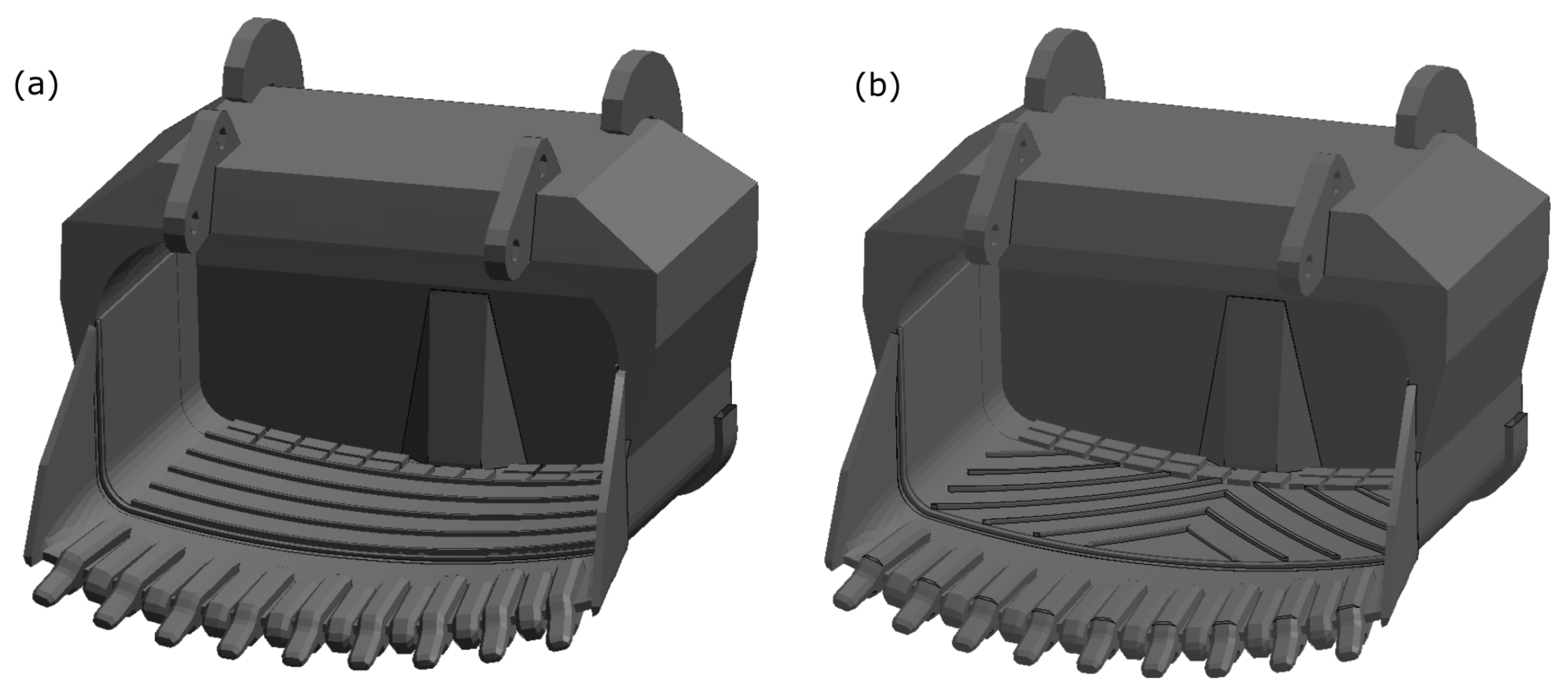
The validated model was used to evaluate how different geometrical changes in, e.g., a rope shovel bucket affects wear, dig force, and filling degree. Two examples of utilizing the model were investigated in order to evaluate if the present model was suitable for such a task. The approach was to perform simulations when changes were made to the bucket and further evaluate the changes in wear, dig force, and bucket filling degree. Comparisons between the original bucket used for the validation case and the two buckets with added features were performed. The buckets with added features in the form of steel bars at 90° and 45° angles to the direction of the material flow are shown in Figure 10. The material of the steel bars were the same as for the remaining bucket. The only difference between the new and the baseline model setup was the added steel bars. Ten bucket filling cycles were repeated for all the comparisons.
4. Results and Discussion
In this section, the result from the wear simulations will be presented. The validity of the rope shovel and granular material model is not presented here. In previous work by Svanberg et al. [38], it was demonstrated that the developed numerical model excellently captures the full-scale phenomenon of the granular material and the contact mechanics with a structural component such as a bucket. Validation of the model with experimental full-scale observed data shows strong agreement.
4.1. Wear Model Calibration
The calibration of the wear model was performed by determining suitable parameters and values of mesh size on structure components, the particle size distribution of granular material and smoothing cycles. The choices were based on the result from the sensitivity analysis, also keeping in mind the intent to perform full-scale simulations with realistic computational time. Hence, for the calibration of the model, a mesh size of 75 mm was chosen as a suitable mesh size concerning particle size distribution and resolution of geometry. The ratio between the baseline granular material model with the smallest particle of a radius, R = 100 mm and the element size is RI = 1.33. The amount of smoothing iterations was set to one for all simulations. Since smoothing is artificially applied to the wear depth, the iterations were kept as low as possible, however, still receiving the benefits of using the weighted average smoothing function. The baseline granular material model is the same as presented in previous work [38]. The smallest particle has a radius of 100 mm. However, to see the effect of including smaller particles, another granular material model was generated containing particles with the smallest particle diameter of R = 50 mm.
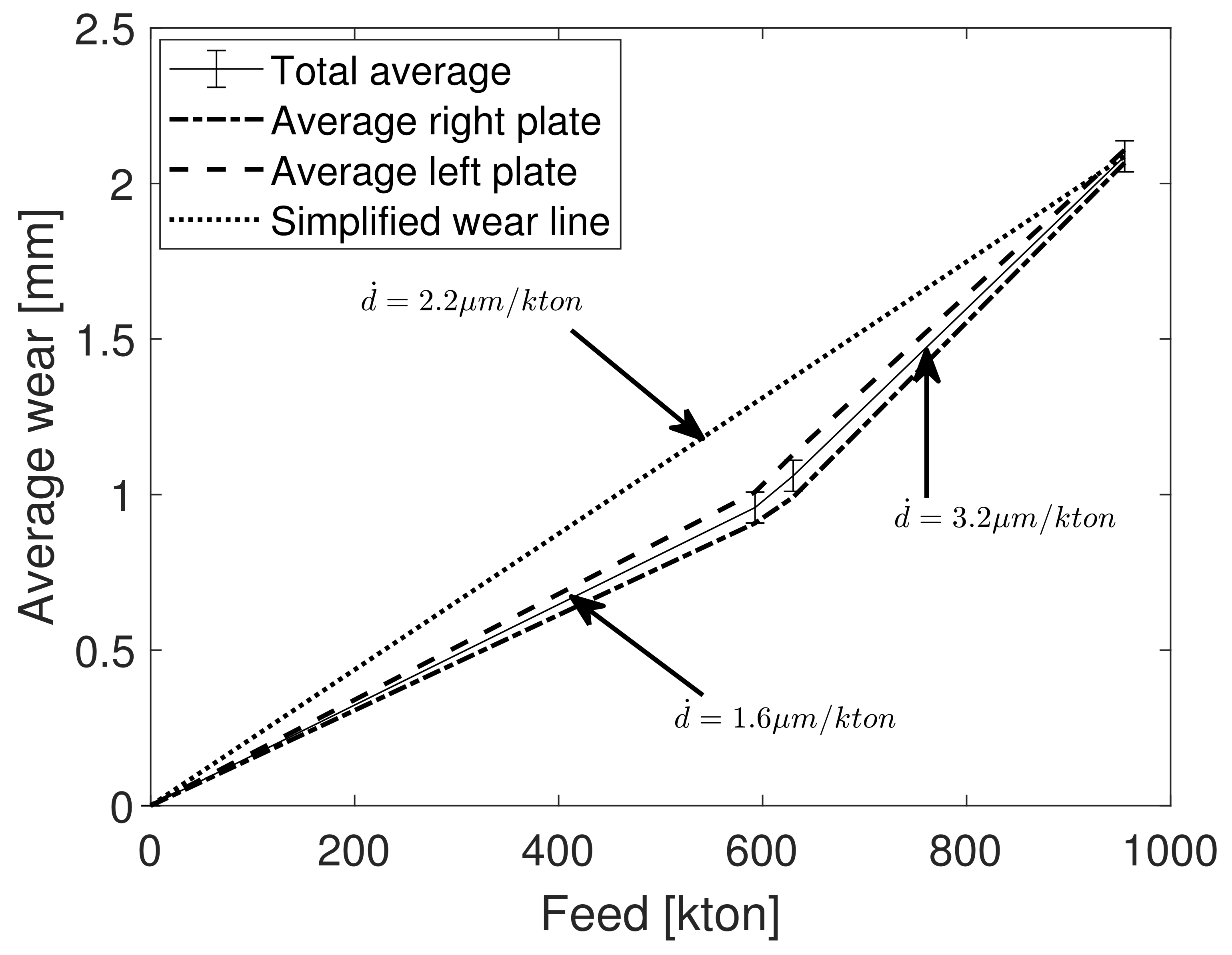
In Figure 11, the experimental results from the wear measurement on the plates belonging to the vibratory feeder are shown. A total of three measuring occasions were performed, giving approximately two linear wear gradients/rates (wear depth/tonnage). A simplified wear rate was used for calibrating the wear model. The simplified wear rate is the line with = 2.2 µm/kton in Figure 11.
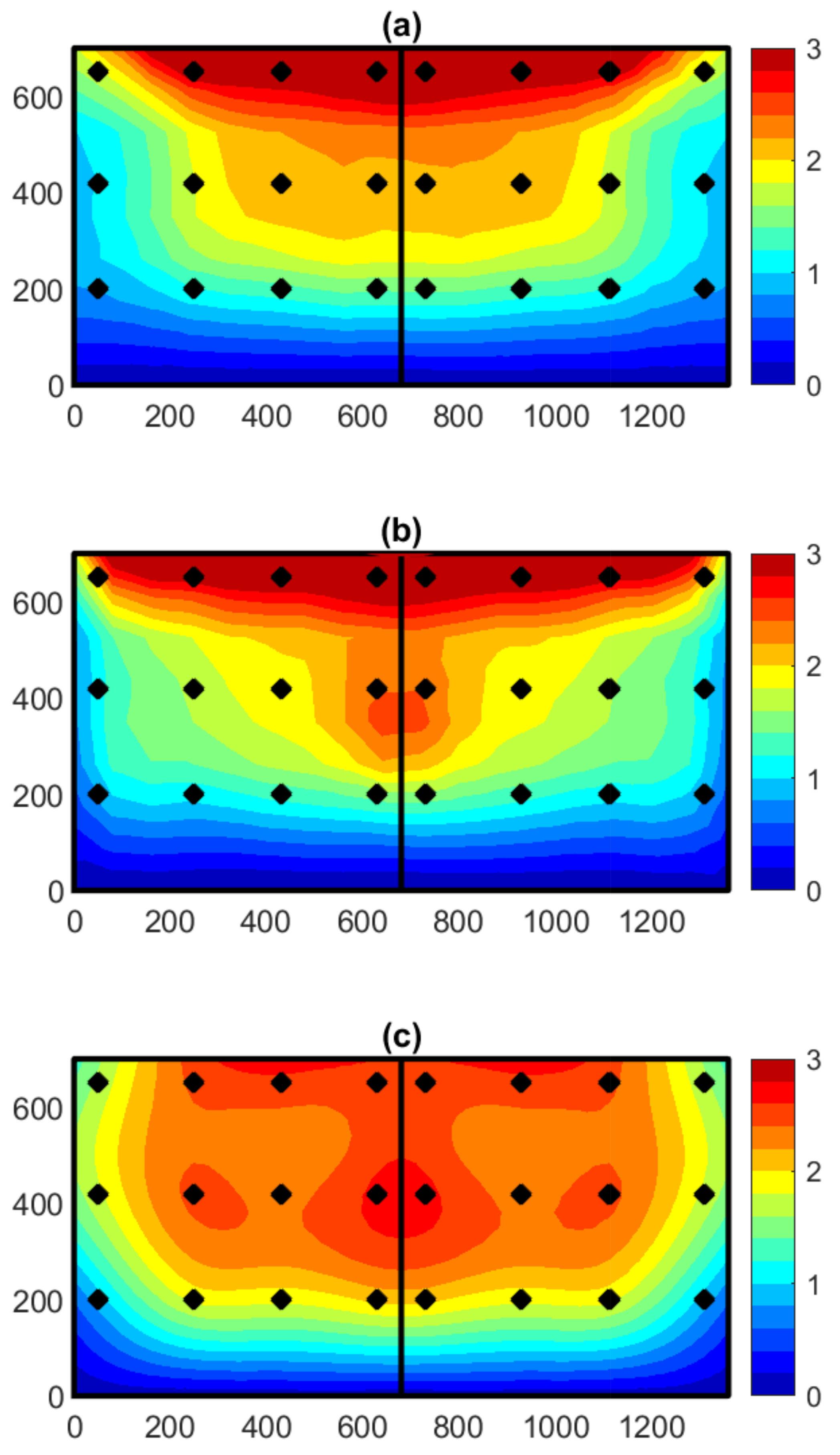
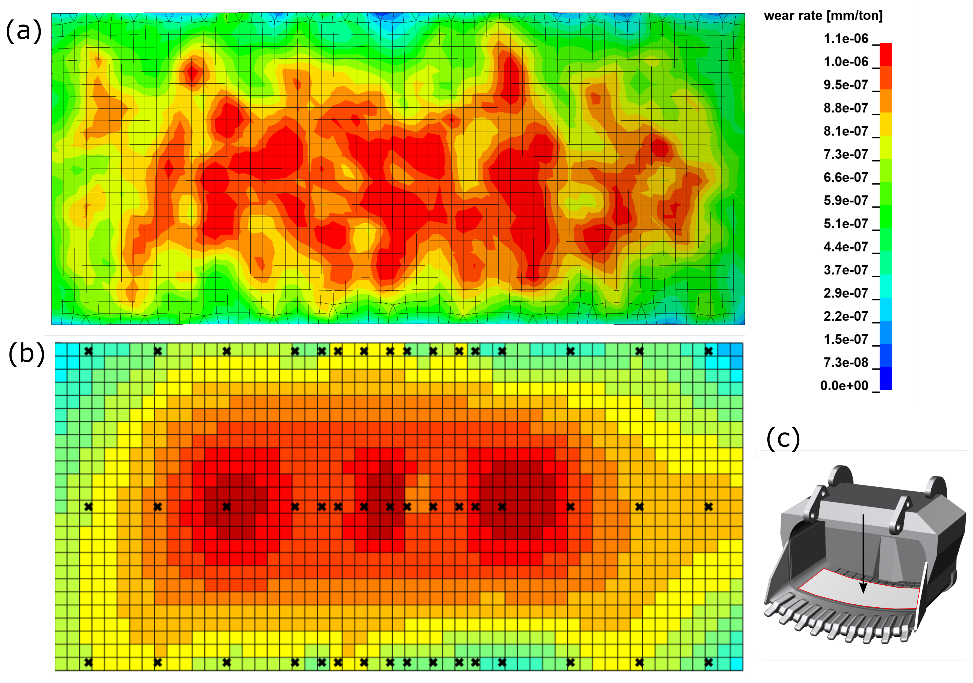
The results from the calibration are presented in Figure 12. Simulated absolute wear maps from the two bottom plates are shown in Figure 12a,b for the two cases where smaller and larges particles are used. A total of approximately 45 tonnes of material was going through the feeder in the simulations. This is to be compared to approximately 955 ktonnes for the experiments. The experimental wear map is solely based on the black dots seen in Figure 12c, whereas the simulated wear maps are the actual wear map from simulations. However, both for the experimental and simulated wear maps, the average of the left and right sides are taken, and further mirrored in order to obtain more comparable absolute wear maps. The average wear from the simulations is the same as the experimental wear after calibration. This proves that the calibration is sufficiently performed. Comparing the wear maps between simulation and experimental results (Figure 12), it is clear that the general trend is captured in the simulations for both the case of R = 50 and R = 100 mm. However, the experimental wear seems to be somewhat more even. The locations of most wear for all three cases occur in the center where the two plates meet, and to the front of the plates.
4.2. Sensitivity Analysis
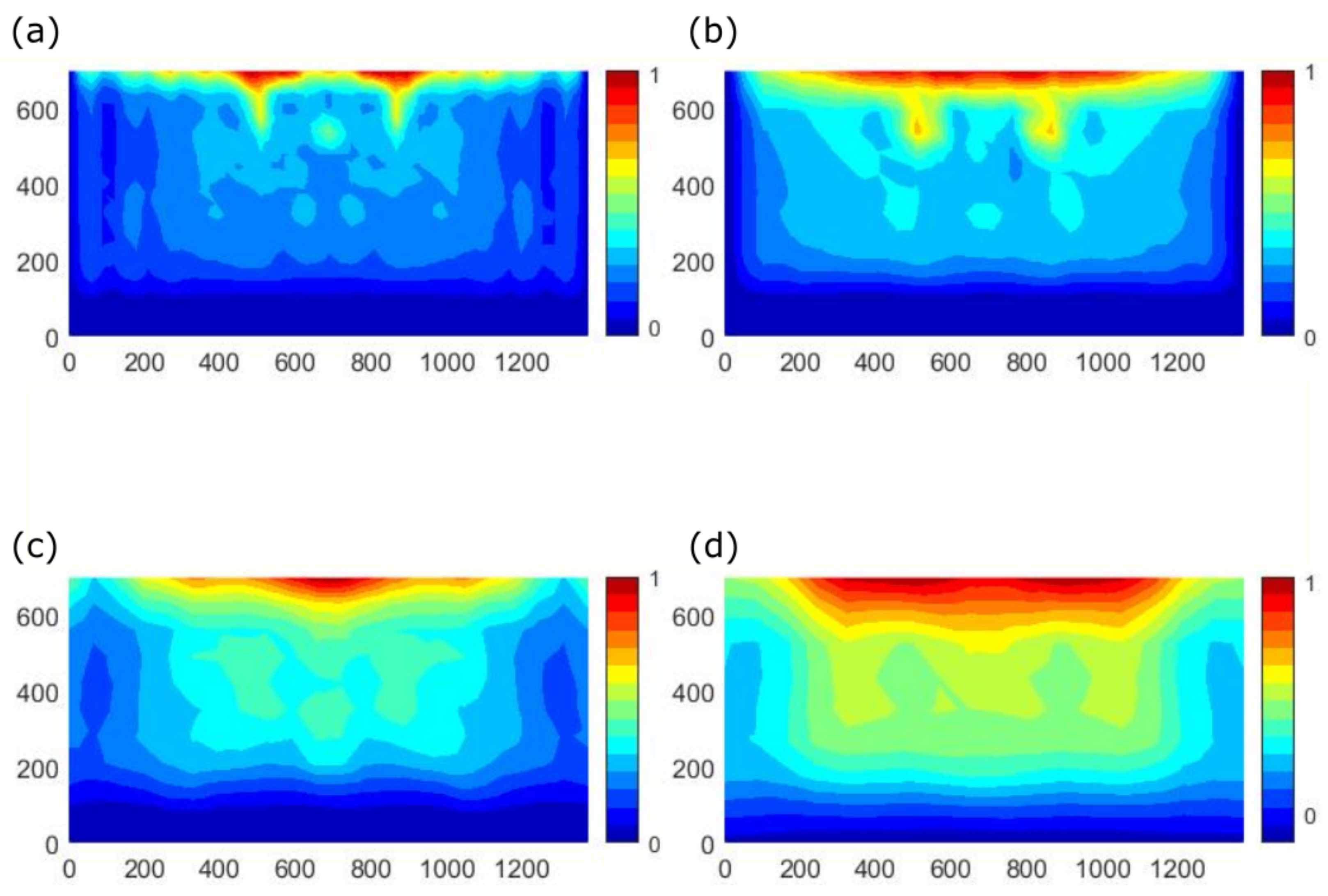
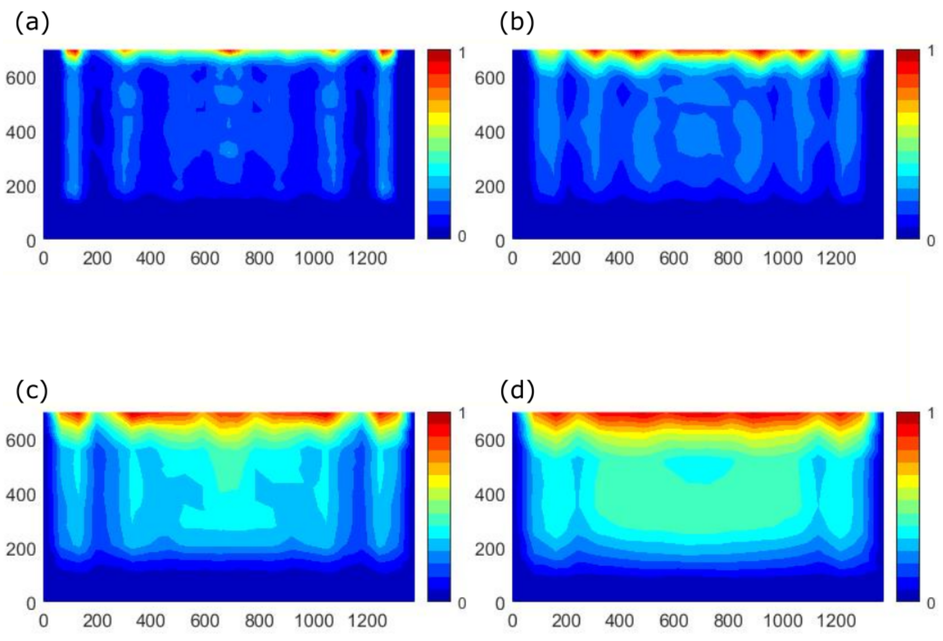
The two different particle sizes and the four mesh sizes were investigated by performing simulations and evaluating the wear results. In Figure 13 and Figure 14, results from varying the mesh size when using the smaller and the larger particle are shown. Results in Figure 13 and Figure 14 are normalized and mirror averaged. From the results, it is clear that the wear distribution over the plates varies with mesh size. However, when comparing the different particle sizes, the wear distribution seems to be changing similarly. In Figure 14, where the coarser PSD was used, on the far left and far right sides of the wear plates, localization of wear in form of lines is observed. This is because the larger particles cannot reach the corners. For the smaller particles, this behavior is not observed since the particles are smaller. The contact between, e.g., a DE sphere and a surface is defined through the contact area. Due to the penalty-based contact law and because the relatively small penetrations, the theoretical contact area also becomes small and, i.e., never exceeds the size of one element. This means that contact occurs only for one element for the same time step. Hence, the behavior presented when changing particle size can be explained. In other words, if a 10 mm sphere or a 100 mm sphere would hit a surface defined with elements, there would only be one element with any calculated wear.
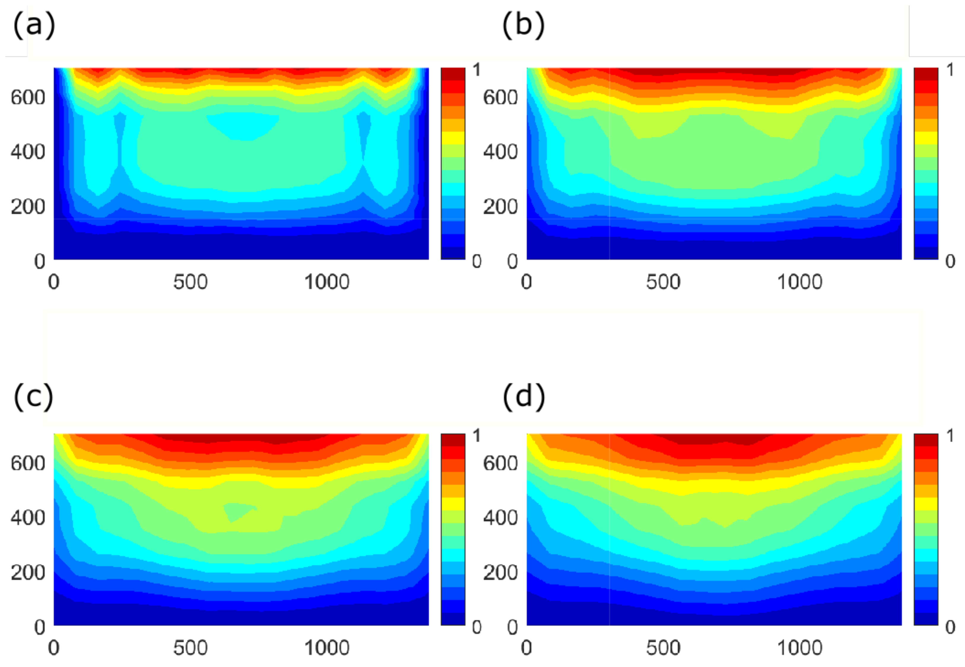
The influence of different amounts of smoothing is presented in Figure 15. The smoothing kernel is applied on a wear map from the calibration simulation. As can be observed from Figure 15a–d, the smoothing effect has the largest influence between no smoothing and one smoothing iteration for the present mesh size and particle size distribution of the granular material.
4.3. Model Validation
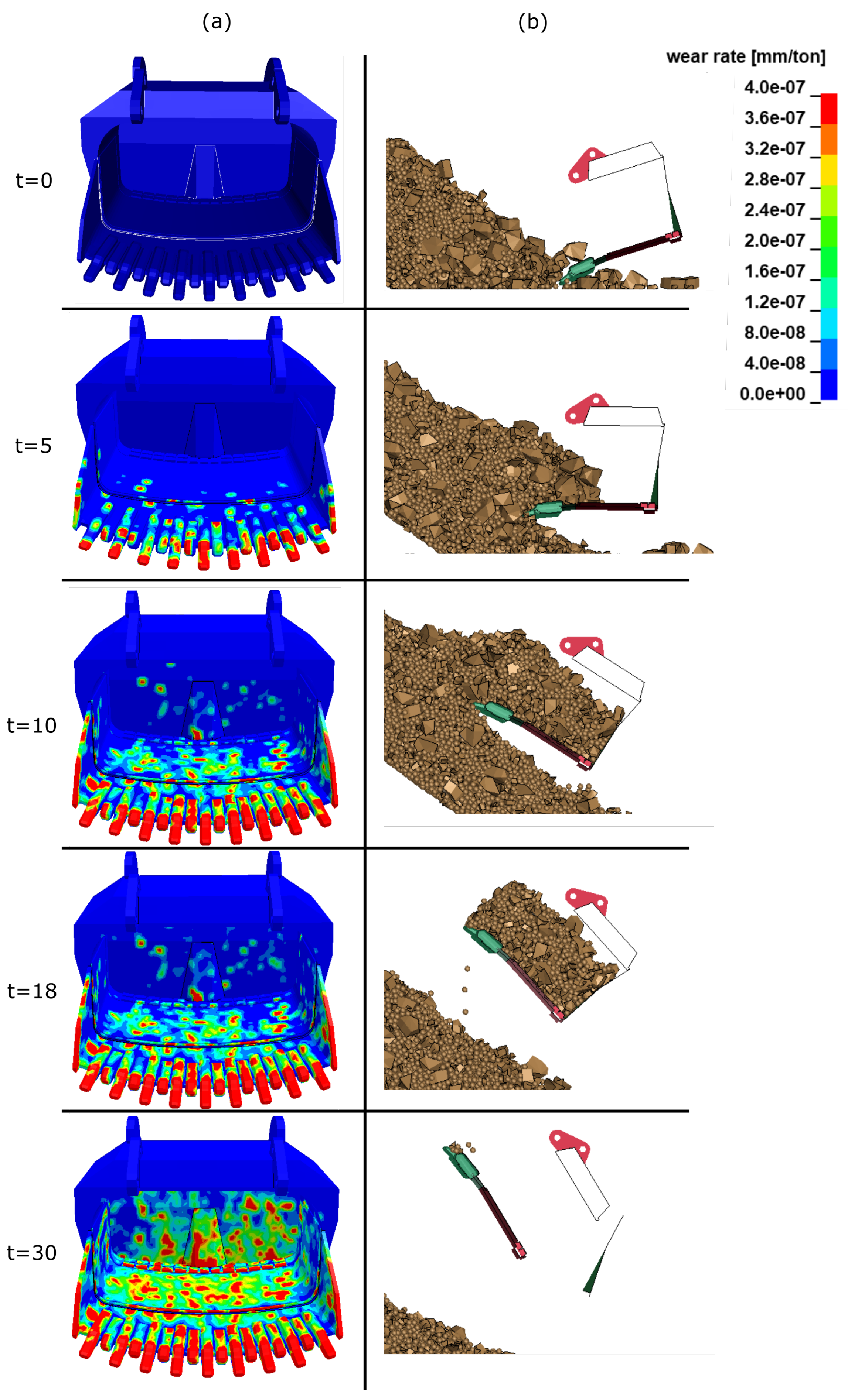
Validation of the wear simulation model was performed by comparing the experimental wear measurements described in Section 2.2 with the predicted wear from the simulations. The wear results from a total of 28 bucket fillings with varying masses were added together and smoothed once. The total loaded mass from the simulations was 1631 tonnes. The mass in the real bucket between the experimental wear measurements was 3583 kton. To facilitate a comparison between experimental and simulated wears, the total wear was divided with actual tonnage, giving a wear rate in (mm/ton) that is versatile for comparison. In Figure 16, snapshots from the wear simulation are shown at different stages during one bucket filling. From the snapshots, it is clear that the wear contribution during the first five seconds is located in the front of the bucket and the lip. During emptying of the bucket, the majority of the wear from the back and on the door is dominating. In Figure 17, a 3D overview of the wear on the bucket is shown.
In Figure 18, a comparison between simulated and experimental wear depth of the bottom plates is shown. The comparison highlights that the predicted wear from the simulation is giving wear concentrations at approximately the same positions as the experiments and that the level of wear is agreeing properly with the experimental results. The wear from the experiments are considerably more smooth and more uniform than the simulated results. The reason for this behavior, could be the large difference between the actual cycles and the simulated amount of cycles. Since there are approximately 1500 times more real cycles than simulated, it is obvious that the model cannot capture all possible scenarios of particle–structure interaction that cause wear. Another cause is that the present model does not contain the finer particles of the PSD.
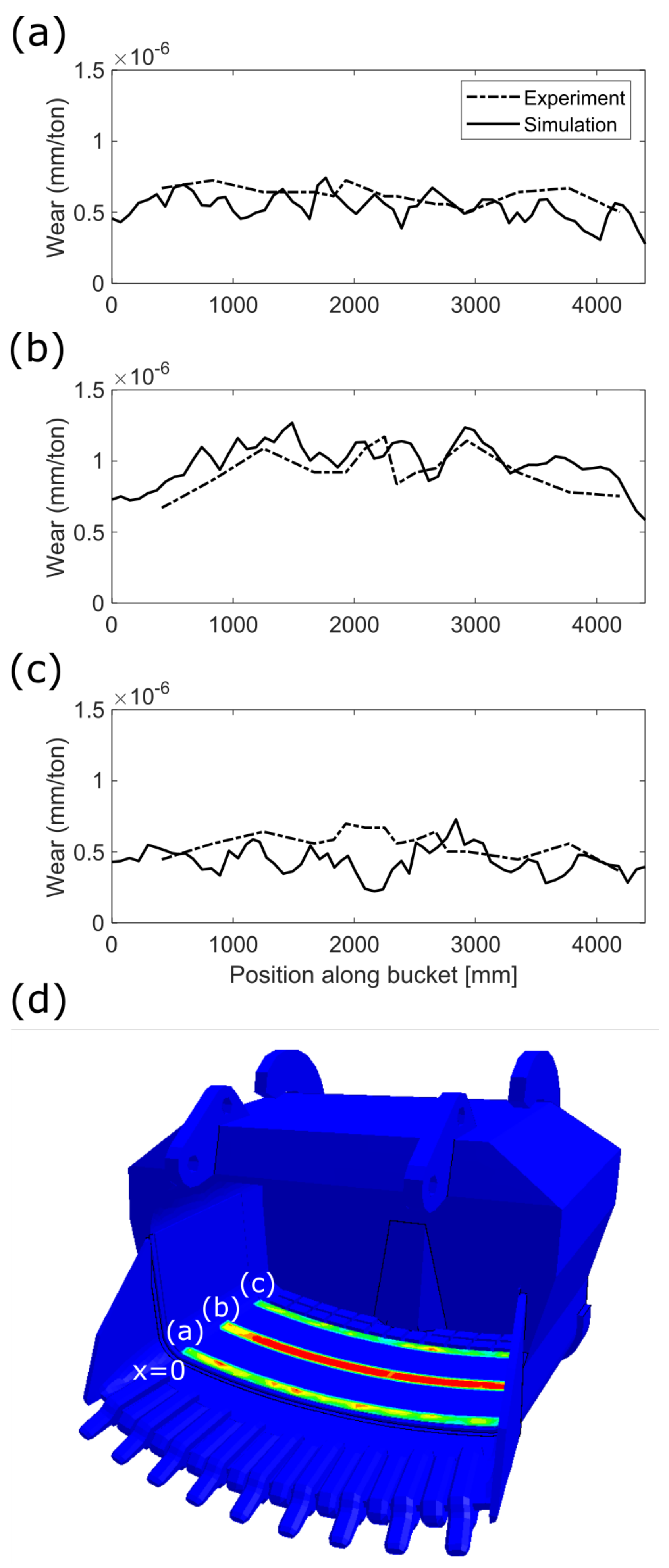
To compare the wear more quantitatively, the wear was plotted along sections of the bucket, which is presented in Figure 19. The simulated wear along the three sections correlates very well to the experimental results. Both the absolute value of the wear and the trends along the width are in agreement.
The simulated wear results were further compared to other experimental measurements on the inner side plates on both left and right sides, as well as the bucket door. The conclusion from the comparison is that the general wear behavior is captured. Both the magnitude of the wear rate, as well as the wear map, are captured. However, the experimental results show a smoother result than the predictions from simulations. The reason for this discrepancy is likely the larger number of bucket filling cycles in combination with the finer particles present in reality as previously mentioned.
4.4. Application of Model to Minimize Wear
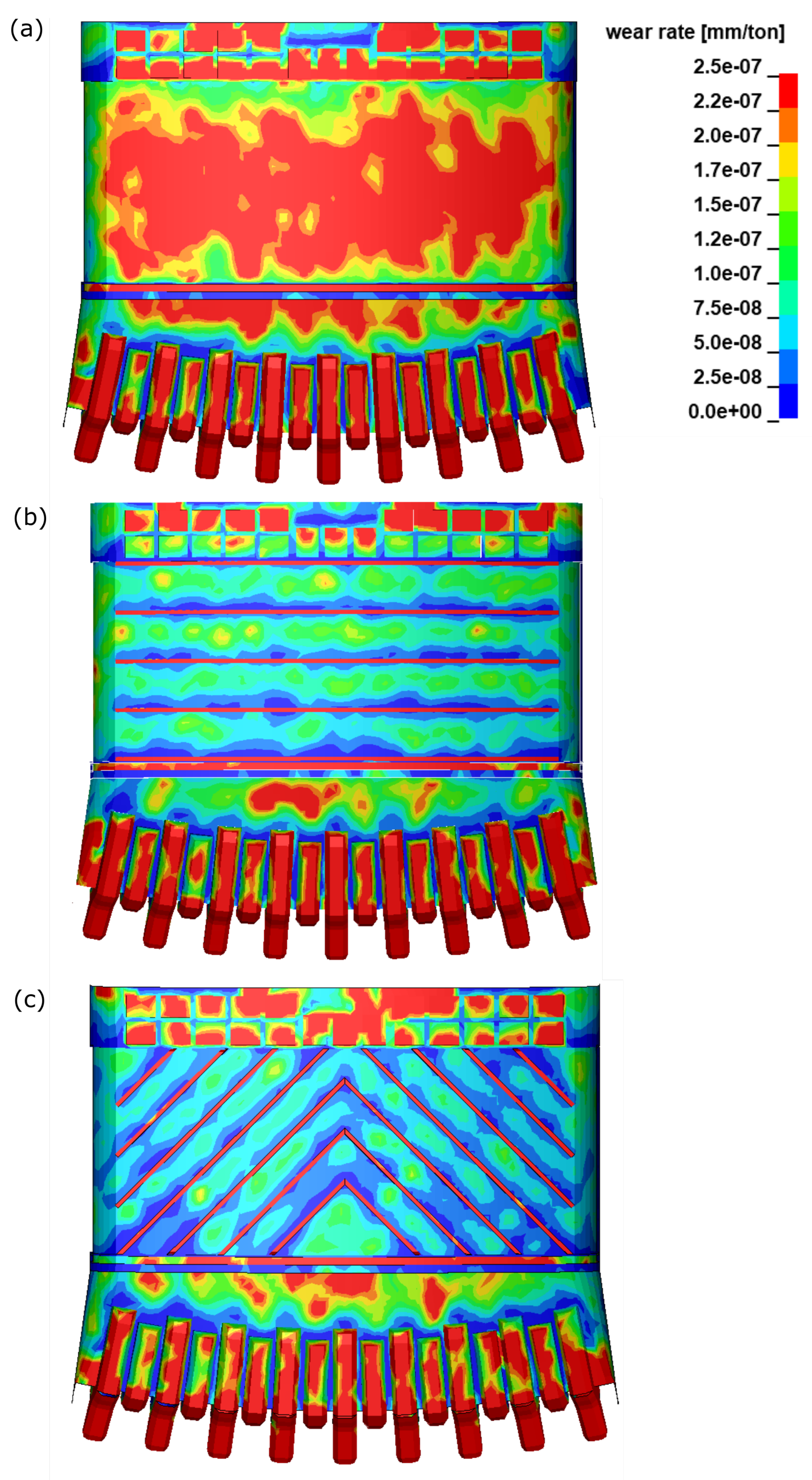
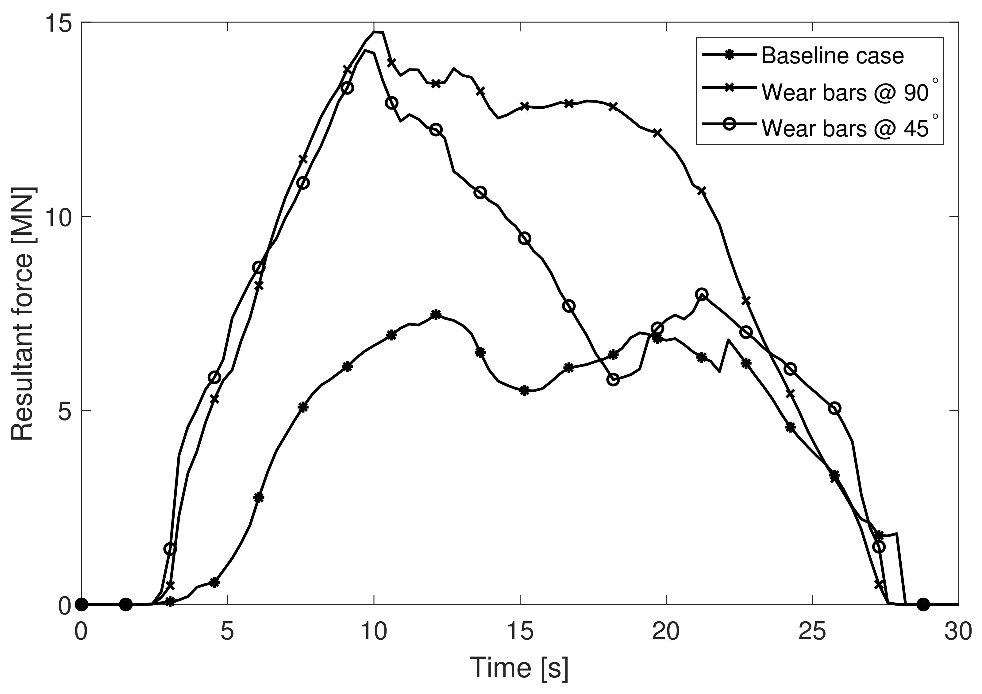
In Figure 20, the wear maps from the baseline bucket, and the new buckets are compared. The wear from the new bucket on the bottom plates is reduced by approximately 2–5 times compared to the baseline bucket. For the case when the steel bars are at 90°, the wear on the large blocks in the rear and close to the hatch are also greatly reduced for the new geometry. For both cases when wear bars are used, the larger portion of wear is absorbed by the steel bars. Hence, the wear has been moved to a position where the maintenance downtime will be highly reduced compared to replacing the bottom plates. By only looking at the wear rate maps, it is clear that by simply adding the steel bars, the wear on the bottom plates is significantly reduced, and the service life of the bottom plates could be extended with several times compared to the current service life. This, of course, demands that the steel bars are replaced when worn down. However, there are other aspects to the bucket geometry. For example, the diggability and filling degree. In Figure 21, the resultant interface forces between the buckets and granular material are plotted for the baseline bucket and the new buckets with the steel bars. It is clear that the added steel bars significantly increase the digging force. In this way, the diggability significantly gets worse since it is more resistant when penetrating the material. The steel bars located at 90° give the largest average dig force, and for the 45° bars, a smaller average force is observed. However, the peak forces are approximately the same. When comparing the bucket filling degree for the three different cases, no difference was observed between the baseline case and when the bars were located at 45°, however, for the case with wear bars at 90°, a decrease of approximately 3% was observed. The results presented in Figure 20 and Figure 21 are in agreement with what has been observed in the Aitik mine. Hence, these examples of changing the bucket geometry demonstrates that the present model can capture the influences of wear and at the same time detect how the dig force and bucket filling degree are affected.
4.5. General Discussion
In this paper, a numerical model for simulating wear at full-scale in a harsh sub-arctic environment is presented and validated, and the use of the model is demonstrated with two examples. The wear simulator employs a unique numerical model previously presented [38]. An in-house wear model is developed and coupled to the simulation environment. Furthermore, the wear model is calibrated in a full-scale in situ environment, and then the wear model is applied to the loading process. Validation of the wear model is performed at full-scale with experimental wear measurements on a rope shovel bucket.
From the results presented in Section 4.1, it is clear that the one-step calibration process is simplified compared to reality. By looking at the experimentally average wear rate in Figure 11, it is obvious that the wear rate changes with the feed of material. The reason is that the experimental wear is non-linear, and this can depend on various reasons. One of the reasons could be that the crusher is a mobile equipment with the possibility to move, hence, the type of material going through the feeder changes. During the second, third, and fourth measurements, the feeder changed location in the mine and the operators of the crusher recognized an increased hardness of the material, which partly could explain the increased wear rate after the second measurement. It is also known that the wear rate in general is non-linear [41]. The reason for the non-linear wear rate could be because of the change of material flow when the geometry is changed due to wear. This is sometimes refereed to as accelerated wear, when wear is accelerating wear. Another explanation is that the hardness of the wear plates is not constant through the thickness, and it also changes from, e.g., work hardening and temperature conditions. Most likely, the phenomenon is dependent on the two mentioned explanations. To include all these effects in the model, it requires a more advanced model than presented herein. To address the mentioned problems related to the calibration process would be a significant improvement of the present work; however, it is out of scope for this study.
The wear model, presented in Section 3.2, was developed with the aim to be an easily calibrated wear model for industrial full-scale predictions when both sliding and impact wear are present. The limitations of the commonly used Finnie’s wear model were identified and further modified to better suit applications when sliding and impact wear are present. It should be mentioned that the model was investigated for several different impact angles ranging from zero to 90°, and the model showed a clear dependency on the impact angle, though the angle-terms were neglected in the original Finnie model. The aim of the wear model is to obtain a model that can deal with sliding and impact wear and be suitable for full-scale industrial use. The purpose was to calibrate and validate the model in similar environments as it was supposed to be used for, and not use a perfect lab-scale environment with high resolution measurements. Since both the calibration and validation show a good agreement of the relative wear maps, it can be assumed that the model is capturing the main phenomenons of how wear proceeds for these type of applications.
From the result presented from the mesh and particle size sensitivity analysis in Section 4.2, it was shown that the wear depth was dependent on the mesh and particle sizes in the model. For computational cost savings, a cut-off value of the smallest particles in the granular model with R = 100 mm was introduced. This resulted in that all local effects related to wear from the fines are not captured in the model. However, since the computational cost rapidly increases with smaller particles, it was not assumed adequate to reduce the particle size. The increase in computational time is partly due to the smaller explicit time step required for a stable solution and partly because of the increase in particle count, which in turn causes more contacts. However, a more thorough study of the particle size influence would be of great interest.
In the present work, the bucket filling process was simulated by repeating the same bucket trajectory for three different piles. In reality, a variety of the trajectory is observed depending on the loading situation, the skill of the operators, etc. Furthermore, the simulated amount of cycles is 1500 times lower than in reality. Yet, the model has proven that the result from a few cycles can give very useful and interesting results that agree well with experiments. When making assumptions and simplifications, it is of great importance to be aware of important variables within each process, and make case-specific decisions based on the present application.
From the validation of the model, it was demonstrated that the wear model is suitable for full-scale applications where both sliding and impact wear occur, see Section 4.3. The simulated wear maps and magnitude of wear related to the bottom plates, door, plates on the inside and outside shows a good agreement when compared to the experiments. Furthermore, simulated wear maps from the lip and teeth are in agreement; however, the magnitude of wear is not sufficiently good. The reason for this is most likely that the lip material is cast steel, which is different from the wear plate material against which the calibration was performed. As mentioned in Section 2, there is a difference between the steel plates in calibration and the rope shovel bucket steel plates. For the rope shovel, Hardox 500 is used, and for the calibration, Hardox 450 is used. The reason for this is that the study was limited to in situ testing, and the authors argued that the Hardox 450 would serve as a relevant base for calibration. As previously mentioned, perhaps the full-scale calibration is more important than having the exact same material, despite not being at full-scale. Once again, a balancing was made between the full-scale approach and the exactness of the test.
When the geometry was changed by including the steel bars, a clear reduction of the wear was observed, see Figure 20; however, at the cost of an increased dig force due to increased resistance between bucket and particles, see Figure 21. No significant change in bucket filling degree for most of the cases was observed. The result from the comparison shows that it is adequate to assume that the model can be used as a tool for making better decisions related to wear and diggability. A balancing between dig force and wear is of utmost importance to ensure that both the production and the maintenance crew are satisfied.
In this paper, the work has focused on electric rope shovels during the loading process; however, the experimental and numerical methods are not limited to these applications. Since the presented methods are fairly versatile methods suitable for numerous applications where granular materials are occurring, the methods developed in this work can be fairly comfortably transferred to other applications. If the model is utilized correctly, it can lead to a significant reduction of wear, and increase the service life of components.
5. Conclusions
This work covers numerical modeling, calibration, simulation and validation of wear development in an electric rope shovel at full-scale. The in-house wear model is developed and coupled to the simulation environment and applied to the loading process. The major conclusions from the methods and results in this paper are presented in this section.
- An in-house wear model that considers both abrasive sliding and impact wear is developed.
- The granular material model in combination with the presented wear model shows that the major phenomenon of wear is captured by the model.
- Full-scale validation for a rope shovel bucket proves that the simulated wear is agreeing well with experimentally measured wear.
- By changing the geometry of the bucket, it shows that the wear is significantly reduced. However, on the cost of increased dig force. This concludes that the model is suitable to use as a tool for optimizing wear.
- Full-scale in situ calibration and validation experiments are presented.
- The numerical and experimental methods presented increases the knowledge of wear phenomenon for full-scale and large processes.
- The presented simulation model is suitable for product development and optimization of the loading process.
Author Contributions
Conceptualization, A.S., S.L., R.M. and P.J.; methodology, A.S., S.L., R.M. and P.J.; software, A.S.; validation, A.S., S.L., R.M. and P.J.; formal analysis, A.S., S.L., R.M. and P.J.; investigation, A.S., S.L., R.M. and P.J.; resources, A.S., S.L., R.M. and P.J.; writing—original draft preparation, A.S. and S.L.; writing—review and editing, A.S., S.L., R.M. and P.J.; visualization, A.S.; supervision, S.L., R.M. and P.J.; project administration, P.J. and R.M.; funding acquisition, P.J. All authors have read and agreed to the published version of the manuscript.
Funding
This research was funded by KIC RawMaterials through the project “HARSHWORK”, Project Agreement No. 17152.
Institutional Review Board Statement
Not applicable.
Informed Consent Statement
Not applicable.
Data Availability Statement
Not applicable.
Acknowledgments
For financial support of the Project “HARSHWORK”, Project Agreement No. 17152, KIC RawMaterials is gratefully acknowledged. The authors wish to thank personnel at Boliden for useful insights and help during this work. Daniel Oderstål at Bottnia Kross AB is acknowledged for help regarding the calibration experiment.
Conflicts of Interest
The authors declare no conflict of interest. The funders had no role in the design of the study; in the collection, analyses, or interpretation of data; in the writing of the manuscript, or in the decision to publish the results.
References
- Holmberg, K.; Erdemir, A. Influence of tribology on global energy consumption, costs and emissions. Friction 2017, 5, 263–284. [Google Scholar] [CrossRef]
- Bayer, R.G. Fundamentals of Wear Failures. In Failure Analysis and Prevention; ASM International: Novelty, OH, USA, 2002. [Google Scholar] [CrossRef]
- Kato, K.; Adachi, K. Modern Tribology Handbook; CRC Press: Boca Raton, FL, USA, 2001; Volume 1, pp. 273–300. [Google Scholar]
- Straffelini, G. Friction and Wear: Methodologies for Design and Control; Springer: Cham, Switzerland, 2015. [Google Scholar] [CrossRef]
- Archard, J.F. Contact and rubbing of flat surfaces. J. Appl. Phys. 1953, 24, 981–988. [Google Scholar] [CrossRef]
- Rabinowicz, E. The Effect of Size on the Looseness of Wear Fragments. Wear 1958, 2, 4–8. [Google Scholar] [CrossRef]
- Popova, E.; Popov, V.L.; Kim, D.E. 60 years of Rabinowicz’ criterion for adhesive wear. Friction 2018, 6, 341–348. [Google Scholar] [CrossRef]
- Finnie, I. Erosion of Surfaces By Solid Particles. Wear 1960, 3, 87–103. [Google Scholar] [CrossRef]
- Magnée, A. Generalized Law of Erosion: Application to Various Alloys and Intermetallics. Wear 1995, 181–183, 500–510. [Google Scholar] [CrossRef]
- Bitter, J.G.A. A Study of Erosion Phenomena: Part I. Wear 1963, 6, 5–21. [Google Scholar] [CrossRef]
- Rizkalla, P.; Fletcher, D.F. Development of a slurry abrasion model using an Eulerian–Eulerian ‘two-fluid’ approach. Appl. Math. Model. 2017, 44, 107–123. [Google Scholar] [CrossRef]
- Zhao, Y.; Ma, H.; Xu, L.; Zheng, J. An erosion model for the discrete element method. Particuology 2017, 34, 81–88. [Google Scholar] [CrossRef]
- Ashrafizadeh, H.; Ashrafizadeh, F. A numerical 3D simulation for prediction of wear caused by solid particle impact. Wear 2012, 276–277, 75–84. [Google Scholar] [CrossRef]
- Cundall, P. A computer model for simulating progressive large scale movements in blocky rock systems. In Proceedings of the International Symposium on Rock Mechanics, Nancy, France, 4–6 October 1971; pp. 2–8. [Google Scholar]
- Cundall, P.A.; Strack, O.D.L. A discrete numerical model for granular assemblies. Géotechnique 1979, 29, 47–65. [Google Scholar] [CrossRef]
- Kelly, C.; Olsen, N.; Negrut, D. Billion degree of freedom granular dynamics simulation on commodity hardware via heterogeneous data-type representation. Multibody Syst. Dyn. 2020, 50, 355–379. [Google Scholar] [CrossRef]
- Gan, J.; Evans, T.; Yu, A. Application of GPU-DEM simulation on large-scale granular handling and processing in ironmaking related industries. Powder Technol. 2020, 361, 258–273. [Google Scholar] [CrossRef]
- Cleary, P.W. Effect of rock shape representation in DEM on flow and energy utilisation in a pilot SAG mill. Comput. Part. Mech. 2019, 6, 461–477. [Google Scholar] [CrossRef]
- Larsson, S.; Prieto, J.M.R.; Heiskari, H.; Jonsén, P. A novel particle-based approach for modeling a wet vertical stirred media mill. Minerals 2021, 11, 55. [Google Scholar] [CrossRef]
- Jonsén, P.; Hammarberg, S.; Pålsson, B.I.; Lindkvist, G. Preliminary validation of a new way to model physical interactions between pulp, charge and mill structure in tumbling mills. Miner. Eng. 2019, 130, 76–84. [Google Scholar] [CrossRef]
- Quist, J.; Evertsson, C.M. Cone crusher modelling and simulation using DEM. Miner. Eng. 2016, 85, 92–105. [Google Scholar] [CrossRef]
- Roessler, T.; Katterfeld, A. Development of a Standardized Procedure for the Calibration of DEM Abrasive Wear Simulations; White Paper-Calibration of DEM Parameters for Cohesionless Bulk Materials under Rapid Flow Conditions and Low Consolidation View Project Research on the Application of the Discrete Element Method in Bulk Material Handling View Project. In Proceedings of the CHoPS 2018—9th International Conference on Conveying and Handling of Particulate Solids, Technical Report. London, UK, 10–14 September 2018. [Google Scholar]
- Ilic, D. Development of design criteria for reducing wear in iron ore transfer chutes. Wear 2019, 434–435, 202986. [Google Scholar] [CrossRef]
- Perazzo, F.; Löhner, R.; Labbe, F.; Knop, F.; Mascaró, P. Numerical modeling of the pattern and wear rate on a structural steel plate using DEM. Miner. Eng. 2019, 137, 290–302. [Google Scholar] [CrossRef]
- Quist, J.; Franke, J.; Evertsson, M. The Effect of Liner Wear on Gyratory Crushing: A DEM Case Study. In Proceedings of the 3rd International Computational Modelling Symposium by MEI, Langkawi, Malaysia, 20–22 September 2011. [Google Scholar]
- Larsson, S.; Pålsson, B.I.; Parian, M.; Jonsén, P. A novel approach for modelling of physical interactions between slurry, grinding media and mill structure in wet stirred media mills. Miner. Eng. 2020, 148, 106180. [Google Scholar] [CrossRef]
- Xu, L.; Luo, K.; Zhao, Y. Numerical prediction of wear in SAG mills based on DEM simulations. Powder Technol. 2018, 329, 353–363. [Google Scholar] [CrossRef]
- Cleary, P.W.; Owen, P.; Hoyer, D.I.; Marshall, S. Prediction of mill liner shape evolution and changing operational performance during the liner life cycle: Case study of a Hicom mill. Int. J. Numer. Methods Eng. 2010, 81, 1157–1179. [Google Scholar] [CrossRef]
- Boemer, D. Discrete Element Method Modeling of Ball Mills-Liner Wear Evolution. Ph.D. Thesis, University of Liège, Liège, Belgium, 2014. [Google Scholar]
- Kalala, J.T. Discrete Element Method Modelling of Forces and Wear on Mill Lifters in Dry Ball Milling. Ph.D. Thesis, University of the Witwatersrand, Johannesburg, South Africa, 2008. [Google Scholar]
- Zhao, L.; Jin, X.; Liu, X. Numerical research on wear characteristics of drum based on discrete element method (DEM). Eng. Fail. Anal. 2020, 109. [Google Scholar] [CrossRef]
- Jafari, A.; Saljooghi Nezhad, V. Employing DEM to study the impact of different parameters on the screening efficiency and mesh wear. Powder Technol. 2016, 297, 126–143. [Google Scholar] [CrossRef]
- Jafari, A.; Abbasi Hattani, R. Investigation of parameters influencing erosive wear using DEM. Friction 2020, 8, 136–150. [Google Scholar] [CrossRef] [Green Version]
- Rojas, E.; Vergara, V.; Soto, R. Case study: Discrete element modeling of wear in mining hoppers. Wear 2019, 430–431, 120–125. [Google Scholar] [CrossRef]
- Forsström, D.; Jonsén, P. Calibration and validation of a large scale abrasive wear model by coupling DEM-FEM: Local failure prediction from abrasive wear of tipper bodies during unloading of granular material. Eng. Fail. Anal. 2016, 66, 274–383. [Google Scholar] [CrossRef]
- Forsström, D.; Lindbäck, T.; Jonsén, P. Prediction of wear in dumper truck body by coupling SPH-FEM. Tribol. Mater. Surf. Interfaces 2014, 8, 111–115. [Google Scholar] [CrossRef]
- Nyberg, U.; Esen, S.; Bergman, P.; Ouchterlony, F. Uppföljning av Styckefallet i Salva 4141-2 i Aitikgruvan; Technical Report; Luleå University of Technology: Luleå, Sweden, 2006. [Google Scholar]
- Svanberg, A.; Larsson, S.; Mäki, R.; Jonsén, P. Full-scale simulation and validation of bucket filling for a mining rope shovel by using a combined rigid FE-DEM granular material model. Comput. Part. Mech. 2020. [Google Scholar] [CrossRef]
- LSTC. LS-DYNA Theory Manual; Livermore Software Technology Corporation: Livermore, CA, USA, 2019. [Google Scholar]
- Borrvall, T.; Jernberg, A.; Schill, M.; Deng, L.; Oldenburg, M. Simulation of Wear Processes in LS-DYNA. In Proceedings of the 14th International LS-DYNA Users Conference Simulation of Wear Processes in LS-DYNA®, Technical Report. Dearborn, MI, USA, 12–14 June 2016. [Google Scholar]
- Yang, L.J. A methodology for the prediction of standard steady-state wear coefficient in an aluminium-based matrix composite reinforced with alumina particles. J. Mater. Process. Technol. 2005, 162–163, 139–148. [Google Scholar] [CrossRef]
Figure 1.
Particle size distribution (PSD) used as a base for the granular material model. PSD curve from one blasting in the Aitik mine. The curve is adopted from [37].
Figure 1.
Particle size distribution (PSD) used as a base for the granular material model. PSD curve from one blasting in the Aitik mine. The curve is adopted from [37].

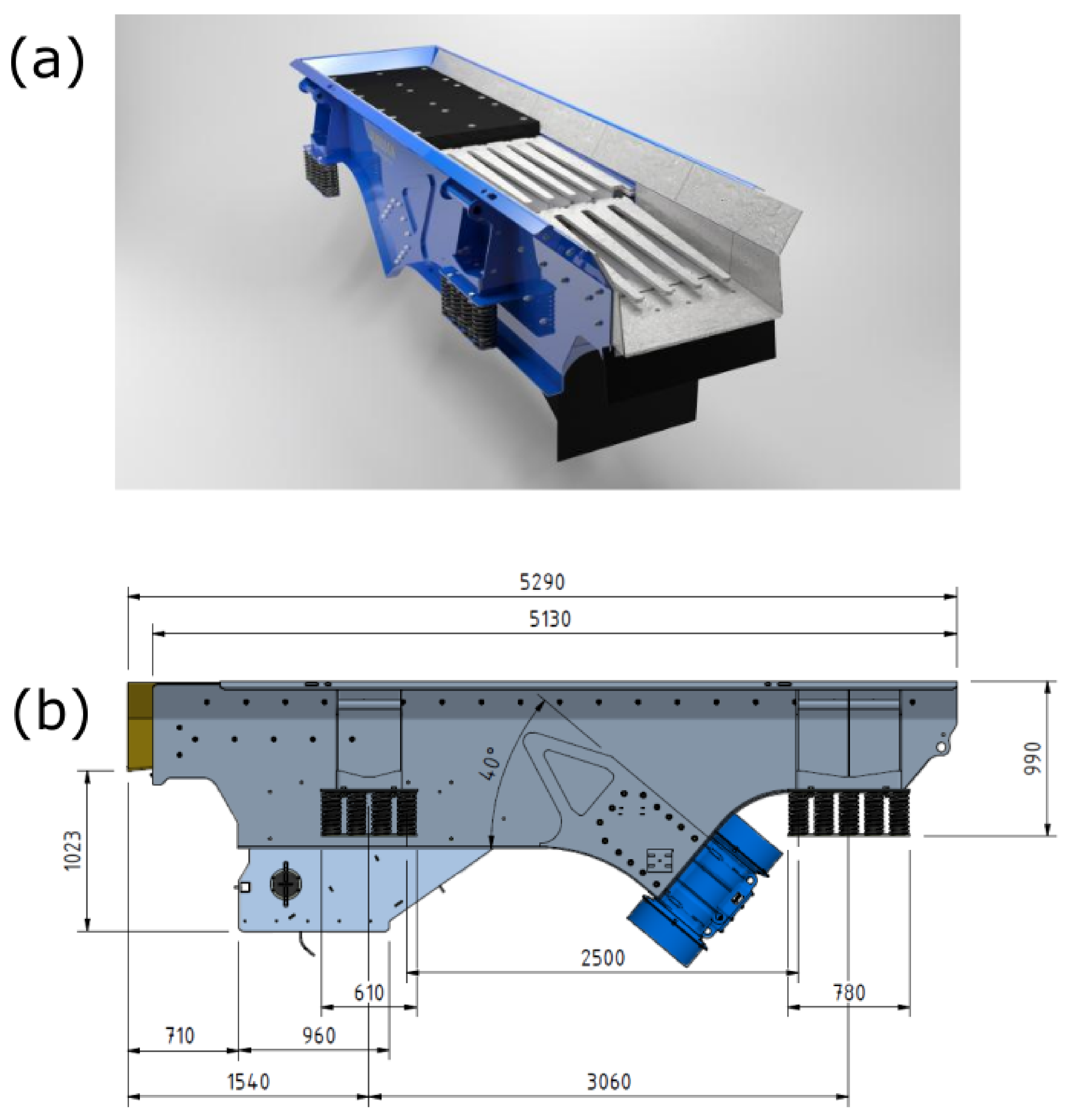
Figure 2.
(a) Showing a 3D picture of the P.J Jonsson feeder. The grizzlies (looks like teeth) observed are not present in the feeder in the present study. Instead, only steel plates are used. Overall dimensions can be seen in (b), the length of the feeder is 5.3 m and the width is 1.8 m. The direction of movement is 40° from the horizontal plane as observed in the figure. Pictures adopted from P.J Jonsson with permission.

Figure 3.
The Hardox 450 wear plates location on the feeder is shown (a). A close up look on the plates (b) are seen from behind and the dimensions for one plate are given.
Figure 3.
The Hardox 450 wear plates location on the feeder is shown (a). A close up look on the plates (b) are seen from behind and the dimensions for one plate are given.

Figure 4.
A photograph showing the 43 m large Esco bucket mounted on the Bucyrus electric rope shovel (ERS) in Aitik.
Figure 4.
A photograph showing the 43 m large Esco bucket mounted on the Bucyrus electric rope shovel (ERS) in Aitik.

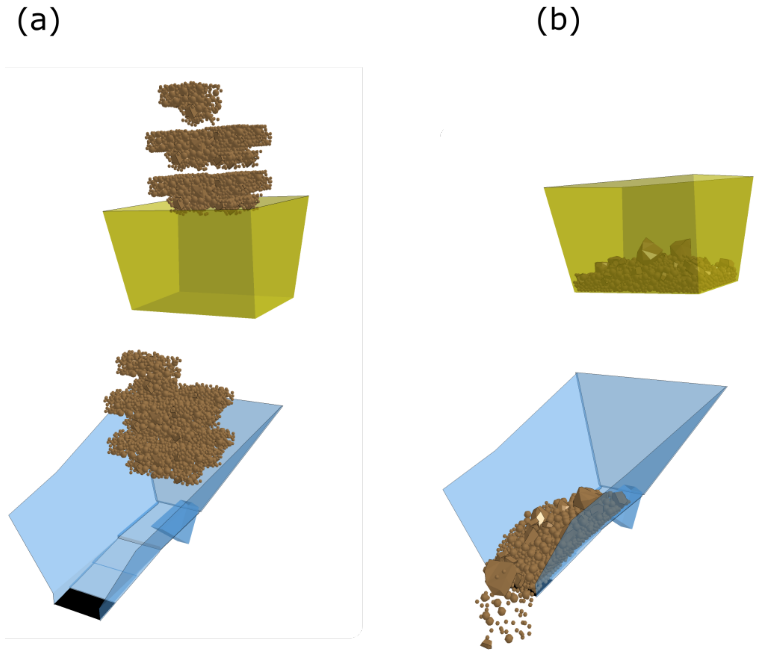
Figure 5.
Presentation of the simulation model setup for the feeder. The initial setup (a), and after several seconds into the simulation (b). The black area represents the plates where wear is measured.
Figure 5.
Presentation of the simulation model setup for the feeder. The initial setup (a), and after several seconds into the simulation (b). The black area represents the plates where wear is measured.

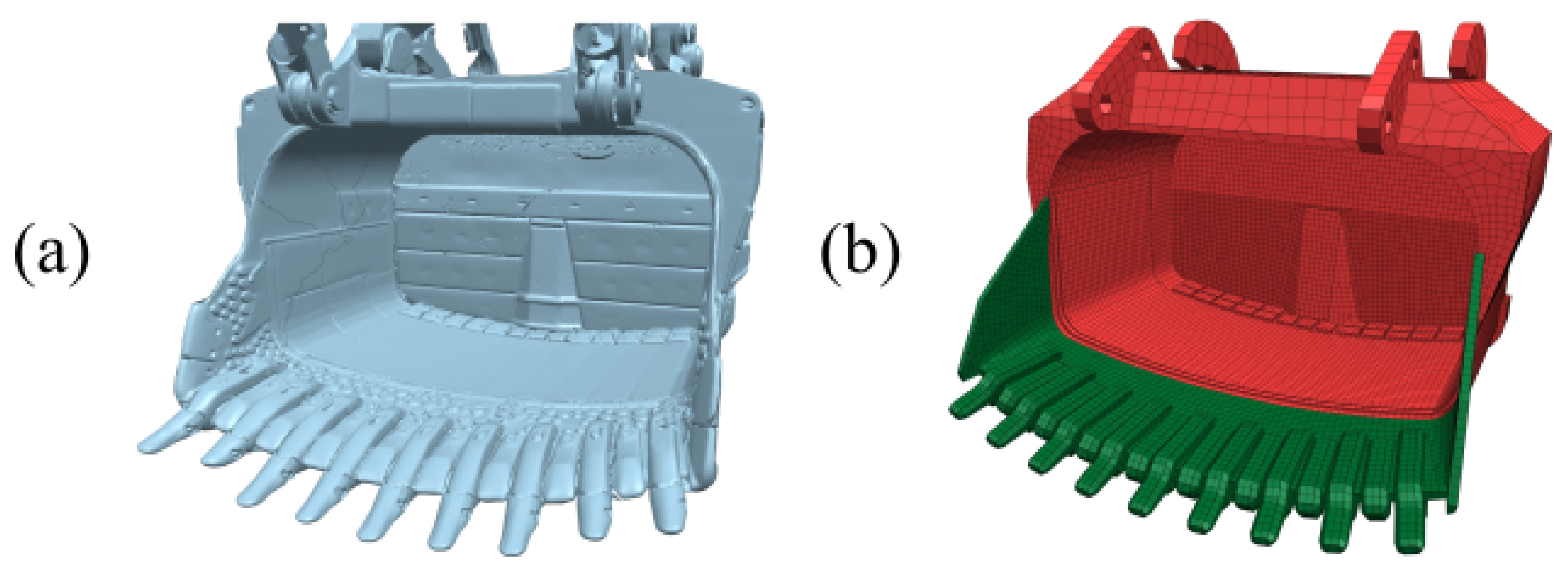
Figure 6.
Geometry and model of the Esco bucket. (a) 3D scanned bucket, (b) the FE-model.

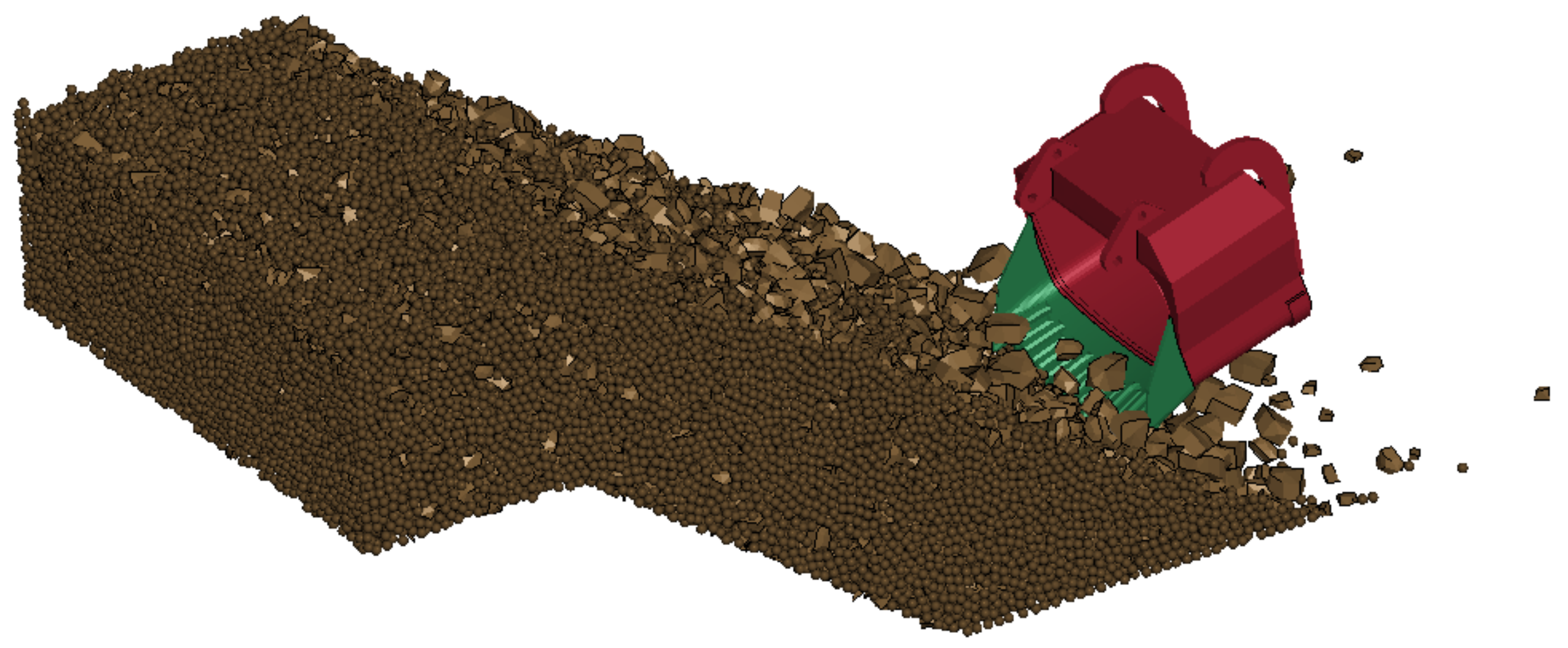
Figure 7.
Numerical model setup including the rigid body bucket and the granular material.

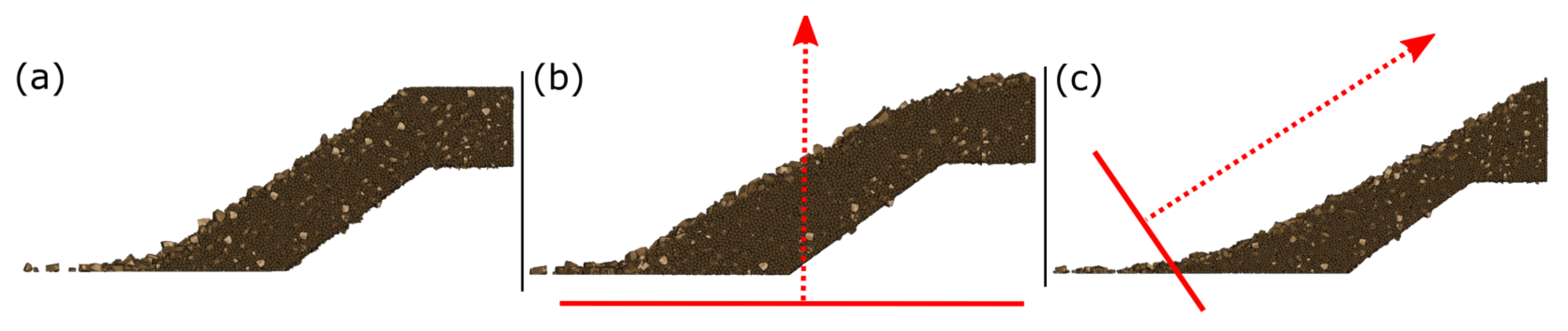
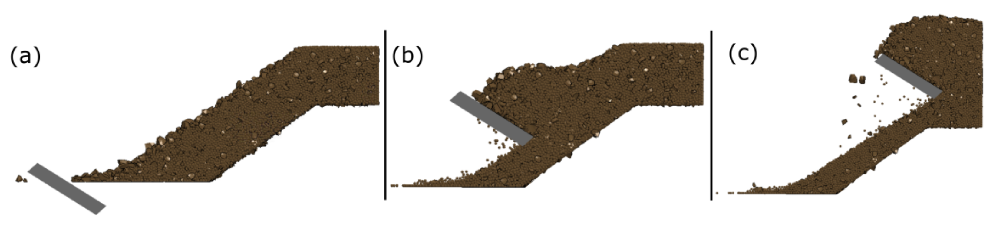
Figure 8.
A side view of the three different muck-piles. (a) the original muck-pile, rearrangement of the original muck-pile by moving a plate vertically (b), and at an angle (c). The thick line represents the plate, and the arrow the direction of movement.
Figure 8.
A side view of the three different muck-piles. (a) the original muck-pile, rearrangement of the original muck-pile by moving a plate vertically (b), and at an angle (c). The thick line represents the plate, and the arrow the direction of movement.

Figure 9.
Snapshots showing the creation of one muck-pile. A plate is moved across the muck pile (a–c). After the bucket has reached the top of the pile, the contact between the granular material and the plate is removed and the material flows due to gravity. The final pile is the one shown in Figure 8c.

Figure 10.
Geometry of the new buckets containing the steel bars at different angles. Bars at 90° (a) and bars at 45° (b) relative the direction of material flow.
Figure 10.
Geometry of the new buckets containing the steel bars at different angles. Bars at 90° (a) and bars at 45° (b) relative the direction of material flow.

Figure 11.
Plots showing the experimentally average wear depth for the plates described in Figure 3 as a function of the material feed passing the plates. The error bar represents the estimated error range from wear thickness measurements. is the wear rate between the different measurements.
Figure 11.
Plots showing the experimentally average wear depth for the plates described in Figure 3 as a function of the material feed passing the plates. The error bar represents the estimated error range from wear thickness measurements. is the wear rate between the different measurements.

Figure 12.
Absolute wear maps after calibration is performed for, (a) the PSD with smallest particles, radius, R = 50 mm, and (b) larger particles R = 100 mm, compared to the experimental results (c). x and y axes are the coordinates of the steel plates. The black dots represents the experimental coordinates where measuring of wear depth was performed. All units in mm.

Figure 13.
Figures showing normalized and mirror averaged wear maps for mesh edge lengths, (a) 30 mm, (b) 45 mm, (c) 60 mm, and (d) 75 mm. The particle size distribution is the smaller one with radius, R = 50 mm. Color plots are showing the normalized wear depth in mm.
Figure 13.
Figures showing normalized and mirror averaged wear maps for mesh edge lengths, (a) 30 mm, (b) 45 mm, (c) 60 mm, and (d) 75 mm. The particle size distribution is the smaller one with radius, R = 50 mm. Color plots are showing the normalized wear depth in mm.

Figure 14.
Figures showing normalized and mirror averaged wear maps for mesh edge lengths, (a) 30 mm, (b) 45 mm, (c) 60 mm, and (d) 75 mm. The particle size distribution is the baseline with smallest particles with radius, R = 100 mm. Color plots are showing the normalized wear depth in mm.
Figure 14.
Figures showing normalized and mirror averaged wear maps for mesh edge lengths, (a) 30 mm, (b) 45 mm, (c) 60 mm, and (d) 75 mm. The particle size distribution is the baseline with smallest particles with radius, R = 100 mm. Color plots are showing the normalized wear depth in mm.

Figure 15.
Normalized and mirror averaged wear maps for different amount of smoothings, (a) no smoothing iteration, (b) one smoothing iteration, (c) two smoothing iterations, and (d) three smoothing iterations. The mesh size was 75 mm, and the baseline case particles are used. Color plots are showing the normalized wear depth in mm.

Figure 16.
Snapshots from wear simulations during one bucket filling. In column (a), the wear is fringe plotted, and in column (b), a section view of the bucket and the granular material is shown for the different times.
Figure 16.
Snapshots from wear simulations during one bucket filling. In column (a), the wear is fringe plotted, and in column (b), a section view of the bucket and the granular material is shown for the different times.

Figure 17.
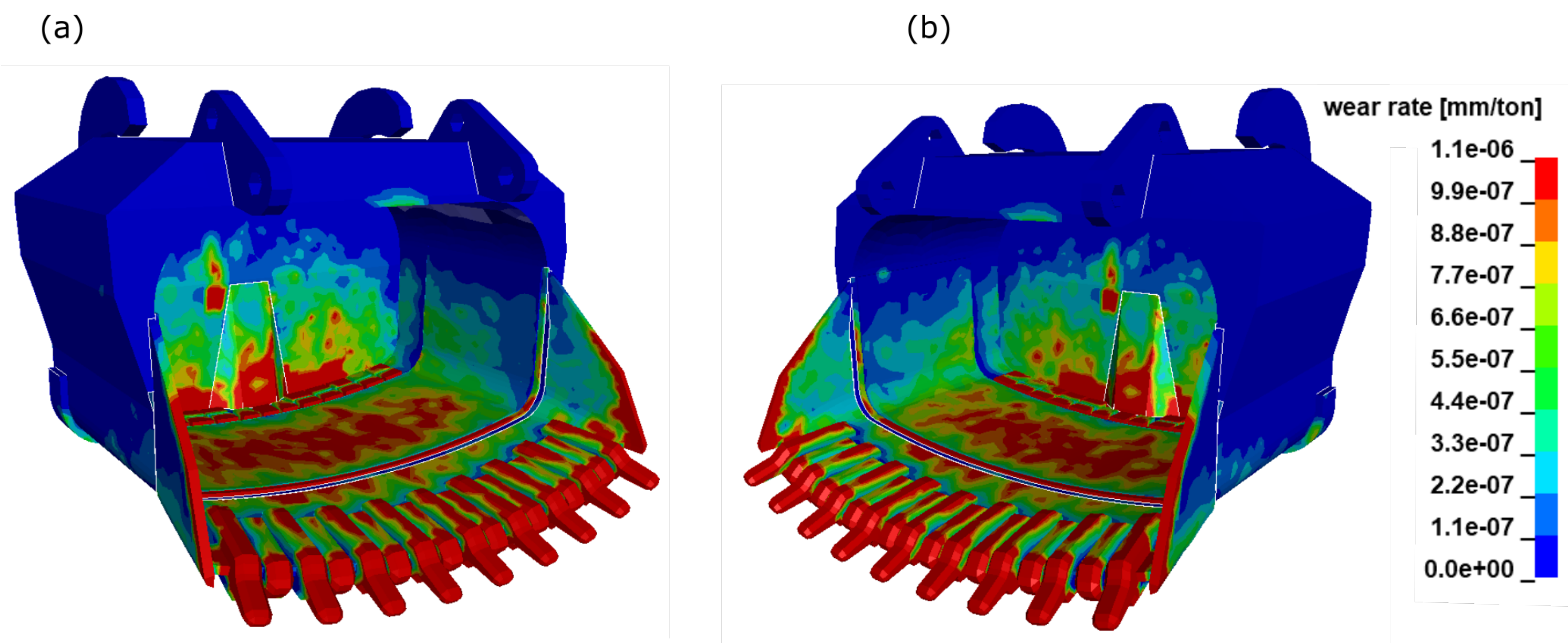
Overview of the predicted wear from simulations. View from (a) left, and (b) right. The color plots are in units mm/ton.
Figure 17.
Overview of the predicted wear from simulations. View from (a) left, and (b) right. The color plots are in units mm/ton.

Figure 18.
Figures showing the simulated (a) and experimental (b) wear rate. The wear maps are located at the bottom of the bucket (c). The lower parts of the wear maps correspond to the inlet of the bucket. The black markers in (b) correspond to the positions of the experimental measurements. The color plots are in units mm/ton.

Figure 19.
Wear rate is plotted as sections from the width direction of the bucket and plotted for both experimentally measured and simulated wear, in the front (a), middle (b), and in the rear of the bucket (c). The locations (d) of the sections in the bucket are illustrated. Experimental data are from the points in Figure 18, corresponding to approximately the same positions. The dashed line corresponds to experimental wear rate and the full drawn line corresponds to simulated wear rate. The x-axes are the same for all plots (a–c).

Figure 20.
Wear on the bottom and the lip of the bucket shown for the baseline case (a), the changed geometry with wear bars located at 90°, (b) and wear bars located at 45° (c). The changed geometries of the buckets are presented in Figure 10. The view is from the top, similar to the view in Figure 18. The units of the wear rate is mm/ton and the color plots are the same for all figures.

Figure 21.
Resultant contact interface forces acting on the bucket (excluding lip) for the baseline bucket and the buckets with added features. The average forces are 4.2 MN, 8.0 MN, and 6.8 MN, for the baseline case, wear bars at 90°, and for the wear bars at 45°, respectively. In Figure 16, the locations of the buckets at different times during the bucket filling are presented.


Table 1.
Physical properties for the DEM granular material model. The parameters were obtained in previous work [38].
Table 1.
Physical properties for the DEM granular material model. The parameters were obtained in previous work [38].
| Property | Parameter | Unit | Value |
|---|---|---|---|
| Time step | [s] | 4.5 × 10⁻⁵ | |
| Density | [kg/m] | 3700 | |
| Bulk density | [kg/m] | 1903 | |
| Young’s modulus | E | [GPa] | 45 |
| Poisson’s ratio | [-] | 0.3 | |
| DE-DE | |||
| Sliding fric. coeff. | [-] | 0.9 | |
| Rolling fric. coeff. | [-] | 0.05 | |
| Norm. damp. coeff. | [-] | 0.9 | |
| Tang. damp. coeff. | [-] | 0.75 | |
| DE-FE | |||
| Bucket-DE, sliding fric. coeff. | [-] | 0.53 | |
| Bucket-DE, rolling fric. coeff. | [-] | 0.05 | |
| FE rocks-DE, fric. coeffs | [-] | 0.85 | |
| Ground-DE, sliding fric. coeff. | [-] | 0.9 | |
| Ground-DE, rolling fric. coeff. | [-] | 0.3 | |
| FE-FE | |||
| FE rocks-FE rocks, fric. coeff. | [-] | 0.85 | |
| FE rocks-bucket, fric. coeff. | [-] | 0.53 | |
| FE rocks-ground fric. coeffs | [-] | 0.9 |
Publisher’s Note: MDPI stays neutral with regard to jurisdictional claims in published maps and institutional affiliations. |
© 2021 by the authors. Licensee MDPI, Basel, Switzerland. This article is an open access article distributed under the terms and conditions of the Creative Commons Attribution (CC BY) license (https://creativecommons.org/licenses/by/4.0/).
Share and Cite
MDPI and ACS Style
Svanberg, A.; Larsson, S.; Mäki, R.; Jonsén, P. Full-Scale Simulation and Validation of Wear for a Mining Rope Shovel Bucket. Minerals 2021, 11, 623. https://0-doi-org.brum.beds.ac.uk/10.3390/min11060623
AMA Style
Svanberg A, Larsson S, Mäki R, Jonsén P. Full-Scale Simulation and Validation of Wear for a Mining Rope Shovel Bucket. Minerals. 2021; 11(6):623. https://0-doi-org.brum.beds.ac.uk/10.3390/min11060623
Chicago/Turabian StyleSvanberg, Andreas, Simon Larsson, Rikard Mäki, and Pär Jonsén. 2021. "Full-Scale Simulation and Validation of Wear for a Mining Rope Shovel Bucket" Minerals 11, no. 6: 623. https://0-doi-org.brum.beds.ac.uk/10.3390/min11060623
Note that from the first issue of 2016, this journal uses article numbers instead of page numbers. See further details here.