
Delay-Dependent Stability, Integrability and Boundedeness Criteria for Delay Differential Systems


1
Department of Computer Programing, Baskale Vocational School, Van Yuzuncu Yil University, Van 65080, Turkey
2
Department of Mathematics, Faculty of Sciences, Van Yuzuncu Yil University, Van 65080, Turkey
3
Department of Mathematics, Zhejiang Normal University, Jinhua 321004, China
*
Author to whom correspondence should be addressed.
Axioms 2021, 10(3), 138; https://0-doi-org.brum.beds.ac.uk/10.3390/axioms10030138
Submission received: 30 April 2021
/
Revised: 11 June 2021
/
Accepted: 23 June 2021
/
Published: 29 June 2021
(This article belongs to the Special Issue Special Issue in Honor of the 60th Birthday of Professor Hong-Kun Xu)
Abstract
:This paper deals with non-perturbed and perturbed systems of nonlinear differential systems of first order with multiple time-varying delays. Here, for the considered systems, easily verifiable and applicable uniformly asymptotic stability, integrability, and boundedness criteria are obtained via defining an appropriate Lyapunov–Krasovskiĭ functional (LKF) and using the Lyapunov–Krasovskiĭ method (LKM). Comparisons with a former result that can be found in the literature illustrate the novelty of the stability theorem and show new contributions to the qualitative theory of solutions. A discussion of two illustrative examples and the obtained results are presented.
Keywords:
system of DDEs; uniformly asymptotically stability; integrability; boundedness at infinity; Lyapunov–Krasovskiĭ functional; multiple time-varying delayMSC:
34D05; 34K20; 26D15; 45J051. Introduction
The research of systems of delay differential equations (DDEs) with multiple constant and time-varying delays is always a challenging field of study. This is due to the fact that the system of DDEs can be frequently found in many fields such as mechanics, artificial neural networks power systems, medicine, physics, biology, population ecology, engineering, and so forth. For example, the books of Burton [1], Hale and Verduyn Lunel [2], Kiri and Ueda [3], Kolmanovskii and Myshkis [4], Kuang [5], Lakshmikantham et al. [6], and Smith [7] are very important reference books for various fundamental and qualitative results of stability and periodic solutions of functional differential equations of the first and second order. These books also include numerous methods, techniques, their theoretical and real applications in science, engineering, and technology. Indeed, a large number of applications in the theory of artificial neural networks, numerous models for some population dynamics, and ecology problems, etc., can be represented by DDEs with multiple delays, (see, in particular, Berezansky et al. [8], Gil [9], Smith [7], and the bibliography therein). Accordingly, the study of qualitative properties of solutions of scalar DDEs and systems of DDEs with multiple time-varying delays has an important significance in sciences and engineering, and it deserves the attention of researchers.
In recent years, numerous interesting and fruitful results on the qualitative analyses for various differential equations of first and second order both with and without delay have been obtained by applying a linear matrix inequality (LMI) approach, the second Lyapunov method, the LKM, fixed point method, and so on. In particular, some related works on the subject can be summarized briefly as the following.
Berezansky et al. [8] considered a non-autonomous system of first order with time-varying delays. Via the M-matrix method, easily verifiable sufficient stability conditions for the system and its linear version are obtained in [8].
In Berezansky et al. [10], uniform exponential stability of linear systems of first order with time varying coefficients is studied. In [10], a new explicit result is derived with the proof based on the Bohl–Perron theorem. The resulting criterion has advantages over some previous ones.
In Gil [9], the author presents exponential stability results for a nonlinear system of differential equations of first order. Here, the author obtains sharp bounds for the solutions of the system and thus exponential stability can be determined without the use of Lyapunov functions.
Gözen and Tunç [11] investigate an exponential stabilization problem for a class of linear systems of first order with two variable delays. Via a suitable Lyapunov–Krasovskiĭ functional, Leibniz–Newton’s formula and linear matrix inequalities, the authors derive some new sufficient conditions for the exponential stability of the zero solution of the system.
Liu [12] studies a class of systems of non-autonomous differential equations of first order with multiple delays. In [12], under proper conditions, several criteria of global stability of a positive equilibrium are obtained.
In Matsunaga [13], for a linear delay differential system of the first order with two coefficients and one delay, some necessary and sufficient conditions on the asymptotic stability of a zero solution, which are composed of delay-dependent and delay-independent stability criteria, are established and the range of the delay is explicitly given.
In Ngoc [14], general nonlinear time-varying differential systems of a first order with two variable delays are considered. Several explicit criteria for exponential stability are given. A discussion of the obtained results and two illustrative examples are presented.
In Petruşel et al. [15], existence, stability, and localization results for a general system of operator equations in complete metric spaces are presented. The approach is based on the application of some fixed point theorems for orbital contractions in a complete metric space.
In Rebenda and Šmarda [16], asymptotic properties of a real two-dimensional differential system with unbounded non-constant delays are investigated. The sufficient conditions for the stability and asymptotic stability of solutions are given. Asymptotic properties of solutions are also studied by means of a Lyapunov–Krasovskiĭ functional.
Shu [17] considers the linear delay system:
The author gives sufficient conditions for the asymptotic stability of the zero solution of this system by deriving a pair of one dimensional delay differential equations from the system and comparing the Lyapunov exponents of the corresponding fundamental solution.
Slyn’ko and Tunç [18] discusses the instability of set differential equations by using some geometric inequalities.
In Tunç [19,20,21] and Tunç and Tunç [22,23,24,25], stability, boundedness, and some other properties of solutions of various non-linear differential systems of second order without or with delay are investigated by the second Lyapunov method and integration techniques.
In Tunç and Golmankhaneh [26], the stability of fractal differentials in the sense of Lyapunov is defined. Sufficient conditions for the stability, uniform boundedness, and convergence of solutions for the suggested fractal differential equations are presented and proven.
Yskak [27] considers a class of linear systems of differential equations of first order with distributed delay and periodic coefficients. The author established sufficient conditions for the asymptotic stability of solutions to this system, obtain estimates of solutions, and study robust stability. On the basis of the obtained results, the author proves an analogue of the Krein’s theorem on stability of solutions to the linear system of differential equations with distributed delay.
In Zhang and Jiang [28], by constructing a suitable Lyapunov functional and using some analytical techniques, the authors obtain sufficient conditions for the global exponential stability of zero solution to a class of differential systems of first order with delay. The results show a relation between the delay time and the coefficients of the equations. In [28], two examples also are given to illustrate the validity of the results.
In Zhang and Wu [29], the authors develop a new technique to study the stability of the delay differential system of first order. In this way, the construction of suitable functionals for a given system with finite delay is easier. The conditions obtained are less restrictive. The main results are three theorems on the stability of the zero solution of the system with finite delay. We also refer readers to the papers of Petruşel and Rus [30], Kien et al. [31], Chadli et al. [32] and the bibliographies of the mentioned sources.
However, to the best of our knowledge, the LKM is the most effective method to investigate various properties of systems of delay DDEs with multiple time-varying delays provided that construct or define a suitable LKF. In fact, from this point of view, constructing, defining, or finding a suitable LKF for a problem under study is a difficult task and an unsolved problem in the literature until this time.
In 2020, Ren and Tian [33] considered the following system of linear DDEs with time-varying delay,
where is the system state, , and is the time-varying delay and satisfies the following conditions:
Ren and Tian [33] defined a LKF for the system of DDEs (1). Then, based upon the defined LKF, Ren and Tian [33] proved a theorem, ([33], Theorem 1), on the asymptotically stability of the system of DDEs (1).
The motivation of the results of this paper has been inspired from the paper of Ren and Tian ([33], Theorem 1) and those in the bibliography of this paper. In this paper, we take into consideration a perturbed nonlinear system of DDEs with three multiple time-varying delays as given below:
where , , , and are the time-varying delays, , , , and . We assume that the given time-varying delays and satisfy the following conditions:
We now outline the aim of this paper by the following items, respectively:
- (1)
- We study the uniformly asymptotic stability of zero solution and the integrability of the norm of solutions of the following unperturbed nonlinear system of DDEs via Theorem 3 and Theorem 4, respectively:To investigate these problems, we define a very different LKF from that in Ren and Tian [16];
- (2)
- We investigate the boundedness of solutions of the perturbed system of nonlinear DDEs (2), see Theorem 5’
- (3)
- In particular cases, two new examples with graphs of their solutions are provided to show applications of Theorems 3–5.
The rest of this paper is organized as follows. Some basic information related to a general functional differential system and a necessary auxiliary theorem, Burton ([1], Theorem 4.2.9), are given in Section 2. A reference theorem of this paper, Ren and Tian ([33], Theorem 1), concerning asymptotic stability of the system of linear DDEs (1) is given in Section 3. Two new results and an example concerning uniformly asymptotic stability and integrability for the unperturbed system (4) are presented in Section 4, while a result and an example for the boundedness of solutions of the perturbed system of DDEs (2) are given in Section 5. Finally, some discussions, contributions, and a conclusion are given in Section 6 and Section 7, respectively.
2. Background and Motivation
Consider the system of DDEs:
where , and takes bounded sets into bounded sets. For some , denotes the space of continuous functions . For any , and , we have for and .
Let . The norm is defined by . Next, let . For this case, the matrix norm, , is defined by .
In this article, without loss of generality, sometimes instead of , we will simply write x.
For any , let:
and
We suppose that the function H satisfies the conditions of the uniqueness of solutions of the system of DDEs (5). We note that the system of DDEs (2) is a particular case of the system of DDEs (5).
Let be a solution of the system of DDEs (5) such that on , where is an initial function.
Let,
be a continuous functional in t and with . Further, let denote the derivative of on the right through any solution of the system of DDEs (5).
Theorem 1
(Burton ([1], Theorem 4.2.9). Assume that:
- (A1)
- The functionsatisfies the locally Lipschitz in x, i.e., for every compactand, there exists awithsuch that:for alland;
- (A2)
- Letbe a functional such that it satisfies the one-side locally Lipschitz in t:whenever, whereis continuous;
- (A3)
- There are four strictly increasing functions ω,,,with value 0 at 0 such that:andwheneverand. Then, the solutionof the system of DDEs (5) is uniformly asymptotically stable.
3. Asymptotic Stability
Firstly, we state the main result of Ren and Tian ([33], Theorem 1).
Theorem 2
(Ren and Tian [33], Theorem 1). For given scalars and , the system (1) with time-varying delays satisfying the condition is asymptotically stable if there exist matrices ,
, such that the LMI:
holds forwhere:
and
is defined as:
4. Uniformly Asymptotic Stability and Integrability
We now deal with the non-perturbed system of DDEs (4). Here, we first extend and optimize the asymptotic stability result of Ren and Tian ([33], Theorem 1) under very weaker conditions. Next, we give an integrability result for the solutions of the unperturbed non-linear system of DDEs (4). The technique of the proofs is based upon the LKM.
The first main result of this paper is given by Theorem 3.
Theorem 3.
We assume that the following conditions (C1) and (C2) hold:
- (C1)
- There exist positive constants,, andsuch that:and
- (C2)
- There exist constants, ,andfrom (C1) and (2), respectively, andsuch that:Then zero solution of the unperturbed system of DDEs (4) is uniformly asymptotically stable.
Proof.
We define a new LKF by:
where , such that these arbitrary constants will be chosen in the proof later.
The LKF (6) can be expanded as the following:
From (6), it follows that the LKF satisfies:
Let,
and
Hence, it is clear that:
As for the next step, by some elementary calculations, we derive:
From this point of view, we have:
where:
Thus, we can conclude that:
The last inequality shows that the LKF satisfies the locally Lipschitz condition. Hence, the satisfaction of the condition (A1) of Burton ([1], Theorem 4. 2.9) was shown.
For the next step, from the definition of , it follows that:
Thus, we get:
As for the next step, using some simple calculations, we find:
where:
Thus, the satisfaction of the condition (A2) of Burton ([1], Theorem 4. 2.9) was proven.
As for the next step, we calculate the time derivative of the LKF in (6) along the system of DDEs (4). Then, we can obtain that:
We now consider the first term of the equality (7). Via the condition (C1) and some elementary calculations, we have that:
From this point of view, combining (7) and (8) and using the conditions of (3), it follows that:
Since and are arbitrary positive constants, let and . Then, keeping in the mind the condition (C2), we conclude that:
where:
Hence, from (9), it is seen that the derivative is negative definite. Thus, the condition (A3) of Burton ([1], Theorem 4. 2.9) was satisfied. Hence, all the conditions of (A1)–(A3) of Burton ([1], Theorem 4. 2.9) were satisfied. The whole discussion proves that the zero solution of the nonlinear unperturbed system of DDEs (4) with two multiple time-varying delays is uniformly asymptotically stable. This completes the proof of Theorem 3. □
Theorem 4.
Let the conditions (C1) and (C2) of Theorem 3 hold. Then the norm of solutions of the unperturbed system of DDEs (4) with two multiple time-varying delays are integrable in the sense of Lebesgue on.
Proof.
The proof of this theorem depends upon the LKF . Via the conditions (C1) and (C2), as before we obtain the inequality:
Since is negative definite, the LKF is decreasing. Keeping in mind this fact and integrating the inequality (10), we obtain:
for all . This inequality clearly implies:
□
Thus, the norm of the solutions of the unperturbed system of DDEs (4) with multiple two time-varying delays is integrable in the sense of Lebesgue on . Hence, the proof of Theorem 4 is completed.
In a particular case of the unperturbed system of DDEs (4) with two multiple time-varying delays, we now give an example, Example 1, to show that the conditions of (C1) and (C2) of Theorem 3 and Theorem 4 can hold.
Example 1.
Consider the following system of non-linear DDEs with two multiple time-varying delays:
whereandare two multiple time-varying delays, and.
From this point of view, we compare both the system of DDEs (11) and DDEs (4) with two multiple time-varying delays. Hence, we derive that:
Let,
and
In view of the matrix , it is clear that:
Then,
Next, by some simple calculations, we obtain:
and
Assume that:
Considering the statement of condition (C2) and the above calculations, we have:
From this point of view, it follows that all the conditions of Theorems 3 and 4, i.e., the conditions (C1) and (C2) hold. For this reason, the zero solution of the system of DDEs (11) with two multiple time-varying delays is uniformly asymptotic stable as well as the norm of solutions of the same system are integrable.
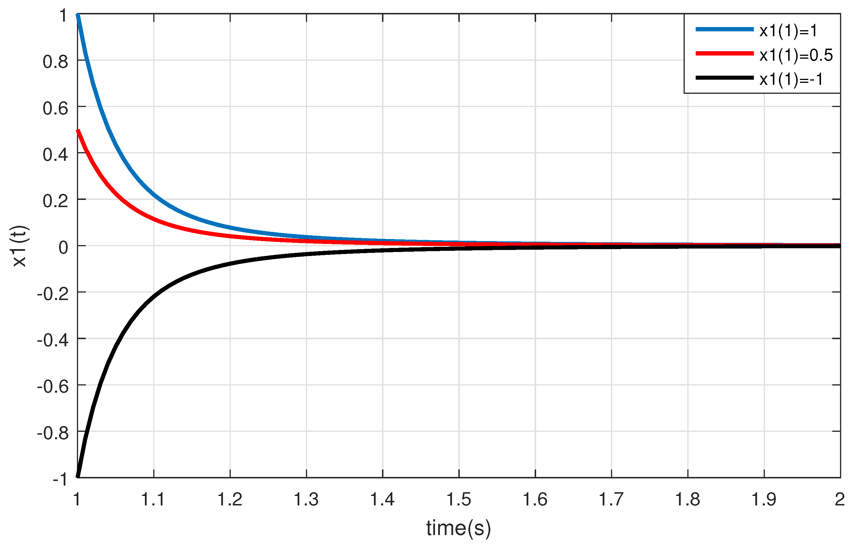
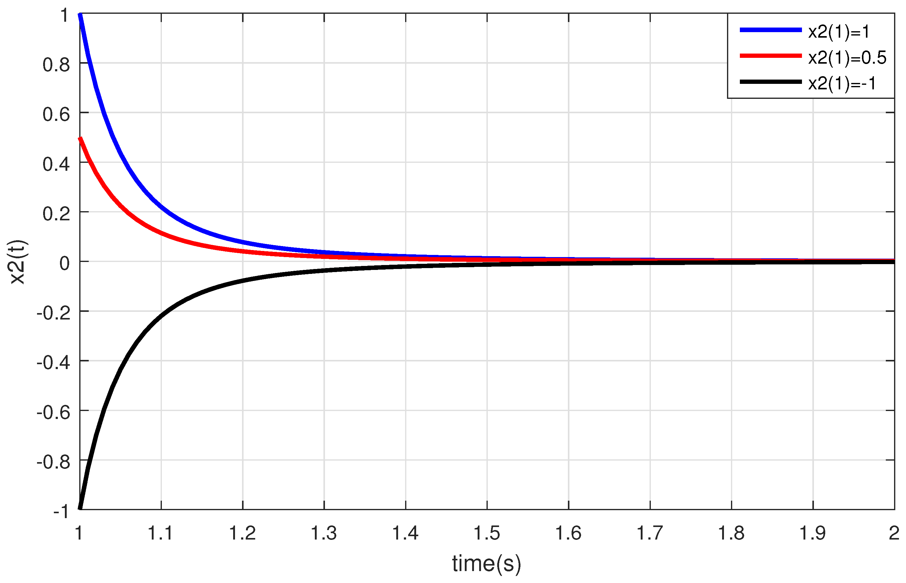
Here, Example 1 was solved using MATLAB software. Indeed, the given example was solved using the 4th order Runge–Kutta method in MATLAB. The graphs of Figure 1 and Figure 2 show the behaviors of paths of the solutions of Example 1, respectively, for , , , and different initial values.
We now present our third main result of this paper related to the boundedness of solutions of the perturbed nonlinear system of DDEs (2) with three multiple time-varying delays.
5. Boundedness of Solutions
For the boundedness of solutions of the perturbed system of DDEs (2) with three multiple time-varying delays, in addition to the conditions (C1) and (C2), we need the following condition:
- (C3)
- There exist positive constants , , , , from (C1) and (C2), L and a continuous function such that:where:
Theorem 5.
Let conditions (C1)–(C3) hold. Then the solutions of the perturbed system of DDEs (2) with three multiple time-varying delays are bounded as.
Proof.
As in the previous theorems, the proof of this theorem also depends upon the LKF . From the conditions (C1)–(C3), we can derive:
□
Integrating the inequality (12) and using the condition (C3), we obtain that:
Let,
Using (13) and the definition of the LKF , we have:
i.e.,
By calculating the limit of this inequality as , it is derived that:
Then, we can conclude that the solutions of the perturbed system of nonlinear DDEs (2) with three multiple time-varying delays are bounded as . Thus, Theorem 5 is proven.
In a particular case of the perturbed system of DDEs (2) with three multiple time-varying delays, we now give Example 2, to show that the conditions of (C1)–(C3) of Theorem 5 can be provided.
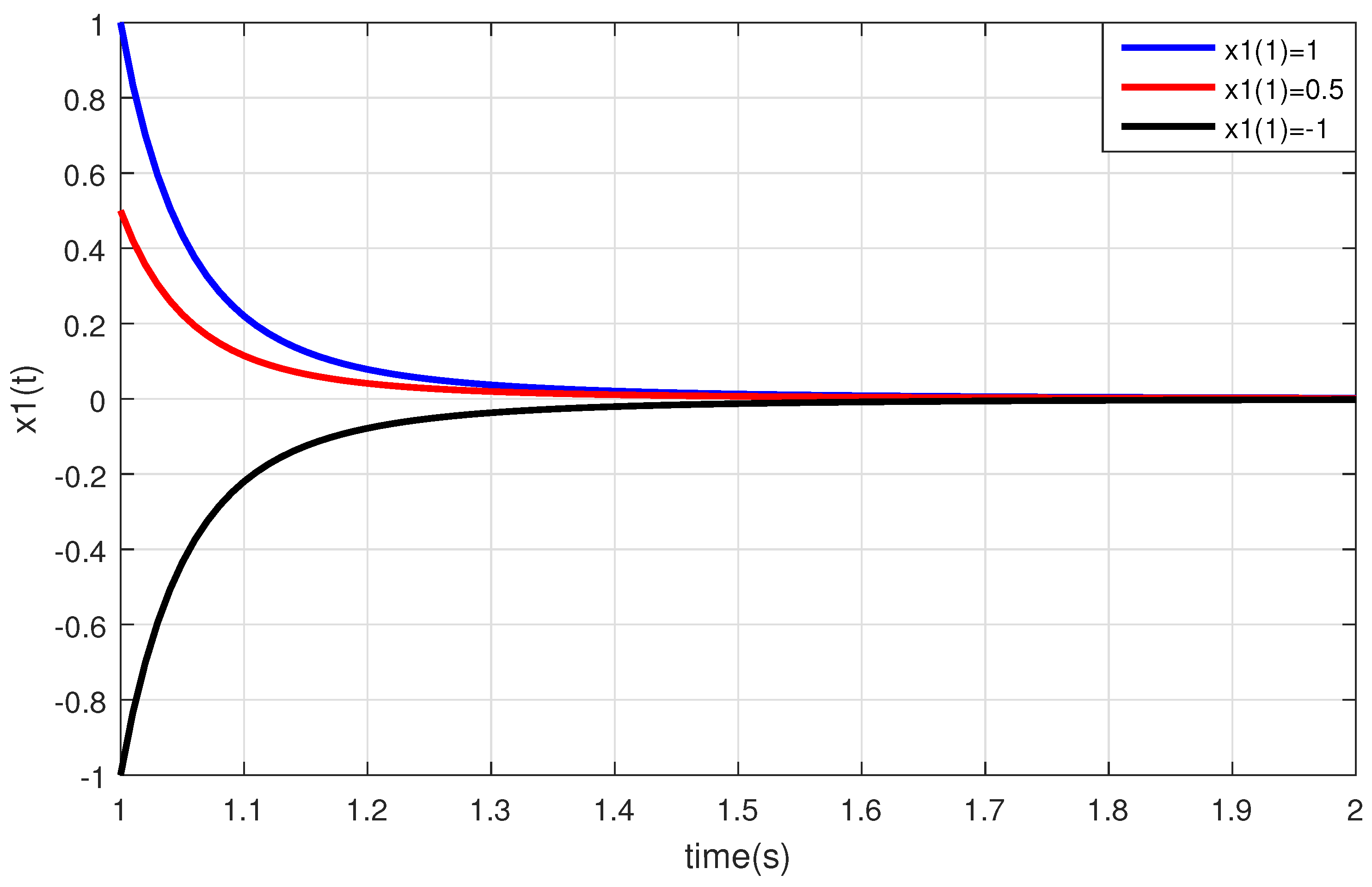
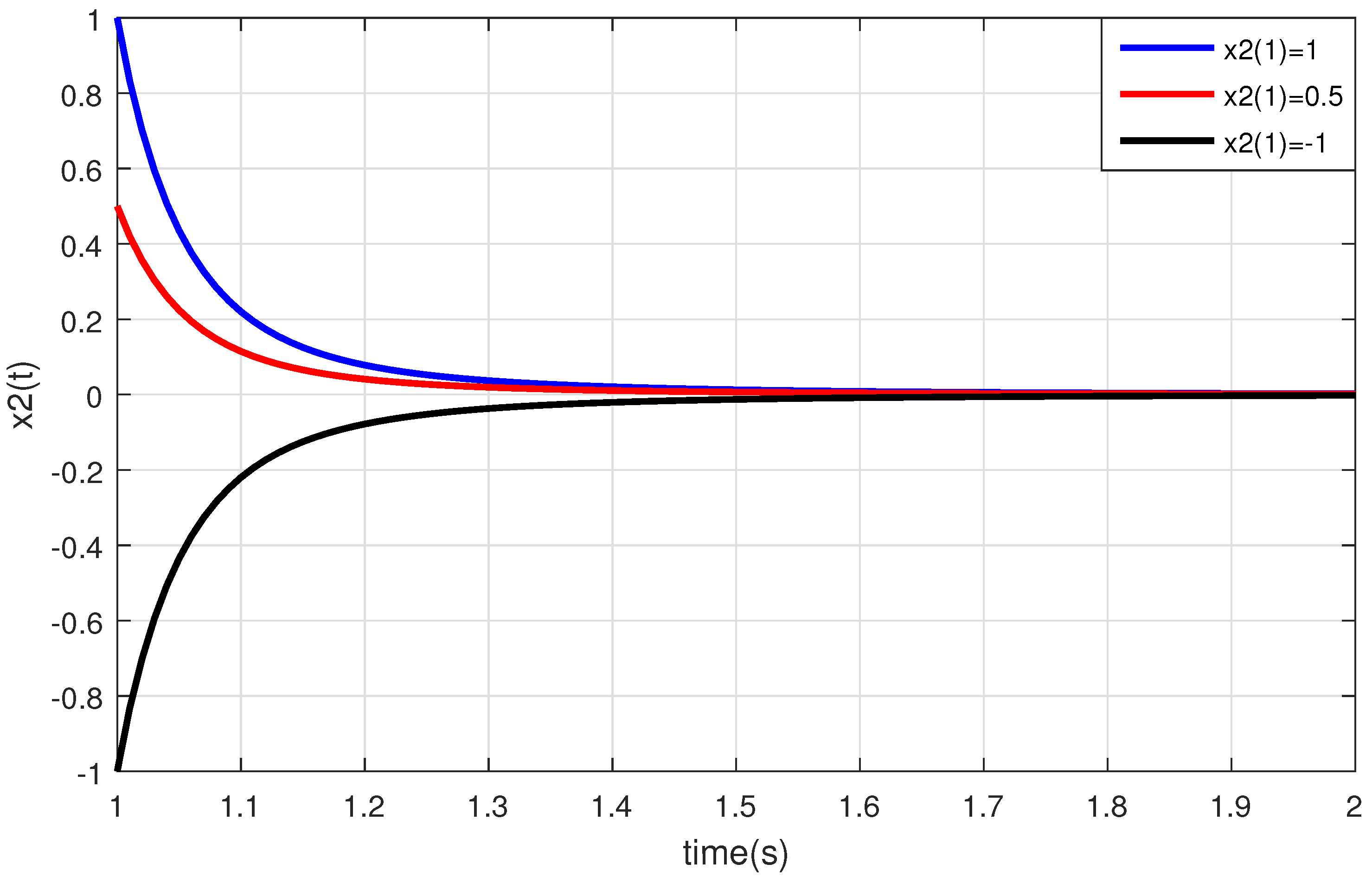
Here, Example 2 was solved using MATLAB software. Indeed, the given example was solved using the 4th order Runge–Kutta method in MATLAB. The graphs of Figure 3 and Figure 4 show the behaviors of paths of the solutions of Examples 2, respectively, for , , , and different initial values.
Example 2.
Consider the following nonlinear system of DDEs with three multiple time-varying delays:
where,, andare three multiple time-varying delays, and.
If nonlinear system of DDEs (14) and the perturbed system of DDEs (2) with three multiple time-varying delays are compared, then the condition (C1) and (C2) are satisfied, since they were shown in Example 1. As for the condition (C3), it is clear that:
From this point of view, we derive that:
where:
Hence, we obtain:
The obtained results shows that the conditions of (C1)–(C3) of Theorem 5 can hold. Thus, all the solutions of the nonlinear system of DDEs (14) with three multiple time-varying delays are bounded as .
6. Discussion and Contribution
We first compare the conditions Theorems 3 with those of the main result of Ren and Tian ([33], Theorem 1). We also explain the contributions of the next two results, Theorems 4 and 5, of this paper to the relevant literature by the following items, respectively.
- (1)
- The nonlinear perturbed system of DDEs (2) extend and improve the linear system of DDEs (1) (see Tian and Ren [33], Theorem 1) from a linear system of the DDEs with a time-varying delay to the a class of non-linear systems of DDEs with three multiple time-varying delays. Next, in the main result of Tian and Ren ([33], Theorem 1), see the above Theorem 2, the satisfaction of the following LMI is very difficult:since the matrix has numerous terms. This fact can be seen clearly, when we look at ([33], Theorem 1) and the above Theorem 2. Hence, it is clear that this condition can lead conservatism, computational complexity, and difficulty in application fields. However, here, we have very simple conditions, (C1) and (C2) for our stronger result of uniformly asymptotically stability, Theorem 3, instead of asymptotically stability result in ([33], Theorem 1). For sake of brevity, there is no need for more information
- (2)
- To prove Theorem 1, the following LKF ,withis defined by Ren and Tian ([33], Theorem 1). Instead of the LKF (15), we defined the following LKF:In spite of the non-linear unperturbed system of DDEs (2) having three multiple time-varying delays, the LKF (16) is very simple and more convenient and effective. For the particular case of our theorem, Theorem 3, to get the main result of Ren and Tian ([33], Theorem 1) under very less conservative and optimal conditions, we need the following LKF:which is a particular case of the LKF (16).
- (3)
- In Ren and Tian ([33], Theorem 1), differentiating the LKF (15) and using the system of DDEs (1), it was derived that:withHowever, let . It is interesting that calculating the time derivative of the LKF given by (17) and using the system of DDEs (1), we obtain:The equality (20) has a very simple form than those given by (18) and (19). Indeed, the inequality (20) leads very to less conservative conditions for the negative definiteness of the time derivative than those given by Ren and Tian ([33], Theorem 1) for the negative definiteness of . Here, we would not like to give the details of the discussions for the sake of brevity. The less restrictive conditions of Theorem 3 can be followed with a comparison made between the conditions of Ren and Tian ([33], Theorem 1) and our Theorem 3.
- (4)
- To prove Theorem 2, which is given above, firstly, three lemmas, Lemmas 1–3, are given by Ren and Tian [33]. Then, based upon the integral and matrix inequalities therein, a new delay-dependent stability criterion via Theorem 2 is proven in terms of a linear matrix inequality, see Ren and Tian [33], Theorem 1.In this paper, we define a more suitable LKF (6) and depend upon Burton [1], (Theorem 4. 2.9), to prove Theorems 3–5. From this point of view, Ren and Tian ([33], Theorem 1) investigated the asymptotic stability of the linear system of DDEs (1). Here, we investigate the uniformly asymptotically stability of the zero solution and integrability of the norm of solutions of an unperturbed system of DDEs (4) as well as the boundedness of solutions of the perturbed system of DDEs (2). The result of Theorem 3, the uniformly asymptotically stability includes and implies the asymptotic stability of the linear system of DDEs (1), i.e., but the converse is not true.As a brief summary, here, we extend and improve the result of Ren and Tian ([33], Theorem 1), and obtain this result under very less conservative conditions and make it more optimal than before. Next, we also obtain two new results on the qualitative properties of the nonlinear unperturbed system of DDEs (4) and as well as the nonlinear perturbed system of DDEs (2), (see Theorems 4 and 5). The applicability of our results can be done easily because of the form of the new less restrictive conditions of Theorems 3–5.
- (5)
- In this particular case, two nonlinear Examples 1 and 2 with two and three time-varying delays, respectively, are given. These examples satisfy the conditions of Theorems 3–5 and they were solved depending upon the 4th order Runge–Kutta method. The trajectories of these examples are plotted by MATLAB software. The stability, integrability, and boundedness of the solutions can be followed clearly.
- (6)
- An advantage of the new and optimal LKF (6) used in the proof of Theorem 5 is to eliminate using Gronwall’s inequality for the boundedness of solutions at infinity. A comparison of Theorems 3–5 and those in the literature also shows that the conditions of Theorems 3–5 are more general, simple, and convenient for applications.
7. Conclusions
In this paper, the unperturbed system of DDEs (4) with two multiple time-varying delays and the perturbed system of DDEs (2) with three multiple time-varying delays are taken into consideration. To the best of the authors’ knowledge, the qualitative properties of the systems of DDEs (2) and (4) with multiple time-varying delays were not investigated in the relevant literature until this time and the results of this article are new, original, and have scientific novelty.
Indeed, this paper is comprised of three new results, Theorems 3–5, and two new examples, Examples 1 and 2. Theorems 3–5 are related to the uniformly asymptotically stability of zero solution and the integrability of solutions of the non-perturbed system of DDEs (4) as well as the boundedness of solutions of the perturbed system of the DDEs (2), respectively. The technique used to prove Theorems 3–5 depends upon a new LKF and the LKF method. In fact, the real advantage of the new LKF is that it can pioneer to more optimal, general, and less conservative new qualitative results and also eliminate the use of Gronwall’s inequality for the boundedness of solutions.
The established sufficient conditions of Theorems 3–5 are more general, simple, less conservative, and more convenient to apply than those available from the literature.
The results of this paper also improve and extend the result of Ren and Tian ([33], Theorem 1) and add two new results on the qualitative properties of solutions and contributes to the topic and relevant literature. The given examples illustrate the particular applications of the new results of this paper.
Author Contributions
Conceptualization, O.T., C.T. and Y.W.; Data curation, O.T.; Formal analysis, O.T., C.T. and Y.W.; Funding acquisition, Y.W.; Methodology, C.T., O.T. and Y.W.; Project administration, C.T.; Supervision, Y.W. and O.T.; Validation, C.T., Y.W.; Visualization, O.T.; Writing—original draft, O.T. All authors have read and agreed to the published version of the manuscript.
Funding
This research was funded by the National Natural Science Foundation of China, grant number 11671365 and the Natural Science Foundation of Zhejiang Province, grant umber LY14A010011.
Institutional Review Board Statement
Not applicable.
Informed Consent Statement
Not applicable.
Data Availability Statement
Not applicable.
Acknowledgments
The authors would like to thank the handling editor and the anonymous referees for their many useful comments and suggestions leading to a substantial improvement of the presentation of this article.
Conflicts of Interest
The authors declare no conflict of interest.
References
- Burton, T.A. Stability and Periodic Solutions of Ordinary and Functional Differential Equations; Corrected Version of the 1985 Original; Dover Publications, Inc.: Mineola, NY, USA, 2005. [Google Scholar]
- Hale, J.K.; Lunel, S.M.V. Introduction to functional-differential equations. In Applied Mathematical Sciences; Springer: New York, NY, USA, 1993; p. 99. [Google Scholar]
- Kiri, Y.; Ueda, Y. Stability criteria for some system of delay differential equations. In Theory, Numerics and Applications of Hyperbolic Problems II; Springer Processing In Mathematics amd Statistics, 237; Springer: Cham, Switzerland, 2016; pp. 137–144. [Google Scholar]
- Kolmanovskii, V.; Myshkis, A. Applied theory of functional-differential equations. In Mathematics and Its Applications; Soviet Series 85; Kluwer Academic Publishers Group: Dordrecht, The Netherlands, 1992. [Google Scholar]
- Kuang, Y. Delay differential equations with applications in population dynamics. In Mathematics in Science and Engineering; Academic Press, Inc.: Boston, MA, USA, 1993; p. 191. [Google Scholar]
- Lakshmikantham, V.; Wen, L.Z.; Zhang, B.G. Theory of differential equations with unbounded delay. In Mathematics and Its Applications; Kluwer Academic Publishers Group: Dordrecht, The Netherlands, 1994; p. 298. [Google Scholar]
- Smith, H. An Introduction to Delay Differential Equations with Applications to the Life Sciences; Texts in Applied Mathematics 57; Springer: New York, NY, USA, 2011. [Google Scholar]
- Berezansky, L.; Braverman, E.; Idels, L. New global exponential stability criteria for nonlinear delay differential systems with applications to BAM neural networks. Appl. Math. Comput. 2014, 243, 899–910. [Google Scholar] [CrossRef] [Green Version]
- Gil’, M.I. Exponential stability of nonlinear non-autonomous multivariable systems. Discuss. Math. Differ. Incl. Control Optim. 2015, 35, 89–100. [Google Scholar] [CrossRef]
- Berezansky, L.; Diblík, J.; Svoboda, Z.; Šmarda, Z. Simple uniform exponential stability conditions for a system of linear delay differential equations. Appl. Math. Comput. 2015, 250, 605–614. [Google Scholar] [CrossRef]
- Gözen, M.; Tunç, C. A new result on exponential stability of a linear differential system of first order with variable delays. Nonlinear Stud. 2020, 27, 275–284. [Google Scholar]
- Liu, B. Global stability of a class of non-autonomous delay differential systems. Proc. Am. Math. Soc. 2010, 138, 975–985. [Google Scholar] [CrossRef] [Green Version]
- Matsunaga, H. Delay-dependent and delay-independent stability criteria for a delay differential system. Proc. Am. Math. Soc. 2008, 136, 4305–4312. [Google Scholar] [CrossRef]
- Ngoc, P.H.A. Stability of nonlinear differential systems with delay. Evol. Equ. Control Theory 2015, 4, 493–505. [Google Scholar] [CrossRef] [Green Version]
- Petruşel, A.; Petruxsxel, G.; Yao, J. Existence and stability results for a system of operator equations via fixed point theory for non-self orbital contractions. J. Fixed Point Theory Appl. 2019, 21, 18. [Google Scholar] [CrossRef]
- Rebenda, J.; Šmarda, Z. Stability of a functional differential system with a finite number of delays. Abstr. Appl. Anal. 2013, 2013, 853134. [Google Scholar] [CrossRef]
- Shu, F.C. Stability of a 2-dimensional irreducible linear system of delay differential equations. Appl. Math. E Notes 2012, 12, 36–43. [Google Scholar]
- Slyn’ko, V.I.; Tunç, C. Instability of set differential equations. J. Math. Anal. Appl. 2018, 467, 935–947. [Google Scholar] [CrossRef]
- Tunç, C. A note on boundedness of solutions to a class of non-autonomous differential equations of second order. Appl. Anal. Discrete Math. 2010, 4, 361–372. [Google Scholar] [CrossRef] [Green Version]
- Tunç, C. Uniformly stability and boundedness of solutions of second order nonlinear delay differential equations. Appl. Comput. Math. 2011, 10, 449–462. [Google Scholar]
- Tunç, C. Stability to vector Liénard equation with constant deviating argument. Nonlinear Dynam. 2013, 73, 1245–1251. [Google Scholar] [CrossRef]
- Tunç, C.; Tunç, O. A note on certain qualitative properties of a second order linear differential system. Appl. Math. Inf. Sci. 2015, 9, 953–956. [Google Scholar]
- Tunç, C.; Tunç, O. On the boundedness and integration of non-oscillatory solutions of certain linear differential equations of second order. J. Adv. Res. 2016, 7, 165–168. [Google Scholar] [CrossRef] [PubMed] [Green Version]
- Tunç, C.; Tunç, O. A note on the stability and boundedness of solutions to non-linear differential systems of second order. J. Assoc. Arab Univ. Basic Appl. Sci. 2017, 24, 169–175. [Google Scholar] [CrossRef]
- Tunç, C.; Tunç, O. Qualitative analysis for a variable delay system of differential equations of second order. J. Taibah Univ. Sci. 2019, 13, 468–477. [Google Scholar] [CrossRef] [Green Version]
- Tunç, C.; Golmankhaneh, A.K. On stability of a class of second alpha-order fractal differential equations. AIMS Math. 2020, 5, 2126–2142. [Google Scholar] [CrossRef]
- Yskak, T. Stability of solutions to systems of differential equations with distributed delay. Funct. Differ. Equ. 2018, 25, 97–108. [Google Scholar]
- Zhang, H.; Jiang, W. Global exponential stability to a class of differential system with delay. Ann. Differ. Equ. 2007, 23, 564–569. [Google Scholar]
- Zhang, S.; Wu, S. Stability of delay differential systems by several Liapunov functions. Ann. Differ. Equ. 2001, 17, 86–92. [Google Scholar]
- Petruşel, A.; Rus, I.A. The Ulam-Hyers stability of an ordinary differential equation via Gronwall lemmas. Appl. Set Valued Anal. Optim. 2020, 2, 295–303. [Google Scholar]
- Kien, B.T.; Qin, X.; Wen, C.F. L∞-stability for a class of parametric optimal control problems with mixed pointwise constraints. J. Appl. Numer. Optim. 2020, 2, 297–320. [Google Scholar]
- Chadli, O.; Koukkous, A.; Saidi, A. Existence of anti-periodic solutions for nonlinear implicit evolution equations with time dependent pseudomonotone operators. J. Nonlinear Var. Aanl. 2017, 1, 71–88. [Google Scholar]
- Ren, Z.; Tian, J. Stability analysis of systems with interval time-varying delays via a new integral inequality. Complexity 2020, 2020, 2854293. [Google Scholar] [CrossRef] [Green Version]
Figure 1.
This figure shows that the solution of the system of DDEs (11) with two multiple time-varying delays is uniformly asymptotically stable and the norm of this solution is integrable for , , , and different initial values.
Figure 1.
This figure shows that the solution of the system of DDEs (11) with two multiple time-varying delays is uniformly asymptotically stable and the norm of this solution is integrable for , , , and different initial values.

Figure 2.
This figure shows that the solution of the system of DDEs (11) with two multiple time-varying delays is uniformly asymptotically stable and the norm of this solution is integrable for , , , and different initial values.
Figure 2.
This figure shows that the solution of the system of DDEs (11) with two multiple time-varying delays is uniformly asymptotically stable and the norm of this solution is integrable for , , , and different initial values.

Figure 3.
This figure shows that the solution of the perturbed nonlinear system of DDEs (14) with three time-varying delays is bounded for , , , , and different initial values.
Figure 3.
This figure shows that the solution of the perturbed nonlinear system of DDEs (14) with three time-varying delays is bounded for , , , , and different initial values.

Figure 4.
This figure shows that the solution of the perturbed nonlinear system of DDEs (14) with three time-varying delays is bounded for , , , , and different initial values.
Figure 4.
This figure shows that the solution of the perturbed nonlinear system of DDEs (14) with three time-varying delays is bounded for , , , , and different initial values.

Publisher’s Note: MDPI stays neutral with regard to jurisdictional claims in published maps and institutional affiliations. |
© 2021 by the authors. Licensee MDPI, Basel, Switzerland. This article is an open access article distributed under the terms and conditions of the Creative Commons Attribution (CC BY) license (https://creativecommons.org/licenses/by/4.0/).
Share and Cite
MDPI and ACS Style
Tunç, O.; Tunç, C.; Wang, Y. Delay-Dependent Stability, Integrability and Boundedeness Criteria for Delay Differential Systems. Axioms 2021, 10, 138. https://0-doi-org.brum.beds.ac.uk/10.3390/axioms10030138
AMA Style
Tunç O, Tunç C, Wang Y. Delay-Dependent Stability, Integrability and Boundedeness Criteria for Delay Differential Systems. Axioms. 2021; 10(3):138. https://0-doi-org.brum.beds.ac.uk/10.3390/axioms10030138
Chicago/Turabian StyleTunç, Osman, Cemil Tunç, and Yuanheng Wang. 2021. "Delay-Dependent Stability, Integrability and Boundedeness Criteria for Delay Differential Systems" Axioms 10, no. 3: 138. https://0-doi-org.brum.beds.ac.uk/10.3390/axioms10030138
Note that from the first issue of 2016, this journal uses article numbers instead of page numbers. See further details here.