
Spherical Linear Diophantine Fuzzy Soft Rough Sets with Multi-Criteria Decision Making
by
 , and
, and
Masooma Raza Hashmi
1, 
Syeda Tayyba Tehrim
1,
Muhammad Riaz
1 ,
,
Dragan Pamucar
2,* and
and
Goran Cirovic
3 1
Department of Mathematics, University of the Punjab, Lahore 54590, Pakistan
2
Department of Logistics, Military Academy, University of Defence in Belgarde, 11000 Belgarde, Serbia
3
Faculty of Technical Sciences, University of Novi Sad, Trg Dositeja Obradovica 6, 21000 Novi Sad, Serbia
*
Author to whom correspondence should be addressed.
Axioms 2021, 10(3), 185; https://0-doi-org.brum.beds.ac.uk/10.3390/axioms10030185
Submission received: 17 June 2021
/
Revised: 9 August 2021
/
Accepted: 11 August 2021
/
Published: 13 August 2021
(This article belongs to the Special Issue Multiple-Criteria Decision Making)
Abstract
:Modeling uncertainties with spherical linear Diophantine fuzzy sets (SLDFSs) is a robust approach towards engineering, information management, medicine, multi-criteria decision-making (MCDM) applications. The existing concepts of neutrosophic sets (NSs), picture fuzzy sets (PFSs), and spherical fuzzy sets (SFSs) are strong models for MCDM. Nevertheless, these models have certain limitations for three indexes, satisfaction (membership), dissatisfaction (non-membership), refusal/abstain (indeterminacy) grades. A SLDFS with the use of reference parameters becomes an advanced approach to deal with uncertainties in MCDM and to remove strict limitations of above grades. In this approach the decision makers (DMs) have the freedom for the selection of above three indexes in . The addition of reference parameters with three index/grades is a more effective approach to analyze DMs opinion. We discuss the concept of spherical linear Diophantine fuzzy numbers (SLDFNs) and certain properties of SLDFSs and SLDFNs. These concepts are illustrated by examples and graphical representation. Some score functions for comparison of LDFNs are developed. We introduce the novel concepts of spherical linear Diophantine fuzzy soft rough set (SLDFSRS) and spherical linear Diophantine fuzzy soft approximation space. The proposed model of SLDFSRS is a robust hybrid model of SLDFS, soft set, and rough set. We develop new algorithms for MCDM of suitable clean energy technology. We use the concepts of score functions, reduct, and core for the optimal decision. A brief comparative analysis of the proposed approach with some existing techniques is established to indicate the validity, flexibility, and superiority of the suggested MCDM approach.
1. Introduction an Literature Review
Conventional Mathematics is not always helpful to tackle real world problems due to hesitations and ambiguities present in their nature. Zadeh [1] established the perception of fuzzy set by assigning the satisfaction grades to alternatives from . Zadeh [2] established the idea of linguistic variable to relate real world situations and verbal information to Mathematical language and Mathematical modeling. Atanassov [3,4,5,6] presented an advanced perception of intuitionistic fuzzy sets (IFSs) by introducing dissatisfaction grades of alternatives with the existing satisfaction grades in fuzzy sets fulfilling the constraint that sum of these two grades are always less than unity. After that Yager initiated the novel perception of Pythagorean fuzzy sets (PyFS) [7,8] with q-rung orthopair fuzzy sets (q-ROFSs) [9] as generalizations of IFSs. Smarandache [10] originated the idea of neutrosophic set with the addition of indeterminacy grades in IFSs, satisfying the constraint that sum of all the three grades less than 3. This structure creates an independency between all the grades to deal real world problems more efficiently. In these applications the information cannot be inadequate between yes or no generally but it can be yes, no, abstain, and refusal. Cuong [11,12,13] introduced picture fuzzy set (PiFS) in 2013 for these circumstances. In this model, the alternatives can be represented by satisfaction, abstinence, dissatisfaction and refusal degrees. A PiFS to human nature and handle uncertainties of decision-making problems in a better way. Mahmood et al. [14] studied the notion of T-spherical fuzzy set (T-SFS) as an advancement of spherical fuzzy set (SFS). They established these concepts as generalizations of PFSs similar as the extension ideas of PGFSs and q-ROFSs, which were the generalizations of IFSs. Some new AOs on cubic hesitant fuzzy numbers (CHFNs) were introduced by Mahmood et al. [15]. Numerous extensions of fuzzy sets have been originated for solving MCDM problems, medical diagnosis and image processing [16,17], radar images and image segmentation analysis [18,19,20,21,22,23], fuzzy analysis [24,25,26,27,28,29], iris image analysis [30,31], image classification [32,33].
Molodtsov [34] invented the new idea of soft sets to deal with the uncertainties by using parameterizations. Maji et al. [35] proposed several results of soft set setting. Rough set was first initiated by Pawlak [36] in 1982. This model gives us a new method to handle vague ideas caused by indiscernibility with incomplete data set. Rough sets replace vagueness with the upper and lower approximations of the assembling under an equivalence relation After that Pawlak and Skowron [37] originated several extensions on rough sets. Various mathematicians considered diverse hybrid fusion of rough sets, fuzzy sets, and soft sets for applications in engineering, information management, medicine, multi-criteria decision-making (MCDM) applications. Ali [38] developed new results of q-ROFSs and their orbits classification. Some logical connectors listed as implications, t-norms and t-conorms was considered by Ali and Shabir [39] for development of fuzzy soft set and soft set as extension of crisp set theory.
Numerous results and applications on generalized IFSSs was established by Agarwal et al. [40]. Garg [41] established various hybrid AOs using Einstein operations in the context of PyFSs with their applications in DM. Chen and Tan [42] studies vague set theory and investigated MCDM methods on it. Tversky and Kahneman [43] established certain fusion in the prospect model for progressive illustration of vagueness. Jose and Kuriaskose [44] studied and investigated some properties of aggregation operators for MCDM. Wang et al. [45] operated on SV-neutrosophic sets and discussed it applications. Peng and Yang [46] introduced certain novel features of PFSs. Peng and Garg [47] developed new algorithms for IVFS-sets in emergency decision-making using new information measure and WDBA and CODAS techniques. Xu [48,49,50] proposed several AOs for IFSs and HFSs. Ye [51] invented neutrosophic cubic linguistic numbers with applications in MADM problems. In some recent years, various mathematicians established some operations and introduced different aggregations operators on PFSs. Jana et al. [52] established PiF-Dombi’s AOs and its applications to MADM problems. Xu et al. [53] established a method to picture fuzzy MADM by using Muirhead mean operators. Wang et al. [54] developed diverse methods for picture fuzzy Muirhead mean operators to solve DM-complication. Wang and Li [55] introduced picture fuzzy hesitant set and presented its applications in MCDM glitches. Khan et al. [56,57] introduced logarithmic aggregation operators for PiFNs for MADM problems. They considered Einstein operations and established aggregation operators based on PiFSs with its applications.
Zhang et al. [58] proposed the idea of covering based IFRSs. They presented various applications related to these ideas in MADM. Zhang et al. [59] proposed the novel perception of IFSRSs with applications. Zhang et al. [60] established a consensus based MAGDM methodology for failure mode and effect analysis. They used linguistics to present effect analysis and failure mode. They introduced a comparative study for consensus efficiency. Zhang et al. [61] established certain Dombi Heronian AOs by using PFSs with applications to MADM problems. Zhang et al. [62,63,64] defined novel concepts of the priority weights, deriving priority weights, and multiplicative preference relations with MCGDM applications. Zhang et al. [65] created a programmed mechanism under MCGDM method to support consensus reaching. Feng et al. [66] suggested new concepts of generalized intuitionistic fuzzy soft sets. Guo [67] investigated IF-values, information behavior analysis, ranking of IFNs. Liu and Wang [68] introduced several new AOs with q-ROFNs, related properties, numerous results, and advanced approach to MADM.
In 2019, Riaz and Hashmi [69] established the idea of linear Diophantine fuzzy sets (LDFSs) with the accumulation of reference or control parameters. This structure enlarge the valuation space of existing models and categorize the problem with the help of control parameters. Riaz and Hashmi [70] introduced the idea of soft rough Pythagorean m-PFSs. Riaz et al. [71] introduced green supplier chain management approach with q-ROF prioritized aggregation operators. Vashist [72] developed new algorithm for detecting the core and reduct of the consistent dataset. Wang et al. [73] presented some PiF geometric AOs based MADM. Soft rough covering concept and related results introduced by Zhan and Alcantud [74]. Riaz et al. [75] introduced various interesting properties of topological structure on soft multi-sets and their applications in MCDM. Sahu et al. [76] developed a career selection picture fuzzy set and rough set theory method for students with hybridized distance measure measures. Ali et al. [77] introduced Einstein geometric aggregation operators using a novel complex interval-valued pythagorean fuzzy setting. Alosta et al. [78] suggested AHP-RAFSI approach for developing method for the location selection problem. Yorulmaz et al. [79] suggested an approach economic development by using extended TOPSIS technique. Pamucar and Ecer [80] proposed weights prioritizing fuzziness approach for evaluation criterion. Ramakrishnan and Chakraborty [81] presented a green supplier selection criteria with improved TOPSIS model. Kishore et al. [82] developed a framework for subcontractors selection MCDM model for project management. Zararsiz [83] introduced similarity measures of sequence of fuzzy numbers and fuzzy risk analysis. Zararsiz [84] developed entropy measures of QRS-complexes before and after training program of sport horses with ECG.
The objectives and advantages of this research work are expressed as follows.
- A spherical linear Diophantine fuzzy set (SLDFS) can not deal with the multi-valued parameterizations, roughness of crisp data, and approximation spaces. A rough set with lower and upper approximation spaces is a strong mathematical approach to deal with vagueness in the data. To deal with real-life problems having uncertainties, vagueness, abstinence of the input, lack of information, we introduce novel concept of spherical linear Diophantine fuzzy soft rough set (SLDFSRS).
- In fact, a SLDFSRS is a robust hybrid model of spherical linear Diophantine fuzzy set, soft set, and rough set. Due to the effectiveness of reference parameters, the proposed models of SLDFSs and SLDFSRSs are more productive and amenable rather than some existing approaches. When we change the physical judgment of reference parameters then the MCDM obstacles generate different categories. Due to the association of reference parameters, SLDFS meets the spaces of certain existing structures and expands the valuation space for satisfaction, abstinence, and dissatisfaction grades.
- In some real-life circumstances, the total of satisfaction grade, abstinence grade, and dissatisfaction grade of an alternative granted by the decision-maker (DM) may be superior to 1 (e.g., ). So PiFSs fail to hold. Likewise, the sum of squares of these grades may also be superior to 1 (e.g., ). Then the spherical fuzzy sets (SFSs) fail in such circumstances. The generalized model of T-SFSs overcome these deficiencies by using the condition . For very small values of “n”, we cannot deal with these grades independently. In certain practical applications, when all the three degrees are equal to 1 (i.e., ), we obtain which opposes the constraint of T-SFS. MCDM techniques with T-SFS fail in these circumstances. It influences the optimum judgment and executes the MCDM restricted. Spherical linear Diophantine fuzzy set (SLDFS) can deal with these circumstances and provides a wide range of applications to the MCDM applications.
- In decision analysis the membership grades are not enough to analyze objects in the universe. The addition of reference parameters provide freedom to the decision makers in selecting these grades. SLDFS with associated reference parameter provides a robust approach for modeling uncertainties.
- Firstly, we fill the research hollow using the intended model of SLDFSs. The alternatives having the characteristics like PF-value, SF-value, T-SF-value, and neutrosophic value can be efficiently supervised by using SLDFSs with the representatives of reference parameters. (For instance for (), we can propose control parameters such that , where can be taken as reference parameters for satisfaction, abstinence and dissatisfaction grades).
- The next purpose is to examine the role of reference parameters in SLDFSs. The PFSs, SFSs, T-SFSs, and neutrosophic sets cannot dispense with parameterizations. The recommended structure intensifies the present methodologies and the decision-maker (DM) can openly select the degrees without any restriction. The feature of the dynamic sense of reference parameters classifies the difficulty.
- Another objective is to assemble another novel structure with the combination of SLDFSs, soft sets, and rough sets named as SLDFSRSs. This concept can deal with the roughness, vagueness, uncertainty, and ambiguities of information data at the same time. This hybrid idea is strong, valid, and superior as compared to some existing models.
- Our ultimate objective is to assemble an influential association among suggested models and MCDM obstacles. We generate two innovative algorithms to dispense with the vagueness in the information data following parameterizations. We utilize core, upper and lower reducts, multiple accuracy functions and score functions, and for the selection of feasible alternatives in the MCDM methods. It is fascinating to record that both algorithms generate the identical optimal alternative.
The organization of this manuscript is ordered as follows: Section 2 implements some elementary ideas of fuzzy sets, IFSs, neutrosophic sets, PFSs, SFSs, T-SFSs, soft sets, and rough sets. In Section 3, we originate the contemporary notion of SLDFSs. We exhibit perfection and comparison of the intended model with certain existing structures. We present various examples to relate our structure with the real-life circumstances. In Section 4, we impersonate a comparison by using graphical representations of some existing structures with the SLDFSs. We discuss about the drawbacks of existing operations and AOs on PFSs and establish some new operations on PFNs. We define some operations on SLDFNs. We impersonate multiple score and accuracy functions for the ranking of SLDFNs with distinct classifications. In Section 5, we establish another new idea of SLDFSRSs with its upper and lower approximation operators. We present some results on upper and lower approximation operators. In Section 6, we intend the approach of the MCDM obstacle for the election of clean energy technology with the help of SLDFSRSs and its approximations. We correlate the outcomes received from the suggested two innovative algorithms. We offer a brief association between the intended theories and certain present models. Eventually, the conclusion of this analysis is reviewed in Section 7.
2. Background
Initially, we examine some elementary ideas including fuzzy sets, IFSs, PFSs, SFSs, and T-SFSs. In the entire article, we utilize as a fixed reference set.
Definition 1
([1]). The mapping defines a fuzzy set in , where represents the satisfaction grade to which the alternative belongs to for all . Alternatively, it can be represented as
The idea of satisfaction with dissatisfaction degrees was suggested by Atanassov [3] satisfying the constraint that the total of both grades cannot be superior to 1.
Definition 2
([3]). An IFS in is scripted as
where the mappings and are called the satisfaction and dissatisfaction functions, respectively. It is required that that for all . The indeterminacy degree of to is given by . Graphically it can be characterized as Figure 1. This is basically a two dimensional idea and we can observe the behavior of alternatives in a plane (as Figure 1).
Definition 3
([10]). A neutrosophic set in is described by a satisfaction function , an indeterminacy membership function and a dissatisfaction function . , and are elements of . It can be scripted as
such that .
To eradicate the drawbacks of existing models, Cuong [11,12,13] proposed the idea of picture fuzzy set (PFSs). This concept is closer to human nature and handle real life situations as compared to existing models.
Definition 4
([11,12,13]). A PiFS in is scripted as
where, represents the satisfaction, uncertainty (or abstinence), and dissatisfaction grades respectively, with the constraint . The value is called refusal grading for in .
A picture fuzzy number can be written as a triplet , for .
Definition 5
([14]). A SFS in is defined by
where, represents the membership, uncertainty (or abstinence), and dissatisfaction grades, respectively, such that
The value
is called refusal grading for in A spherical fuzzy number (SFN) can be expressed as a triplet , for .
Definition 6
([14]). A T-SFS in is scripted as
where, represents the membership, uncertainty (or abstinence), and dissatisfaction grades, respectively, such that
The expression
gives the refusal grade for in . A T-spherical fuzzy number (T-SFN) can be communicated as a triplet , for .
3. Spherical Linear Diophantine Fuzzy Sets (SLDFSs)
In this section, we inaugurate the novel notion of SLDFSs. In the field of number theory, we have the concept of linear Diophantine equation for three variables given as . The intended structure has a correspondence with this equation, so we described it as SLDFS. With a comprehensive comparative study, we found that neutrosophic sets, T-SFSs, PiFSs, and SFSs have various restrictions on satisfaction, abstinence, and dissatisfaction degrees. To eliminate these restrictions, we originate the notion of SLDFS with the extension of reference parameters. Due to the impact of reference parameters a decision-maker (DM) can smoothly take the degrees according to the circumstances and suitable principles. This procedure categorizes the obstacle and provides us a variety of alternatives and attributes. We examine the construction of SLDFS, mathematically and graphically with the help of illustrations. In the entire article, we shall use and for satisfaction, uncertainty or abstinence and dissatisfaction degrees, respectively, and as reference or control parameters corresponding to and respectively.
Definition 7.
A SLDFS in the universe is defined as
where, are membership, uncertainty or abstinence, non-membership and reference parameters corresponding to these grades respectively. These grades satisfy the constraints
During the scheme of establishing or analyzing a particular system in the input information, the reference parameters play an essential role. The system can be classified by altering the dynamic function of these parameters. Restrictions can be excluded due to the increase in the valuation space. The refusal part can be estimated as
where is the reference parameter related to degree of refusal. Simply
is called SLDFN. Graphically SLDFS can be seen as Figure 2.
Definition 8.
A SLDFS in of the form
is called absolute SLDFS, and
is called empty or null SLDFS.
3.1. Digital Image Processing
There are various applications of SLDFSs in diverse fields such as engineering, medical sciences, agriculture, artificial intelligence, business, MADM problems. The wide spectrum of these applications can be examined in this article.
We discuss about the three main levels of image processing given below as:
- Low-Level Processes.
- Mid-Level Processes.
- High-Level Processes.
These three phases correlate to the SLDFS grades of satisfaction, abstinence, and dissatisfaction. The addition of reference parameters improves the procedure’s efficiency while also providing specifics on how to deal with the associated grades.
3.2. Medication
Every medication has multi purposes and used to treat different infections due to physical and chemical combinations of salts in it. Consider the assembling of some medicines, which are suitable for different infections given as . These medicines used to cure pneumonia, sinusitis, bronchitis, ear infection and skin infections. We can classify the data on the basis of diseases with good or bad effects of medicines. If we select the reference parameters as:
The Table 1 shows SLDFS.
A doctor/conslutant suggests a medicine to the patient that is exactly related to condition or severeness of disease. We can characterize the information system with control parameters which indicate how significant that factor is for the treatment, and their degrees indicate the advantages of keeping those parameters in treatment. If we switch parameter “best effect against skin infection”, “not highly affected or neutral to skin infection”, and “side effects against skin infection” or “less or low side effects”, “medium side effects” and “high side effects”, etc. then we can establish more SLDFSs on the similar set of alternatives. This arrangement enables a physician in recommending to a patient the most effective and appropriate medicine for his sickness.
3.3. Selection of Best Optimal Choice
The reference parameters can be used to interpret the categories of various object with respect to advantage or disadvantage. A high value of reference parameter indicate high significance. The characteristics of reference parameters in the selection of car, mobile, home appliances, may expressed as follows.
Suppose that a person needs to buy a mobile phone. He wants to choose the most desirable phone with lots of characteristics and having a low price. Let be the set of some conventional mobile phones. The SLDFS is indicated as Table 2.
If we alter the dynamical denotation of reference parameters, then we can classify the information data in another sense in the form of SLDFS. For second SLDFS we can utilize the reference parameters as:
For the selected data the SLDF input information can be represented as Table 3.
In this application, the control parameters present an essential role. They describe certain particular features about phones like it is cheap, affordable, expensive, high, medium or low battery timings, easy to learn, medium to learn or difficult to learn, etc. The grades and describe the grades of phone , which determines that how much a phone is cheap, affordable or expensive, while parameters represent that how much a machine should be cheap, affordable or expensive.
In SLDFSs three grades/indexes are assigned by the decision makers and estimated from the uncertain data/information about alternatives while the reference parameters are used to further analyze decision-makers opinion about three grades/indexes.
4. Graphical Representation of SLDFS
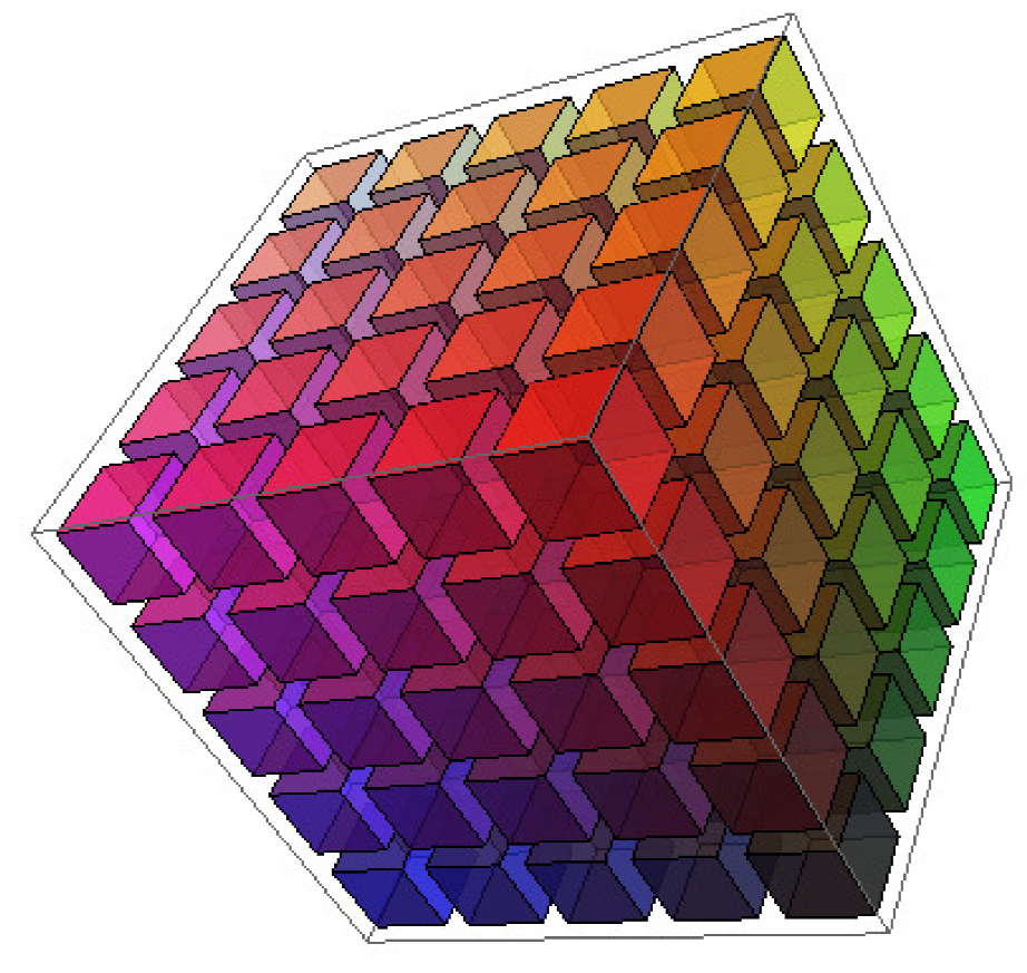
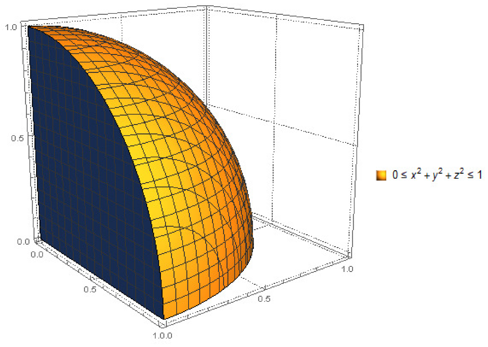
In this section, We present the graphical description of SLDFSs with reference or control parameters. We graphically examine that how its space is larger than the space of PFSs, SFSs, and T-SFSs. Figure 3, Figure 4 and Figure 5 gives us the geometrical representation of PiFS, SFS and SLDFS. Figure 6, Figure 7, Figure 8, Figure 9 and Figure 10 shows the grap of PiFS, SFS, T-SFS with some values of “n” and SLDFS.
It can be observed form Figure 10 and the graph of three grades/indexes in SLDFS provides a larger space than PiFS, SFS, and T-SFS. The addition of reference parameters provide freedom to the decision makers in selecting three grades/indexes. Thus a SLDFS with addition of reference parameter provides a robust approach for modeling uncertainties.
Operations on Spherical Linear Diophantine Fuzzy Numbers (SLDFNs)
In this subsection, we define some operations on SLDFNs. For the comparison of SLDFNs, we develop various score functions and accuracy functions.
Definition 9.
Let us consider for (indexing set) be an assembling of SLDFNs over the reference set and then the fundamental operations on SLDNFNs are the following
- ,
- ,
- ,
- ,
- ,
- ,
- ,
- ,
- .
Proposition 1.
Let and be two SLDFNs and , then and are also SLDFNs.
Proof.
The proof follows by using Definition 9. □
Example 1.
Let and be two SLDFNs, then
- Clearly by using Definition 9
If then
Proposition 2.
For two SLDFNs and with then and are also SLDFNs.
Proof.
Proof follows by using Definition 9. □
Chen and Tan [42] invented the idea of score functions for IFSs. Before that Tversky and Kahneman [43] proposed the same concept. We extend this idea for hybrid structures and SLDFNs. We invented different mappings to calculate the scores due to different strategies of approximation operators used in the proposed algorithms. These different score and accuracy functions determine the behavior of SLDFNs and provide us an appropriate optimal decision.
Definition 10.
Let be a SLDFN, then the mapping define a score function (SF) on scripted as
where is an assembling of SLDFNs over .
Definition 11.
The mapping defines an accuracy function (AF) scripted as
Definition 12.
The mapping defines a quadratic score function (QSF) for SLDFN defined as
Definition 13.
The mapping expresses the quadratic accuracy function (QAF) for SLDFN scripted as
Definition 14.
The expectation score function (ESF) on and scripted by the mapping such that
This is modified form of SF.
Definition 15.
Let and be SLDFNs. The binary relation on can be expressed as .
Definition 16.
Let and be SLDFNs. The binary relation on can be expressed as .
5. Spherical Linear Diophantine Fuzzy Soft Rough Sets (SLDFSRSs)
Definition 17.
Let be any set of objects, be the set of attributes, and take . A spherical linear Diophantine fuzzy soft set (SLDFSS) can be expressed by the mapping
where is an assembling of all SLDF-subsets of . A SLDFSS can be expressed as
Definition 18.
Let be a SLDFSS in . Then a SLDF-subset of is called spherical linear Diophantine fuzzy soft relation (SLDFSR) from to scripted as
where are satisfaction, uncertainty or abstinence and dissatisfaction grades respectively, with the corresponding reference parameters satisfying the constraints
If and , then SLDFSR on can be represented in tabular form as Table 4.
Definition 19.
For the reference set and set of decision variables , if we define a SLDFSR over , then is called a spherical linear Diophantine fuzzy soft approximation space (SLDFS-approximation space). If , then and are called upper and lower approximations of about respectively and scripted as
where
The pair is called SLDFSRS in . The lower and upper approximation operators are represented as and , respectively. If , then is said to be definable.
Example 2.
Let be the set of some famous shoe brands and be the collection of some attributes, where
We consider the SLDFSR, given by Table 5.
Consider a SLDF-subset of given as
By using Definition 19, we find the upper and lower approximations of given by
Now we can find other approximations of as follows.
Thus is called SLDFSRS.
Theorem 1.
For arbitrary , the upper and lower approximation operators and on SLDFS-approximation space satisfy the following axioms:
- (1)
- ,
- (2)
- ,
- (3)
- ,
- (4)
- ,
- (5)
- ,
- (6)
- ,
- (7)
- ,
- (8)
- .
The complement of is represented by .
Proof.
(1) From Definition 19
(2) We can prove this by Definition 19.
(3) By Definition 19, we consider that
(4) By following the Definition 19, we can write that
Thus .
The other axioms follows similar way. □
Proposition 3.
For arbitrary , the upper and lower approximation operators and on SLDFS-approximation space satisfy the following axioms:
- (1)
- ,
- (2)
- ,
- (3)
- ,
- (4)
- ,
- (5)
- ,
- (6)
- ,
- (7)
- ,
- (8)
- .
Proof.
Proof is obvious. □
Theorem 2.
For SLDFS-approximation space , if is serial, then and satisfy the following:
- (1)
- ,
- (2)
- .
Proof.
Proof is obvious by following Definition 19. □
Definition 20.
Let and let are lower and upper SLDFSR-approximation operators. Then ring sum operation of and is scripted as
6. Application of SLDFSRSs towards the Selection of Appropriate Clean Energy Technology
Ocean energy, biomass energy, wind energy, geothermal energy, and hydropower energy are all examples of clean energy technologies. These innovations are massive and are used to provide energy to the entire globe. In this section, we present an application that uses SLDFSRSs to select the most reliable and appropriate clean energy technology. We intended to develop two new algorithms.
6.1. Numerical Example
We suppose that a country wants to initiate an appropriate clean energy technology program for the development and to reach the industrial and social needs. They set a committee consisting on some energy and economical experts to construct a list of some clean energy technologies systems. The board of committee construct the set of feasible elements given as , where
Let be the set of attributes or decision parameters, where
The sub-criterion for attributes can be further categorized as follows:
- “Environmental: pollutant emission, land requirement, requirement for waste disposal” means that the alternative is “friendly”, “average” or may be “not-friendly” for the environment.
- “Socio-political: Government policy, labor impact, social acceptance” means that the alternative has “maximum”, “average” or “minimum” acceptance.
- “Economic: implementation cost, economic value, affordability” means that the alternative is “expensive”, “affordable” or may be “cheap”.
- “Technological and quality of energy resource: continuity and predictability of the performance risk, local technical knowledge, sustainability, durability” means that the alternative is “highly”, “medium” or may be “low” technical.
The tabular representation of these sub-criteria can be seen in Table 6.
We proposed two new algorithms (Algorithms 1 and 2) by using SLDFSRSs for the selection of best clean energy technology. The graphical view of both algorithms is given in Figure 11.
| Algorithm 1 Selection of a best clean energy technology by using SLDFSRSs |
| Input: 1. Consider as an initial universe. 2. Consider as a set of attributes. Construction: 3. Executing the efficiency of DMs, build a SLDFSR . 4. Compute SLDF-subset of as an optimal normal decision set. Calculation: 5. Find the SLDFSR-approximation operators and as lower and upper approximations with the help of Definition 19. 6. Find the ring sum and the choice SLDFS. Output: 7. By using Definitions 10, 12, 14, calculate score, quadratic score and expectation score of every alternative in . 8. By using Definition 16, find the ranking of alternatives. Final decision: 9. An alternative with highest score function value is the required optimal alternative. |
| Algorithm 2 Selection of a best clean energy technology by using SLDFSRSs |
| Input: 1. Consider as a universe of discourse. 2. Consider as a set of attributes. Construction: 3. Executing the efficiency of DMs, construct a SLDFSR . 4. Find SLDF-subset of as an optimal normal decision set. Calculation: 5. Find the SLDFSR-approximation operators and as lower and upper approximations by using Definition 19. 6. For “” number of experts, estimate upper and lower reducts, respectively. Output: 7. Form calculated “” reducts, we get “” crisp subsets of the reference set . The subsets can be constructed by using the “YES” and “NO” logic. Then “YES” gives the optimal object. 8. Find the core by calculating the intersection of all reducts. Final decision: 9. An alternative with highest score function value is the required optimal alternative. |
6.1.1. Calculations by Algorithm 1
According to the environment of land and considering some important factors, the experts of committee give their preferences to the alternatives corresponding to the selected criteria. The verbal information can be converted into the SLDFNs by using linguistic term logic. The indiscernibility relation is “the selection of best clean energy technology”. This relation can be observed by SLDFSR, given as Table 7.
Thus be a SLDFSR on . This relation gives us the numeric values in the form of SLDFNs of each alternative corresponding to every decision variable. For example, for the alternative the decision variable (“Environmental: pollutant emission, land requirement, requirement for waste disposal”) has numeric value . This value shows that the alternative is suitable for the environment, is abstinence and is its falsity value. The triplet represents the reference parameters for the satisfaction, abstinence and dissatisfaction grades, where we can observe that alternative is friendly, average and is not friendly for environment.
The set is SLDF-subset of and scripted as follows
The lower and upper approximations of LDFS on LDFSR are as follows.
Now we calculate the score values, quadratic score values and expectation score values of alternatives in by using Definitions 10, 12 and 14. The calculated data with final ranking is given in Table 8.
6.1.2. Calculations by Algorithm 2
The initial 5 steps of Algorithm 1 are same as Algorithm 2. Now we compute the upper and lower reducts from upper and lower approximations of SLDFS. Consider a committee of three experts given as
The reducts from approximations can be constructed by using the following terms.
The final decision is based on the and given in Table 9
For expert-X, the upper reduct of upper approximation (calculated in Algorithm 1) of SLDFS is given as Table 10. The average of score values of all the alternatives for is .
This implies that . For expert-X, the lower reduct of lower approximation (calculated in Algorithm 1) of SLDFS is given as Table 11. The average of score values of all the alternatives for is .
This implies that . For expert-Y, the upper reduct of upper approximation (calculated in Algorithm 1) of SLDFS is given as Table 12.
This implies that . For expert-Y, the lower reduct of lower approximation (calculated in Algorithm 1) of SLDFS is given as Table 13.
This implies that . For expert-Z, the upper reduct of upper approximation (calculated in Algorithm 1) of SLDFS is given as Table 14.
This implies that . For expert-Z, the lower reduct of lower approximation (calculated in Algorithm 1) of SLDFS is given as Table 15.
This implies that . Now we calculate the core by taking the intersection of all upper and lower reducts for all three experts.
This means that “” (geothermal power plant) is the most suitable alternative for the final decision.
6.2. Advantages, Superiority, and Novelty of Proposed Algorithms
In this subsection, we discuss the advantages, superiority, and novelty of proposed algorithms.
- Proposed Algorithms 1 and 2 are designed to deal with real-life problems based on novel hybrid approach of spherical linear Diophantine fuzzy soft rough sets (SLDFSRSs) and to utilize the characteristics of existing models like soft sets, rough sets, and spherical linear Diophantine fuzzy sets. A hybrid model is always more efficient, powerful and reliable to deal with uncertain real-life problems. A hybrid model can be utilized to handle multiple issues, multiple criterion, and multiple paradigms.
- Algorithms 1 and 2 are developed to examine the role of reference parameters in spherical linear Diophantine fuzzy sets. The existing algorithms based on PFSs, SFSs, T-SFSs, and neutrosophic sets cannot deal with parameterizations. The proposed algorithm provide freedom to the decision-maker(DM) to select grades/indexes without any restriction. The dynamic features of reference parameters can classify and effectively resolve uncertain multi-criteria decision-making (MCDM) problems.
- The proposed approach is efficient and suitable for any kind of uncertain information. The space of existing theories such as PFSs, SFSs, T-SFSs, and neutrosophic sets can be enhanced by proposed model of spherical linear Diophantine fuzzy sets. This model increases the valuation space of three (satisfaction, abstinence, and dissatisfaction) indexes/degrees. The algorithms are simple to understand, easy to apply, and efficient on diverse kinds of alternatives and attributes.
- Various score functions has been established by Feng et al. [66] for IFSs. We developed three different kinds of score functions named as “score function” (SF), “quadratic score function” (QSF), and “expectation score function” (ESF). We also establish their associated accuracy functions to compare the SLDFNs. The slight difference in ordering of optimal results is due to diverse strategies of score functions in the calculations. Table 8 implies the difference in ordering for the worst alternatives. Although it is fascinating to examine that final result from both algorithms are equivalent for all varieties of score functions.
6.3. Comparison Analysis
The comparison of proposed model SLDFSRSs and Algorithms 1 and 2 with some existing models and algorithms is given to discuss advantage, superiority, and validity of proposed approach. Table 16 represents the characteristics of suggested SLDFSRSs and ranking of alternatives computed by different techniques.
For two proposed algorithms based on SLDFSRSs and its SLDFS-approximation spaces, the final results for the decision-making problem of clean energy technique selection is given in Table 17.
The optimal alternative computed by the both algorithms is exactly same. Hence the alternative (geothermal power plant) is the optimal selected alternative.
7. Conclusions
We studied certain fuzzy sets including PiFSs, SFSs, T-SFSs, and NSs. These extension have a large number of applications in solving real-life problems, and many researchers have been successfully applied these extensions. Unfortunately, these extensions have some strict limitations on indexes/grades. In order to deal with such problems, we introduced a robust hybrid model named as spherical linear diophantine fuzzy set which fusion of spherical linear Diophantine fuzzy set (SLDFS), soft set, and rough set. The addition of reference parameters in SLDFS provide freedom to the decision makers (DMs) for the selection of indexes/grades. A SLDFS is an efficient model to deal with uncertainties due to addition of reference parameters and . We presented the graphical representation of SLDFS to compare it with some existing extensions of fuzzy sets. We introduced various score functions and accuracy functions to compare SLDFNs. We prolonged the idea of SLDFSs to SLDFSRSs by joining SLDFSs, rough sets, and soft sets. We investigated some new results for upper and lower approximation operators of SLDFSRSs. We developed two new algorithms for multi-criteria decision making (MCDM) based on SLDFSRSs. We presented a brief association among the recommended and existing theories and examined the strong impact of proposed structures to the MCDM problems. To resolve the real-world problems these findings will be fruitful and supportive for the scholars and decision-makers. In future, we will investigate the real-life problems associated with the ideas based on SLDF-graphs, SLDF-topology, and SLDF-information measures.
Author Contributions
M.R.H., S.T.T., M.R., D.P. and G.C., originated the research plan and started to work together to write this manuscript, M.R., G.C. and D.P., developed the algorithms for data analysis and design the model of the manuscript, M.R.H., S.T.T. and D.P., processed the data collection and wrote the paper. All authors have read and agreed to the published version of the manuscript.
Funding
This research received no external funding.
Institutional Review Board Statement
Not applicable.
Informed Consent Statement
Not applicable.
Data Availability Statement
Not applicable.
Conflicts of Interest
The authors declare no conflict of interest.
References
- Zadeh, L.A. Fuzzy sets. Inf. Control 1965, 8, 338–353. [Google Scholar] [CrossRef] [Green Version]
- Zadeh, L.A. The concept of a linguistic variable and its application to approximate reasoning—I. Inf. Sci. 1975, 8, 199–249. [Google Scholar] [CrossRef]
- Atanassov, K.T. Intuitionistic fuzzy sets. In VII ITKRs Session; Sgurev, V., Ed.; Central Sci. and Techn. Library, Bulg. Academy of Sciences: Sofia, Bulgaria, 1984; reprinted in Int. J. Bioautom. 2016, 20, S1–S6. [Google Scholar]
- Atanassov, K.T.; Stoeva, S. Intuitionistic fuzzy sets. In Proceedings of the Polish Symposium on Interval and Fuzzy Mathematics, Poznan, Poland, 23–26 August 1983. [Google Scholar]
- Atanassov, K.T. Intuitionistic fuzzy sets. Fuzzy Sets Syst. 1986, 20, 87–96. [Google Scholar] [CrossRef]
- Atanassov, K.T. Geometrical interpretation of the elemets of the intuitionistic fuzzy objects. Int. J. Bio-Autom. 2016, 20 (Suppl. 1), S27–S42. [Google Scholar]
- Yager, R.P. Pythagorean fuzzy subsets. In Proceedings of the IFSA World Congress and NAFIPS Annual Meeting, Edmonton, AB, Canada, 24–28 June 2013; pp. 57–61. [Google Scholar]
- Yager, R.P. Pythagorean membership grades in multi criteria decision-making. IEEE Trans. Fuzzy Syst. 2014, 22, 958–965. [Google Scholar] [CrossRef]
- Yager, R.P. Generalized orthopair fuzzy sets. IEEE Trans. Fuzzy Syst. 2017, 25, 1222–1230. [Google Scholar] [CrossRef]
- Smarandache, F. A Unifying Field in Logics: Neutrosophic Logic. Neutrosophy, Neutrosophic Set, Neutrosophic Probability and Statistics, 5th ed.; American Research Press: Rehoboth, DE, USA, 2006; pp. 1–155. [Google Scholar]
- Cuong, B.C. Picture fuzzy sets-first results. In Preprint of Seminar on Neuro-Fuzzy Systems with Applications; Institute of Mathematics: Hanoi, Vietnam, May 2013; Part 1. [Google Scholar]
- Cuong, B.C. Picture fuzzy sets-first results. In Preprint of Seminar on Neuro-Fuzzy Systems with Applications; Institute of Mathematics: Hanoi, Vietnam, June 2013; Part 2. [Google Scholar]
- Cuong, B.C.; Kreinovich, V. Picture fuzzy sets—A new concept for computational intelligence problems. In Proceedings of the 3rd World Congress on Information and Communication Technologies (WICT), Hanoi, Vietnam, 15–18 December 2013. [Google Scholar]
- Mahmood, T.; Ullah, K.; Khan, Q.; Jan, N. An approach toward decision-making and medical diagnosis problems using the concept of spherical fuzzy sets. Neural Comput. Appl. 2019, 31, 7041–7053. [Google Scholar] [CrossRef]
- Mahmood, T.; Mehmood, F.; Khan, Q. Some generalized aggregation operators for cubic hesitant fuzzy sets and their application to multi criteria decision making. Punjab Univ. J. Math. 2017, 49, 31–49. [Google Scholar]
- Suapang, P.; Dejhan, K.; Yimmun, S. Medical image processing and analysis for nuclear medicine diagnosis. In Proceedings of the International Conference on Control Automation and Systems (ICCAS), Gyeonggi-do, Korea, 27–30 October 2010. [Google Scholar] [CrossRef]
- Akbarizadeh, G.; Moghaddam, A.E. Detection of lung nodes in CT scans based on unsupervised feature learning and fuzzy inference. J. Med Imaging Health Inform. 2016, 6, 477–483. [Google Scholar] [CrossRef]
- Akbarizadeh, G. A new statistical-based kurtosis wavelet energy feature for texture recognition of SAR images. IEEE Trans. Geosci. Remote Sens. 2012, 50, 4358–4368. [Google Scholar] [CrossRef]
- Akbarizadeh, G. Segmentation of SAR satellite images unsing cellular learning automata and adaptive chains. J. Remote Sens. Technol. 2013, 1, 44. [Google Scholar] [CrossRef]
- Akbarizadeh, G.; Rahmani, M. A new ensemble clustering method for PolSAR image segmentation. In Proceedings of the 7th Conference on Information Knowledge and Technology (IKT), Urmia, Iran, 26–28 May 2015. A New Computer Vision Algorithm for Classification of POLSAR Images. [Google Scholar] [CrossRef]
- Akbarizadeh, G.; Tirandaz, Z.; Kooshesh, M. A new curvelet-based texture classification approach for land cover recognition of SAR satellite images. Malays. J. Comput. Sci. 2014, 27, 218–239. [Google Scholar]
- Akbarizadeh, G.; Tirandaz, Z. Segmentation parameter estimation algorithm based on curvelet transform coefficients energy for feature extraction and texture description of SAR images. In Proceedings of the 7th Conference on Information and Knowledge Technology (IKT), Urmia, Iran, 26–28 May 2015. [Google Scholar] [CrossRef]
- Akbarizadeh, G.; Rahmani, M. Efficient combination of texture and color features in a new spectral clustering method for PolSAR image segmentation. Natl. Acad. Sci. Lett. 2017, 40, 117–120. [Google Scholar] [CrossRef]
- Benz, U.C.; Hofmann, P.; Willhauck, G.; Lingenfelder, I.; Heynen, M. Multi-resolution object-oriented fuzzy analysis of remote sensing data for GIS-ready information. ISPRS J. Photogramm. Remote Sens. 2004, 58, 239–258. [Google Scholar] [CrossRef]
- Gong, M.; Zhou, Z.; Ma, J. Change detection in synthetic aperture redar images based on image fusion and fuzzy clustering. IEEE Trans. Image Process. 2012, 21, 2141–2151. [Google Scholar] [CrossRef]
- Modava, M.; Akbarizadeh, G. Coastline extraction from SAR images using spatial fuzzy clustering and the active contour method. Int. J. Remote Sens. 2017, 38, 355–370. [Google Scholar] [CrossRef]
- Modava, M.; Akbarizadeh, G. A level set based method for coastline detection of SAR images. In Proceedings of the 3rd International Conference on Patteren Recognition and Image Analysis (IPRIA), Shahrekord, Iran, 19–20 April 2017. [Google Scholar] [CrossRef]
- Shanmugan, K.S.; Narayanan, V.; Frost, V.S.; Stiles, J.A.; Holtzman, J.C. Textural features for redar image analysis. IEEE Trans. Geosci. Remote Sens. 1981, 3, 153–156. [Google Scholar] [CrossRef]
- Tirandaz, Z.; Akbarizadeh, G. A two-phased algorithm based on kurtosis curvelet energy and unsupervised spectral regression for segmentation for SAR images. IEEE J. Sel. Top. Appl. Earth Obs. Remote Sens. 2016, 9, 1244–1264. [Google Scholar] [CrossRef]
- Ahmadi, N.; Akbarizadeh, G. Hybrid robust iris recognition approach using iris image pre-processing, two-dimensional gabor features and multi-layer perceptron neural network/PSO. IET Biom. 2018, 7, 153–162. [Google Scholar] [CrossRef]
- Duagman, J. How iris recognition works. In The Essential Guide to Image Processing; Academic Press: Cambridge, MA, USA, 2009; pp. 715–739. [Google Scholar] [CrossRef]
- Andekah, Z.A.; Naderan, M.; Akbarizadeh, G. Semi-supervised Hyperspectral image classification using spatial-spectral features and superpixel-based sparse codes. In Proceedings of the Iranian Conference of Electrical Engineering (ICEE), Tehran, Iran, 2–4 May 2017. [Google Scholar] [CrossRef]
- Perić, N. Fuzzy logic and fuzzy set theory based edge detection algorithm. Serbian J. Electr. Eng. 2015, 12, 109–116. [Google Scholar] [CrossRef] [Green Version]
- Molodtsov, D. Soft set theory-first results. Comput. Math. Appl. 1999, 37, 19–31. [Google Scholar] [CrossRef] [Green Version]
- Maji, P.K.; Biswas, R.; Roy, A.R. Soft set theory. Comput. Math. Appl. 2003, 45, 555–562. [Google Scholar] [CrossRef] [Green Version]
- Pawlak, Z. Rough sets. Int. J. Comput. Inf. Sci. 1982, 2, 145–172. [Google Scholar] [CrossRef]
- Pawlak, Z.; Skowron, A. Rough sets: Some extensions. Inf. Sci. 2007, 177, 28–40. [Google Scholar] [CrossRef] [Green Version]
- Ali, M.I. Another view on q-rung orthopair fuzzy sets. Int. J. Intell. Syst. 2018, 33, 2139–2153. [Google Scholar] [CrossRef]
- Ali, M.I.; Shabir, M. Logic connectives for soft sets and fuzzy soft sets. IEEE Trans. Fuzzy Syst. 2014, 22, 1431–1442. [Google Scholar] [CrossRef]
- Agarwal, M.; Biswas, K.K.; Hanmandlu, M. Generalized intuitionitic fuzzy soft sets with applications in decision-making. Appl. Soft Comput. 2013, 20, 3552–3566. [Google Scholar] [CrossRef]
- Garg, H. A new generalized Pythagorean fuzzy information aggregation using Einstein operations and its application to decision making. Int. J. Intell. Syst. 2016, 31, 886–920. [Google Scholar] [CrossRef]
- Chen, S.M.; Tan, M.J. Handling multi-criteria fuzzy decision-makling problems based on vague set theory. Fuzzy Sets Syst. 1994, 67, 163–172. [Google Scholar] [CrossRef]
- Tversky, A.; Kahneman, D. Advances in prospect theory: Cumulative representation of uncertainity. J. Risk Uncertain. 1992, 5, 297–323. [Google Scholar] [CrossRef]
- Jose, S.; Kuriaskose, S. Aggregation operators, score function and accuracy function for multi criteria decision making in intuitionistic fuzzy context. Notes Intuitionist Fuzzy Sets 2014, 20, 40–44. [Google Scholar]
- Wang, H.; Smarandache, F.; Zhang, Y.Q.; Sunderraman, R. Single valued neutrosophic sets. Multispace Multistruct. 2010, 4, 410–413. [Google Scholar]
- Peng, X.; Yang, Y. Some results for pythagorean fuzzy sets. Int. J. Intell. Syst. 2015, 30, 1133–1160. [Google Scholar] [CrossRef]
- Peng, X.; Garg, H. Algorithms for interval-valued fuzzy soft sets in emergency decision-making based on WDBA and CODAS with new information measure. Comput. Ind. Eng. 2018, 119, 439–452. [Google Scholar] [CrossRef]
- Xu, Z.S. Intuitionistic fuzzy aggregation operators. IEEE Trans. Fuzzy Syst. 2007, 15, 1179–1187. [Google Scholar]
- Xu, Z.; Cai, X. Intuitionistic Fuzzy Information Aggregation: Theory and Applications; Science Press: Beijing, China; Springer: Berlin/Heidelberg, Germany, 2012. [Google Scholar]
- Xu, Z. Studies in Fuzziness and Soft Computing: Hesitant Fuzzy Sets Theory; Springer International Publishing: Cham, Switzerland, 2014. [Google Scholar]
- Ye, J. Linguistic neutrosophic cubic numbers and their multiple attribute decision-making method. Information 2017, 8, 110. [Google Scholar] [CrossRef] [Green Version]
- Jana, C.; Senapati, T.; Pal, M.; Yager, R.R. Picture fuzzy Dombi aggreegation operators: Application to MADM process. Appl. Soft Comput. J. 2019, 74, 99–109. [Google Scholar] [CrossRef]
- Xu, Y.; Shang, X.; Wang, J.; Zhang, R.; Li, W.; Xing, Y. A method to multi-attribute decision-making with picture fuzzy information based on Muirhead mean. J. Intell. Fuzzy Syst. 2018, 36, 1–17. [Google Scholar] [CrossRef]
- Wang, R.; Wang, J.; Gao, H.; Wei, G. Methods for MADM with picture fuzzy Muirhead mean operators and their applications for evaluating the financial investment risk. Symmetry 2019, 11, 6. [Google Scholar] [CrossRef] [Green Version]
- Wang, R.; Li, Y. Picture hesitant fuzzy set and its applications to multiple criteria decision-making. Symmetry 2018, 10, 295. [Google Scholar] [CrossRef] [Green Version]
- Khan, S.; Abdullah, S.; Abdullah, L.; Ashraf, S. Logarithmic aggregation operators of picture fuzzy numbers for multi-attribute decision-making problems. Mathematics 2019, 7, 608. [Google Scholar] [CrossRef] [Green Version]
- Khan, S.; Abdullah, S.; Ashraf, S. Picture fuzzy aggregation information based on Einstein operations and their application in decision-making. Math. Sci. 2019, 13, 213–229. [Google Scholar] [CrossRef] [Green Version]
- Zhang, L.; Zhan, J.; Xu, Z.X. Covering-based generalized IF rough sets with applications to multi-attribute decision-making. Inf. Sci. 2019, 478, 275–302. [Google Scholar] [CrossRef]
- Zhang, H.; Shu, L.; Liao, S. Intuitionistic fuzzy soft rough set and its applications in decision-making. Abstr. Appl. Anal. 2014, 2014, 287314. [Google Scholar] [CrossRef] [Green Version]
- Zhang, H.; Dong, Y.; Carrascosa, I.P.; Zhou, H. Failure mode and effect analysis in a linguistic context: A consensus-based multi-attribute group decision-making approach. IEEE Trans. Reliab. 2019, 68, 566–582. [Google Scholar] [CrossRef] [Green Version]
- Zhang, H.; Zhang, R.; Huang, H.; Wang, J. Some picture fuzzy Dombi Heronian mean operators with their applications to multi-attribute decision-making. Symmetry 2018, 10, 593. [Google Scholar] [CrossRef] [Green Version]
- Zhang, Z.; Kou, X.; Yu, W.; Guo, C. On priority weights and consistency for incomplete hesitant fuzzy preference relations. Knowl. Based Syst. 2018, 143, 115–126. [Google Scholar] [CrossRef]
- Zhang, Z.; Guo, C. Deriving priority weights from intuitionistic multiplicative preference relations under group decision-making settings. J. Oper. Res. Soc. 2017, 68, 1582–1599. [Google Scholar] [CrossRef]
- Zhang, Z.; Guo, C.; Martine, L. Managing multigranular linguistic distribution assessments in large-scale multiattribute group decision-making. IEEE Trans. Syst. Man Cybern. Syst. 2017, 47, 3063–3076. [Google Scholar] [CrossRef] [Green Version]
- Zhang, B.; Dong, Y.; Viedma, E.H. Group decision making with heterogeneous preference structures: An automatic mechanism to support consensus reaching. Nigotiation 2019, 28, 585–617. [Google Scholar] [CrossRef]
- Feng, F.; Fujita, H.; Ali, M.I.; Yager, R.R.; Liu, X. Another view on generalized intuitionistic fuzzy soft sets and related multi-attribute decision making methods. IEEE Trans. Fuzzy Syst. 2019, 27, 474–488. [Google Scholar] [CrossRef]
- Guo, K. Amount of information and attitudinal-based method for ranking Atanassov’s intuitionistic fuzzy values. IEEE Trans. Fuzzy Syst. 2014, 22, 177–188. [Google Scholar] [CrossRef]
- Liu, P.; Wang, P. Some q-rung orthopair fuzzy aggregation operators and their applications to multiple-attribute decision-making. Int. J. Intell. Syst. 1983, 33, 259–280. [Google Scholar] [CrossRef]
- Riaz, M.; Hashmi, M.R. Linear Diophantine fuzzy set and its applications towards multi-attribute decision making problems. J. Intell. Fuzzy Syst. 2019, 37, 5417–5439. [Google Scholar] [CrossRef]
- Riaz, M.; Hashmi, M.R. Soft rough Pythagorean m-polar fuzzy sets and Pythagorean m-polar fuzzy soft rough sets with application to decision-making. Comput. Appl. Math. 2020, 39, 1–36. [Google Scholar] [CrossRef]
- Riaz, M.; Pamucar, D.; Farid, H.M.A.; Hashmi, M.R. q-Rung orthopair fuzzy prioritized aggregation operators and their application towards green supplier chain management. Symmetry 2020, 12, 976. [Google Scholar] [CrossRef]
- Vashist, R. An algorithm for finding the reduct and core of the consistent dataset. In Proceedings of the International Conference on Computational Intelligence and Communications Networks, Jabalpur, India, 12–14 December 2015. [Google Scholar] [CrossRef]
- Wang, C.; Zhou, X.; Tu, H.; Tao, S. Some geometric aggregation operators based on picture fuzzy sets and their applications in multiple-attribute decision-making. Iran. J. Pure Appl. Math. 2017, 37, 477–492. [Google Scholar]
- Zhan, J.; Alcantud, J.C.R. A novel type of soft rough covering and its application to multi-criteria group decision-making. Artif. Intell. Rev. 2018, 52, 2381–2410. [Google Scholar] [CrossRef]
- Riaz, M.; Çagman, N.; Wali, N.; Mushtaq, A. Certain properties of soft multi-set topology with applications in multi-criteria decision making. Decis. Mak. Appl. Manag. Eng. 2020, 3, 70–96. [Google Scholar] [CrossRef]
- Sahu, R.; Dash, S.R.; Das, S. Career selection of students using hybridized distance measure based on picture fuzzy set and rough set theory. Decis. Mak. Appl. Manag. Eng. 2021, 4, 104–126. [Google Scholar] [CrossRef]
- Ali, Z.; Mahmood, T.; Ullah, K.; Khan, Q. Einstein Geometric Aggregation Operators using a Novel Complex Interval-valued Pythagorean Fuzzy Setting with Application in Green Supplier Chain Management. Rep. Mech. Eng. 2021, 2, 105–134. [Google Scholar] [CrossRef]
- Alosta, A.; Elmansuri, O.; Badi, I. Resolving a location selection problem by means of an integrated AHP-RAFSI approach. Rep. Mech. Eng. 2021, 2, 135–142. [Google Scholar] [CrossRef]
- Yorulmaz, Ö; Kuzu Yildirim, S.; Yildirim, B.F. Robust Mahalanobis Distance based TOPSIS to Evaluate the Economic Development of Provinces. Oper. Res. Eng. Sci. Theory Appl. 2021, 4, 102–123. [Google Scholar] [CrossRef]
- Pamucar, D.; Ecer, F. Prioritizing the weights of the evaluation criteria under fuzziness: The fuzzy full consistency method—FUCOM-F. Facta Univ. Ser. Mech. Eng. 2020, 18, 419–437. [Google Scholar] [CrossRef]
- Ramakrishnan, K.R.; Chakraborty, S. A cloud TOPSIS model for green supplier selection. Facta Univ. Ser. Mech. Eng. 2020, 18, 375–397. [Google Scholar]
- Kishore, R.; Mousavi Dehmourdi, S.A.; Naik, M.G.; Hassanpour, M. Designing a framework for Subcontractor’s selection in construction projects using MCDM model. Oper. Res. Eng. Sci. Theory Appl. 2020, 3, 48–64. [Google Scholar] [CrossRef]
- Zararsiz, Z. Similarity measures of sequence of fuzzy numbers and fuzzy risk analysis. Adv. Math. Phys. 2015, 2015, 724647. [Google Scholar] [CrossRef] [Green Version]
- Zararsiz, Z. Measuring entropy values of QRS-complexes before and after training program of sport horses with ECG. Ann. Fuzzy Math. Inform. 2018, 15, 243–251. [Google Scholar] [CrossRef]
Figure 1.
Graph of satisfaction and dissatisfaction grades of IFS.

Figure 2.
Graph of satisfaction, abstinence, and dissatisfaction grades of SLDFS.

Figure 3.
Graph of three indexes of PiFS.

Figure 4.
Graph of three indexes of SFS.

Figure 5.
Graph of three indexes of SLDFS.

Figure 6.
Graph of three indexes of PFS.

Figure 7.
Graph of three indexes of SFS.

Figure 8.
Graph of three indexes of T-SFS with n = 5.

Figure 9.
Graph of three indexes of T-SFS with n = 100.

Figure 10.
Graph of three indexes of SLDFS for reference parameters .

Figure 11.
Flow chart diagram of Algorithms 1 and 2.

Figure 12.
Bar chart of alternatives under SLDFSRS for SF (), QSF () and ESF ().


Table 1.
SLDFS.
Table 2.
SLDFS.
Table 3.
SLDFS.
Table 4.
Spherical linear Diophantine fuzzy soft relation (SLDFSR).
| … | |||
|---|---|---|---|
| … | |||
| … | |||
| … |
Table 5.
SLDFSR.
| Numeric Values of SLDFNs | |
|---|---|
| : | |
| : | |
| : | |
| : | |
| : | |
| : |
Table 6.
Characteristics of selected decision variables.
| Decision Variables | Characteristics for SLDFSR |
|---|---|
| Environmental: land requirement, pollutant emission, requirement for waste disposal | |
| Socio-political: Government policy, social acceptance, labor impact | |
| Economic: implementation cost, economic value, affordability | |
| Technological and quality of energy resource: continuity and predictability of the performance risk, sustainability, local technical knowledge, durability |
Table 7.
SLDFSR.
| SLDFNs | SLDFNs | |
|---|---|---|
Table 8.
Ranking of alternatives for different score values.
| LDFS | Ranking | Rank Orders | Final Decision | ||||||
|---|---|---|---|---|---|---|---|---|---|
| (SF) | |||||||||
| (QSF) | |||||||||
| (ESF) |
Table 9.
The criteria for the final decision (F.D).
| F.D | ||
|---|---|---|
| 0 | NO | NO |
| 1 | YES | YES |
| 0 | YES | NO |
| 1 | NO | NO |
Table 10.
Upper reduct for expert-X from .
| F.D | ||||||||||
|---|---|---|---|---|---|---|---|---|---|---|
| 1 | YES | YES | ||||||||
| 0 | NO | NO | ||||||||
| 1 | NO | NO | ||||||||
| 0 | NO | NO | ||||||||
| 1 | YES | YES | ||||||||
| 1 | YES | YES |
Table 11.
Lower reduct for expert-X from .
| F.D | ||||||||||
|---|---|---|---|---|---|---|---|---|---|---|
| 1 | NO | NO | ||||||||
| 0 | NO | NO | ||||||||
| 1 | YES | YES | ||||||||
| 0 | YES | NO | ||||||||
| 1 | YES | YES | ||||||||
| 1 | NO | NO |
Table 12.
Upper reduct for expert-Y from .
| F.D | ||||||||||
|---|---|---|---|---|---|---|---|---|---|---|
| 0 | YES | NO | ||||||||
| 1 | NO | NO | ||||||||
| 0 | NO | NO | ||||||||
| 1 | NO | NO | ||||||||
| 1 | YES | YES | ||||||||
| 1 | YES | YES |
Table 13.
Lower reduct for expert-Y from .
| F.D | ||||||||||
|---|---|---|---|---|---|---|---|---|---|---|
| 0 | NO | NO | ||||||||
| 1 | NO | NO | ||||||||
| 0 | YES | NO | ||||||||
| 1 | YES | YES | ||||||||
| 1 | YES | YES | ||||||||
| 1 | NO | NO |
Table 14.
Upper reduct for expert-Z from .
| F.D | ||||||||||
|---|---|---|---|---|---|---|---|---|---|---|
| 1 | YES | YES | ||||||||
| 0 | NO | NO | ||||||||
| 1 | NO | NO | ||||||||
| 1 | NO | NO | ||||||||
| 1 | YES | YES | ||||||||
| 0 | YES | NO |
Table 15.
Lower reduct for expert-Z from .
| F.D | ||||||||||
|---|---|---|---|---|---|---|---|---|---|---|
| 1 | NO | NO | ||||||||
| 0 | NO | NO | ||||||||
| 1 | YES | YES | ||||||||
| 1 | YES | YES | ||||||||
| 1 | YES | YES | ||||||||
| 0 | NO | NO |
Table 16.
Comparison analysis of proposed concepts with existing ideas.
| Concepts | Satisfaction Grade | Abstinence Grade | Dissatisfaction Grade | Refusal Grade |
|---|---|---|---|---|
| Fuzzy set [1] | ✓ | × | × | × |
| Neutrosophic set [10] | ✓ | ✓ | ✓ | × |
| Rough set [36] | × | × | × | × |
| Soft set [34] | × | × | × | × |
| Picture fuzzy set [11,12,13] | ✓ | ✓ | ✓ | ✓ |
| Spherical fuzzy set [14] | ✓ | ✓ | ✓ | ✓ |
| T-spherical fuzzy set [14] | ✓ | ✓ | ✓ | ✓ |
| LDFS [69] | ✓ | ✓ | ✓ | × |
| SLDFS (proposed) | ✓ | ✓ | ✓ | ✓ |
| SLDFSS (proposed) | ✓ | ✓ | ✓ | ✓ |
| SLDFSRS (proposed) | ✓ | ✓ | ✓ | ✓ |
| Concepts | Reference Parameterizations | Upper and Lower Approximations | Boundary Region | Multi-Valued Parameterizations |
| Fuzzy set [1] | × | × | × | × |
| Neutrosophic set [10] | × | × | × | × |
| Rough set [36] | × | ✓ | ✓ | × |
| Soft set [34] | × | × | × | ✓ |
| Picture fuzzy set [11,12,13] | × | × | × | × |
| Spherical fuzzy set [14] | × | × | × | × |
| T-spherical fuzzy set [14] | × | × | × | × |
| LDFS [69] | ✓ | × | × | × |
| SLDFS (proposed) | ✓ | × | × | × |
| SLDFSS (proposed) | ✓ | × | × | ✓ |
| SLDFSRS (proposed) | ✓ | ✓ | ✓ | ✓ |
Table 17.
Comparison of results obtained from proposed algorithms.
| Proposed Algorithm | Score Function | Core | Optimal Decision |
|---|---|---|---|
| Algorithm 1 | × | ||
| Algorithm 1 | × | ||
| Algorithm 1 | × | ||
| Algorithm 2 | × | ✓ |
Publisher’s Note: MDPI stays neutral with regard to jurisdictional claims in published maps and institutional affiliations. |
© 2021 by the authors. Licensee MDPI, Basel, Switzerland. This article is an open access article distributed under the terms and conditions of the Creative Commons Attribution (CC BY) license (https://creativecommons.org/licenses/by/4.0/).
Share and Cite
MDPI and ACS Style
Hashmi, M.R.; Tehrim, S.T.; Riaz, M.; Pamucar, D.; Cirovic, G. Spherical Linear Diophantine Fuzzy Soft Rough Sets with Multi-Criteria Decision Making. Axioms 2021, 10, 185. https://0-doi-org.brum.beds.ac.uk/10.3390/axioms10030185
AMA Style
Hashmi MR, Tehrim ST, Riaz M, Pamucar D, Cirovic G. Spherical Linear Diophantine Fuzzy Soft Rough Sets with Multi-Criteria Decision Making. Axioms. 2021; 10(3):185. https://0-doi-org.brum.beds.ac.uk/10.3390/axioms10030185
Chicago/Turabian StyleHashmi, Masooma Raza, Syeda Tayyba Tehrim, Muhammad Riaz, Dragan Pamucar, and Goran Cirovic. 2021. "Spherical Linear Diophantine Fuzzy Soft Rough Sets with Multi-Criteria Decision Making" Axioms 10, no. 3: 185. https://0-doi-org.brum.beds.ac.uk/10.3390/axioms10030185
Note that from the first issue of 2016, this journal uses article numbers instead of page numbers. See further details here.