The Approximate and Analytic Solutions of the Time-Fractional Intermediate Diffusion Wave Equation Associated with the Fokker–Planck Operator and Applications

Abstract

In this paper, the time-fractional wave equation associated with the space-fractional Fokker–Planck operator and with the time-fractional-damped term is studied. The concept of the Green function is implemented to drive the analytic solution of the three-term time-fractional equation. The explicit expressions for the Green function $G_3\left(t\right)$ of the three-term time-fractional wave equation with constant coefficients is also studied for two physical and biological models. The explicit analytic solutions, for the two studied models, are expressed in terms of the Weber, hypergeometric, exponential, and Mittag–Leffler functions. The relation to the diffusion equation is given. The asymptotic behaviors of the Mittag–Leffler function, the hypergeometric function $1F1$, and the exponential functions are compared numerically. The Grünwald–Letnikov scheme is used to derive the approximate difference schemes of the Caputo time-fractional operator and the Feller–Riesz space-fractional operator. The explicit difference scheme is numerically studied, and the simulations of the approximate solutions are plotted for different values of the fractional orders.

1. Introduction and Important Definitions

The classical intermediate diffusion wave equation, the multiterm wave equation, can be written as:

$$\frac{{\partial }^{2}u(x,t)}{\partial t^2}+k\frac{\partial u(x,t)}{\partial t}=L_{FP}\left(u(x,t)\right),-\infty <x<\infty ,t\ge 0,$$

(1)

where the right-hand side of this equation is the known Fokker–Planck operator; see [1]. The Fokker–Planck operator is always associated with the stochastic processes and is defined as:

$$L_{FP}\left(u(x,t)\right)=\frac{{\partial }^2\left(a\left(x\right)u(x,t)\right)}{\partial x^2}-\frac{\partial }{\partial x}\left(b\left(x\right)u(x,t)\right),$$

(2)

where $-\infty <x<\infty ,t\ge 0$. The Fokker–Planck operator $L_{FP}$ can be derived following the stochastic differential equations because it describes how a collection of initial data evolves in time. This wave equation is governed by the initial conditions:

$$u(x,0)=f\left(x_0\right),u_t(x,0)=0,u_t(0,t)=0,$$

(3)

and the boundary conditions:

$$u(-\infty ,t)=u(\infty ,t)=0.$$

(4)

Equation (1) mathematically models sound propagation and many physical, chemical, biological, medical, and other real-life phenomena. The description of $u(x,t)$ depends on the nature of the model. Generally, $a\left(x\right)$ and $b\left(x\right)$ are predefined functions according to the model. $b\left(x\right)$ represents the drift (the external force) acting on the wave. The constant k with $0<k<1$ is the friction coefficient of theresistance source. The telegraph equation or the cable equation is a special case of Equation (1); see for example [2,3,4,5].

Experimental evidence shows that over diagnostic ultrasound frequencies, the acoustic absorption in biological tissue and the wave propagation in many other natural phenomena exhibit a power law with a noninteger frequency, i.e., $t^{-\beta }$, with $1<\beta <2$; see [6,7,8]. Here, $\beta =1$ represents the classical diffusion equation, $0<\beta <1$ represents the time-fractional diffusion equation, $1<\beta <2$ represents the intermediate diffusion wave equation, and $\beta =2$ represents the classical wave equation. To mathematically model such real phenomena, the extension to the time-fractional derivatives is required.

Experimentally, many physical and chemical phenomena exhibit very sharp random walks (random jumps), and their continuous random walk is not a Brownian motion. Solutes that move through fractal media commonly exhibit large deviations from the stochastic processes of Brownian motion and do not require a finite velocity. The extension to Lévy-stable motion is a straightforward generalization due to the common properties of Lévy-stable motion and Brownian motion, but the Lévy flights differ from the regular Brownian motion due to the occurrence of extremely long jumps, whose length is distributed according to the Lévy long tail $\sim {\left|x\right|}^{-1-\gamma }$, $0<\gamma <2$. Therefore, in this paper, we are interested in studying the spacetime-fractional intermediate diffusion wave equation with the time-fractional-damped term, which reads:

$${\underset{t*}{D}}^{\beta }u(x,t)+k{\underset{t*}{D}}^{\alpha }u(x,t)=L_{FP}^{\gamma }\left(u(x,t)\right),$$

(5)

where $0<\beta <2$, $0<\alpha \le 1$, and $0<\gamma <2$. The space-fractional Fokker–Planck operator is defined as:

$$L_{FP}^{\gamma }={\underset{0x}{D}}^{\gamma }\left(a\left(x\right)u(x,t)\right)-\frac{\partial }{\partial x}\left(b\left(x\right)u(x,t)\right).$$

(6)

Here, ${\underset{0x}{D}}^{\gamma }$ is the Riesz–Feller potential operator [9]. This fractional operator allows us to simulate the discrete solution along all the x-dimension. The Fourier transformation of the Riesz–Feller operator is $-{\left|\kappa \right|}^{\gamma }\widehat{f}\left(\kappa \right)$ for a sufficiently well-behaved function $f\left(x\right)$. ${\underset{t*}{D}}^{\beta }$ is the Caputo time-fractional operator, ${\underset{t*}{D}}^{\beta }$, with $0<\beta <2$. The Caputo time-fractional operator (see [10]) is defined as:

$${\underset{*}{D}}^{\beta }f\left(t\right)=\left\{\begin{array}{cc}\frac{1}{\mathrm{\Gamma }(m-\beta )}\{\underset{0}{\overset{t}{\int }}\frac{f^{\left(m\right)}\left(\tau \right)}{{(t-\tau )}^{\beta +1-m}}d\tau \hfill & \mathrm{for}m-1<\beta <m,\hfill \\ \frac{d^m}{d{t}^m}f\left(t\right)\hfill & \mathrm{for}\beta =m,\hfill \end{array}\right.$$

(7)

where:

$$K_{\beta }(t-\tau )=\frac{{(t-\tau )}^{\beta +1-m}}{\mathrm{\Gamma }(m-\beta )},$$

is its kernel and is called the memory function. This kernel reflects the memory effects on many physical, biological, and other processes. The Caputo fractional derivative $\underset{*}{D^{\beta }}$ is used as a time-fractional operator because of its image in the Laplace transform domain, which is:

$$\mathcal{L}\{\underset{*}{D^{\beta }}f\left(t\right);s\}=s^{\beta }\tilde{f}\left(s\right)-s^{\beta -1}f\left(0\right)-\dot{f}\left(0\right)s^{\beta -2}-\cdots -f^{(m-1)}\left(0\right)s^{\beta -m},s>0.$$

As $\dot{(}0)=0,\cdots ,f^{(m-1)}\left(0\right)=0$, then:

$$\mathcal{L}\{\underset{*}{D^{\beta }}f\left(t\right);s\}=s^{\beta }\tilde{f}\left(s\right)-s^{\beta -1}f\left(0\right),s>0.$$

(8)

In other words, the Caputo time-fractional operator is dependent on the initial condition, and this is the main reason for using it as a time-fractional derivative operator.

Some attempts have been made to discuss such problems. Luchko [11] attempted to derive the fundamental solution of the multidimensional fractional wave equation in order to discuss its solution for some special cases in the form of convergent series. Gorenflo [12] discussed the stochastic processes related to the fractional wave equations and their distributed order. Anh and Leonenko [13] presented the Green functions and the spectral representations of the mean-squared solutions of the fractional diffusion–wave equations with random initial conditions. Chen et al. [14] discussed the analytical solution of the time-fractional telegraph equation with three kinds of nonhomogeneous boundary conditions, namely the Dirichlet, Neumann, and Robin boundary conditions. Wyss [15] used the Mellin transform theory to derive a closed-form solution of the fractional diffusion equation in terms of Fox’s H-function. Abdel-Rehim et al. [16,17,18] studied the explicit approximate solutions of the multiterm time-fractional wave equation and its stationary solutions of different values of the fractional orders and their time evolutions. The Grünwald–Letnikov scheme and the common explicit finite difference rules were implemented to derive the approximate solutions that were proven to be convergent. Sarvestani et al. [19] drove a wavelet approach for the multiterm time-fractional diffusion–wave equation. Mainardi et al. investigated some numerical results to this equation in his book [20].

The aim of the paper is to derive the analytical solution of the classical (1) and the spacetime-fractional wave with time-fractional attenuation Equation (5). The analytic solutions are given by using the separation of variables and by implementing the concepts of the Green function of the three-term equations [9]. The resulting solutions are written in the form of some known special functions. The solutions are proven to be asymptotically convergent solutions. Two physical and biological applications to the time-fractional wave equation associated with the Fokker–Planck operator are also discussed. The stationary solutions are also given and compared. The approximate solutions of the two applications are obtained by implementing the common finite difference rule and the Grünwald–Letnikov scheme.

The organization of this paper is as follows: Section 1 is devoted to the Introduction. Section 2 introduces the two physical and biological applications. Section 3 derives the analytical solution of the classical models. Section 4 is devoted to the solution of the time-fractional models. Section 5 introduces the approximate solutions of the two studied models. Finally, Section 6 is devoted to simulating the approximate solutions and numerically discussing and comparing the asymptotic behaviors of the obtained special functions.

2. Applications

First, we begin by mathematically formulating the potential and current in an electric transmission line (the cable equation). Consider a transmission line being a coaxial cable containing the resistance R, inductance L, capacitance C, and leakage conductance G. Introduce the function $I(x,t)$ to represent the current and $V(x,t)$ for the potential. These variables satisfy the following coupled equations:

$$L\frac{\partial I}{\partial t}+RI=-\frac{\partial V}{\partial x},$$

(9)

and:

$$C\frac{\partial V}{\partial t}+GV=-\frac{\partial I}{\partial x}.$$

(10)

Differentiate (9) with respect to t and differentiate (10) with respect to x in order to eliminate I and V. After some minor algebra, one can prove that both I and V satisfy the same following equation:

$$\frac{{\partial }^{2}I}{\partial t^2}+(p+q)\frac{\partial I}{\partial t}=c^2\frac{{\partial }^{2}I}{\partial x^2}-pqI,$$

(11)

where $k{c}^2=\frac{R}{C}+\frac{G}{C}=p+q$ and $b{c}^2=pq$. Replacing $I(x,t)$ by $u(x,t)$, this equation is rewritten as:

$$\frac{{\partial }^{2}u(x,t)}{\partial t^2}+k{c}^2\frac{\partial u(x,t)}{\partial t}=c^2\frac{{\partial }^{2}u(x,t)}{\partial x^2}+b{c}^{2}u(x,t).$$

(12)

The function $V(x,t)$ satisfies the same Equations (11) and (12). This equation is called the telegraph equation (cable equation) and mathematically models the electrical signal traveling along the transmission cable in which the term $k\frac{\partial u(x,t)}{\partial t}$ is called the internal resistance of the wires comprising the transmission lines. For further applications in physics and to real phenomena, see [4,5,13]. For this model, the Fokker–Planck operator is $L_{FP}=c^2(D_{xx}+b)$.

The Continuous-Time Random Walk of a Population

This model describes a population of individuals moving either to the left or right along the x-axis. The probability density function of moving right and left is $w(x,t)$ and $v(x,t)$, respectively. The total population moving has density $u(x,t)=w(x,t)+v(x,t)$. At any time instant $\tau$, each instant $\tau$, any individual can move to the left with probability $\delta$ or to the right with probability $1-k\tau$. At the next time step, one has:

$$\frac{\partial w(x,t)}{\partial t}=-\rho \frac{\partial w(x,t)}{\partial x}+k(v(x,t)-w(x,t)),$$

(13)

and:

$$\frac{\partial v(x,t)}{\partial t}=\rho \frac{\partial v(x,t)}{\partial x}-k(v(x,t)-w(x,t)).$$

(14)

Adding (13) and (14) and differentiating with respect to t, then subtracting (13) from (14) and differentiating with respect to x, we obtain:

$$\frac{{\partial }^2(v+w)}{\partial t^2}=\rho \frac{{\partial }^2(v-w)}{\partial x\partial t},$$

(15)

and:

$$\frac{{\partial }^2(v-w)}{\partial x\partial t}=\rho \frac{{\partial }^2(v+w)}{\partial x^2}-2k\frac{\partial (v-w)}{\partial x}.$$

(16)

Subtracting (16) from (15), we obtain:

$$\frac{{\partial }^{2}u(x,t)}{\partial t^2}+2k\frac{\partial u(x,t)}{\partial t}={\rho }^2\frac{{\partial }^{2}u(x,t)}{\partial x^2}.$$

(17)

This means the Fokker–Planck operator in this case is $L_{FP}={\rho }^2{D}_{xx}$. Now, take the direction of the movement of the individuals into consideration. In other words, the individuals move to the right with probability ${\lambda }_1$ and move to left with probability ${\lambda }_2$. Make the suitable changes to the system of Equations (13) and (14) and follow the same mathematical manipulation to obtain:

$$\frac{{\partial }^{2}u(x,t)}{\partial t^2}+({\lambda }_1+{\lambda }_2)\frac{\partial u(x,t)}{\partial t}={\rho }^2\frac{{\partial }^{2}u(x,t)}{\partial x^2}+\rho ({\lambda }_1-{\lambda }_2)\frac{\partial u(x,t)}{\partial x}.$$

(18)

Then, the Fokker–Planck operator is $L_{FP}={\rho }^2{D}_{xx}+\rho ({\lambda }_1-{\lambda }_2)D_x$. If ${\lambda }_1>{\lambda }_2$, the individual moves right, and if ${\lambda }_1<{\lambda }_2$, the individual moves left. This is known as the simple random walk model. Now, suppose the individual is sitting at the position $x_j$ at the time instant $t_n$ and makes movements either to $x_j$, $x_j-1$, or $x_j+1$ with probabilities ${\lambda }_1,{\lambda }_2,{\lambda }_3$ at the next time instant $t_{n+1}$ with ${\lambda }_1+{\lambda }_2+{\lambda }_3=1$. Then, we obtain a similar wave equation, but with the Fokker–Planck operator defined as $L_{FP}u(x,t)=a{D}_{xx}u(x,t)+b{D}_x\left(xu(x,t)\right)$. For more information about the random walk in biology, see [21].

The movement of the potential and electricity in the transmission line and the random movement of the population are stochastic processes. Therefore, mathematically modeling them in spacetime-fractional differential equations is a natural generalization to their classical partial differential equations. The numerical results show the effects of the fractional orders on the time evolution of approximate solutions.

3. The Analytical Solution of the Classical Models

To solve the above-defined partial differential equations, we use the separation of variables method:

$$u(x,t)=X\left(x\right)T\left(t\right),$$

(19)

and the initial conditions (3) are rewritten as:

$$T\left(0\right)=1,\dot{T}\left(0\right)=0,X\left(0\right)=\delta \left(x\right),\stackrel{‘}{X}\left(0\right)=0,$$

(20)

while the boundary conditions (4) are rewritten as:

$$X(-\infty )=X(\infty )=0.$$

(21)

Applying Equation (19) to Equation (12) (see [14]), we obtain two ordinary differential equations:

$$c^2\frac{d^2}{X}d{x}^2+mx+b{c}^2=0,$$

(22)

and:

$$\frac{d^{2}T}{d{t}^2}+k\frac{dT}{dt}+mT=0,$$

(23)

where for the stability, the friction constant k is chosen to satisfy $0<k\le 1$. Equation (23) models the harmonic oscillator in a resisting medium.

The solution of Equation (22) is:

$$X=c_1+c_{2}cos\sqrt{\frac{m}{c^2}}x+c_{3}sin\sqrt{\frac{m}{c^2}}x,$$

and by applying the initial conditions (20), we obtain:

$$X=-\frac{b{c}^2}{m}+cos\sqrt{\frac{m}{c^2}}x$$

(24)

Applying the separation of variables on Equation (17), we obtain:

$$\frac{d^{2}X}{d{x}^2}=\frac{m}{{\rho }^2}X,$$

(25)

and the same Equation (23). By applying the initial conditions (20), Equation (25) has the solution $X\left(x\right)=cos\sqrt{\frac{m}{{\rho }^2}}x$. Now, the analytic solution of Equation (18) is given by applying the separation, to obtain two ordinary differential equations:

$${\rho }^2\frac{d^{2}X}{d{x}^2}+({\lambda }_1-{\lambda }_2)\rho \frac{dX}{dx}+mX=0,$$

(26)

and the same Equation (23). Let $\frac{{\lambda }_1-{\lambda }_2}{\rho }=B$, then by applying the initial conditions (20), Equation (26) has the solution $X\left(x\right)=e^{\frac{-B}{2}x}cos\frac{\sqrt{B^2-4m{\rho }^2}}{2}x$. Now, we try to study the analytic solution of the general genetic random walk defined in Section 2, namely Equation (18). This classical partial differential equation is obtained from the general Fokker–Planck Equation (2) by choosing $a\left(x\right)=a$ and $b\left(x\right)=-bx$ to represent the diffusion constant and the attractive linear force, respectively. Equation (1) is rewritten as:

$$\frac{{\partial }^{2}u(x,t)}{\partial t^2}+k\frac{\partial u(x,t)}{\partial t}=a\frac{{\partial }^{2}u(x,t)}{\partial x^2}+b\frac{\partial }{\partial x}\left(xu(x,t)\right),$$

(27)

Substituting Equation (19) into Equation (27), we obtain the following two ordinary differential equations, defined as:

$$a\frac{d^{2}X}{d{x}^2}+bx\frac{dX}{dx}+(b+m)X\left(x\right)=0,$$

(28)

The solution of Equation (28) is the Weber function $D_m\left(x\right)$ of order m (see [22,23,24,25]),

$$X_m\left(x\right)=D_m(\sqrt{\frac{b}{a}}x)e^{-\frac{b{x}^2}{4a}},$$

(29)

where the Weber function of variables $(n,y)$ is the solution of the ordinary differential equation $\frac{d^{2}Y}{d{y}^2}+y\frac{dY}{dy}+(1+n)Y\left(y\right)=0$ and is defined as $D_n={(-1)}^n{e}^{-y^2/4}\frac{d^n}{d{y}^n}{e}^{y^2/2}$; see [23]. The constant $A_m$ is calculated from:

$$A_m=\frac{1}{m!\sqrt{2\pi }}\underset{-\infty }{\overset{\infty }{\int }}u(x,0)D_m\left(x\right)e^{\frac{b{x}^2}{4a}}dx,$$

taking into consideration the boundary condition (4). Equation (23) is an ordinary differential equation with constant coefficients having the solution:

$$T\left(t\right)=e^{-\frac{kt}{2}}\left[c_{1}sin(\sqrt{\frac{k^2-4m}{4}})t+c_{2}cos(\sqrt{\frac{k^2-4m}{4}})t\right]$$

where $4m>k^2$ and the constants $c_1$ and $c_2$ are obtained from the initial conditions (20) as:

$$T\left(t\right)=e^{-\frac{kt}{2}}cos(\sqrt{\frac{k^2-4m}{4}})t.$$

(30)

The solution of Equation (27) is:

$$u(x,t)=e^{-\frac{kt}{2}}\sum _{m=0}^{\infty }{A}_m{D}_m(\sqrt{\frac{b}{a}}x)e^{-\frac{b{x}^2}{4a}}cos(\sqrt{\frac{k^2-4m}{4}})t,$$

(31)

where $A_m$ is a constant to be defined by using the initial conditions (3) as:

$$A_m=\frac{1}{m!\sqrt{2\pi }}\underset{-\infty }{\overset{\infty }{\int }}f\left(x_0\right)D_m\left(x\right)e^{\frac{b{x}^2}{4a}}dx.$$

(32)

Equation (23) could be solved by the three-term Green function method defined by Podlubny [9]. First, apply the Laplace transformation to both sides of Equation (23) to obtain:

$$(s^2+sk+m)\tilde{T}\left(s\right)=1+k.$$

(33)

Let $1+k=V_0>1$ represent the initial velocity of the wave propagation. Then, rewrite (33) as:

$$\tilde{T}\left(s\right)=\frac{s^{-2}}{1+\frac{k}{s}}\frac{V_0}{1-\frac{-m{s}^{-2}}{(1+k/s)}}.$$

(34)

Rewrite it again as an infinite series form (see [9]):

$$\tilde{T}\left(s\right)=V_0\sum _{n=0}^{\infty }{(-1)}^n{m}^n\frac{s^{(-2n-2)}}{{(1+\frac{k}{s})}^{n+1}},$$

(35)

and we need to use the Laplace inverse of two convoluted functions $f\left(t\right)$ and $g\left(t\right)$ defined as:

$$f\left(t\right)\ast g\left(t\right)={\int }_0^{t}f(t-\tau )g\left(\tau \right)d\tau =L^{-1}\{\widetilde{f\left(s\right)}\ast \widetilde{g\left(s\right)};t\},$$

(36)

then term-by-term inversion gives:

$$T\left(t\right)=V_0\sum _{n=0}^{\infty }\frac{{(-1)}^n}{n!}{m}^n{t}^{2(n+1)-1}{E}_{1,2+n}^{\left(n\right)}(-kt),$$

(37)

where the two-parameter Mittag–Leffler function $E_{\alpha ,\beta }\left(z\right)$ (see [26]) is defined as:

$$E_{\alpha ,\beta }\left(z\right)=\sum _{n=0}^{\infty }\frac{z^n}{\mathrm{\Gamma }[\alpha n+\beta ]}$$

(38)

and the kth derivative of the two-parameter Mittag–Leffler function is defined as:

$$E_{\alpha ,\beta }^{\left(k\right)}\left(z\right)=\sum _{j=0}^{\infty }\frac{(j+k)!z^j}{j!\mathrm{\Gamma }[\alpha j+\alpha k+\beta ]}.$$

(39)

Use the special function $1F1$, which is the $\mathrm{Hypergeometric}1\mathrm{F}1[a,b,c]$ function called the Kummer confluent hypergeometric function $1\mathrm{F}1(a;b;c)$. It is related to the convergent function $e^{-z}$ by the relation $1F1(1,1,-z)=e^{-z}$; for more details about the relation between the Kummer confluent hypergeometric function and the Mittag–Leffler function, see [27,28]. Equation (37) can be written as:

$$T\left(t\right)=V_0\sum _{n=0}^{\infty }{(-1)}^n{t}^{1+2n}\frac{1F1[1+n,2+2n,-t]}{\mathrm{\Gamma }[2+2n]}.$$

(40)

Finally, the analytic convergent solution in terms of the special functions, $1F1$ and $D_m\left(x\right)$, reads:

$$u(x,t)=V_0\sum _{m=0}^{\infty }\sum _{n=0}^{\infty }{A}_m{(-1)}^n{t}^{1+2n}\frac{1F1[1+n,2+2n,-t]}{\mathrm{\Gamma }[2+2n]}{D}_m\left(\sqrt{\frac{b}{a}}x\right)e^{-\frac{b{x}^2}{4a}},$$

(41)

In what follows, we derive the stationary solution of the discussed model (1), i.e., the solution as $t\to \infty$. This solution is derived from Equation (1) by omitting the dependence on the time variable t as:

$$a\frac{d^{2}u\left(x\right)}{d{x}^2}+\frac{d}{dx}\left(bxu(x,t)\right)=0.$$

(42)

The solution of this equation is $u\left(x\right)=c{e}^{-\frac{b{x}^2}{2a}}$. In the section of the numerical results, we give a numerical comparison of the above-defined special functions.

4. The Analytical Solution of the Time–Fractional Forced-Wave Equation with the Fractional Damping Term

For $\gamma =2$, $0<\beta <2$, and $0<\alpha <1$, Equation (5) can be written as:

$${\underset{t*}{D}}^{\beta }u(x,t)+k{\underset{t*}{D}}^{\alpha }u(x,t)=L_{FP}u(x,t),$$

(43)

where $L_{FP}$ is the general Fokker–Planck Equation (2). To find the analytic solution of Equation (43), apply the separation of variables method. To obtain the same ordinary differential Equation (28), for the independent variable x, and the following ordinary differential equation for t:

$${\underset{t*}{D}}^{\beta }T+k{\underset{t*}{D}}^{\alpha }T+mT=0.$$

(44)

This equation represents the time-fractional harmonic oscillator in a fractional resisting medium. Now, apply the Laplace transformation to both sides taking into consideration its dependence on the initial condition (8) (see [3,9]) to obtain:

$$(s^{\beta }+k{s}^{\alpha }+m)\tilde{T}\left(s\right)=s^{\beta -1}+k{s}^{\alpha -1}.$$

(45)

Again, rewrite Equation (45) as:

$$\tilde{T}\left(s\right)=\frac{s^{\beta -1}+k{s}^{\alpha -1}}{(s^{\beta }+k{s}^{\alpha }+m)}=\widetilde{G_3}\left(s\right)\tilde{P}\left(s\right),$$

(46)

where $\widetilde{G_3}\left(s\right)$ is the Laplace transform of the Green function of the three-term time-fractional Equation (44), defined as:

$$\widetilde{G_3}\left(s\right)=\frac{1}{s^{\beta }+k{s}^{\alpha }+m},$$

(47)

and:

$$\tilde{P}\left(s\right)=s^{\beta -1}+k{s}^{\alpha -1}.$$

(48)

Now, rearrange the terms of $\widetilde{G_3}\left(s\right)$ as:

$$\widetilde{G_3}\left(s\right)=\frac{s^{-\beta }}{1+\frac{k}{s^{\beta -\alpha }}}\frac{1}{1-\frac{-m{s}^{-\beta }}{1+\frac{k}{s^{\beta -\alpha }}}},$$

(49)

and it can be rewritten as the sum of infinite series:

$$\widetilde{G_3}\left(s\right)=\frac{s^{-\beta }}{1-\frac{k}{s^{\beta -\alpha }}}\sum _{n=0}^{\infty }{(-1)}^n{\left(\frac{m{s}^{-\beta }}{1+\frac{k}{s^{\beta -\alpha }}}\right)}^n.$$

(50)

The term-by-term inversion is based on the general expansion theorem for the Laplace transform (see [9,29]); we obtain:

$$G_3\left(t\right)=\sum _{n=0}^{\infty }{(-1)}^n\frac{m^n}{n!}{t}^{\beta (n+1)-1}{E}_{\beta -\alpha ,\beta +\alpha n}^{\left(n\right)}(-k{t}^{\beta -\alpha }),$$

(51)

where $E_{\alpha ,\beta }^{\left(n\right)}$ is the nth derivative of $E_{\alpha ,\beta }$. The inverse Laplace transform of $\tilde{P}\left(s\right)$ gives:

$$P\left(t\right)=\frac{t^{-\beta }}{\mathrm{\Gamma }[1-\beta ]}+\frac{k{t}^{-\alpha }}{\mathrm{\Gamma }[1-\alpha ]}.$$

(52)

Now, to find the solution $T\left(t\right)$ of Equation (44), the convolution property (36) is used to obtain:

$$\begin{array}{c}\hfill T\left(t\right)=\frac{1}{\mathrm{\Gamma }[1-\beta ]}{\int }_0^t{(t-t^{\prime })}^{-\beta }{G}_3\left(t^{\prime }\right)d{t}^{\prime }+\frac{k}{\mathrm{\Gamma }[1-\alpha ]}{\int }_0^t{(t-t^{\prime })}^{-\alpha }{G}_3\left(t^{\prime }\right)d{t}^{\prime }.\end{array}$$

(53)

$T\left(t\right)$ is obtained by using the convolution property (36) as:

$$\begin{array}{cc}T\left(t\right)=\sum _{n=0}^{\infty }\sum _{j=0}^{\infty }{(-1)}^{n+j}{m}^n{k}^j\frac{(j+n)!}{n!j!\mathrm{\Gamma }\left[\beta \right(n+j+1)-j\alpha ]}\hfill & \\ & \hfill {\int }_0^t\left(\frac{{(t-t^{\prime })}^{-\beta }}{\mathrm{\Gamma }(1-\beta )}+\frac{k{(t-t^{\prime })}^{-\alpha }}{\mathrm{\Gamma }(1-\alpha )}\right)t^{\prime \beta (j+n+1)-1-\alpha j}d{t}^{\prime }.\end{array}$$

(54)

For the purpose of computing these integrals by Mathematica, it is better to rewrite Equation (54) as:

$$\begin{gathered} T\left(t\right)=\sum _{n=0}^{\infty }\sum _{j=0}^{\infty }{(-1)}^{n+j}{m}^n{k}^j\frac{(j+n)!}{n!j!\mathrm{\Gamma }\left[\beta \right(n+j+1)-j\alpha ]} \\ \hspace{1em}\hspace{1em}\hspace{1em}\hspace{1em}\hspace{1em}\hspace{1em}\hspace{1em}\hspace{1em}\hspace{1em}\hspace{1em}\hspace{1em}\hspace{1em}\hspace{1em}\hspace{1em}\hspace{1em}\hspace{1em}\hspace{1em}\hspace{1em}\hspace{1em}\hspace{1em}\hspace{1em}\hspace{1em}\left({\int }_0^t\frac{{(t-t^{\prime })}^{-\beta }}{\mathrm{\Gamma }(1-\beta )}{t}^{\prime \beta (j+n+1)-1-\alpha j}d{t}^{\prime }+\frac{k{(t-t^{\prime })}^{-\alpha }}{\mathrm{\Gamma }(1-\alpha )}{t}^{\prime \beta (j+n+1)-1-\alpha j}d{t}^{\prime }\right), \end{gathered}$$

(55)

These integrations are valid under the conditions:

$$Re\left[\beta \right]<1,Re\left[\alpha \right]<1,t>0,Re[-j\alpha +\beta (1+j+n\left)\right]>0.$$

Since $1<\beta <2$, then the first integral is omitted because it is divergent. The final computed form of $T\left(t\right)$ is written as:

$$T\left(t\right)=\sum _{n=0}^{\infty }\sum _{j=0}^{\infty }{(-1)}^{n+j}{m}^n{k}^j\frac{(j+n)!}{n!j!}\left(\frac{t^{-(1+j)\alpha +(1+j+n)\beta }}{\mathrm{\Gamma }[1-(1+j)\alpha +(1+j+n\left)\beta \right]}\right).$$

(56)

Now, substitute $T\left(t\right)$ defined in Equation (56) in Equation (53) to find the general solution $T\left(t\right)$ as:

$$\begin{array}{cc}T\left(t\right)=\sum _{n=0}^{\infty }\sum _{j=0}^{\infty }{(-1)}^{n+j}{m}^n{k}^j\frac{(j+n)!}{n!j!}{t}^{(\beta -\alpha )+j(\beta -\alpha )+n\beta }\hfill & \\ & \hfill \left(\frac{1}{\mathrm{\Gamma }[1+(\beta -\alpha )+j(\beta -\alpha )+n\beta ]}\right).\end{array}$$

(57)

Now, by using the definition of the kth derivative of the Mittag–Leffler, $E_{\alpha ,\beta }^{\left(k\right)}\left(z\right)$, defined in (39), we obtain the following elegant form of T as:

$$T\left(t\right)=\sum _{n=0}^{\infty }{(-1)}^n\frac{m^n}{n!}{t}^{n\beta +\beta -\alpha }{E}_{(1+\beta -\alpha ),(1+n\beta )}^{\left(n\right)}(-k{t}^{(\beta -\alpha )}).$$

(58)

Finally, to find the general solution (44), substitute from Equation (58) Equation (29), and after some minor mathematical manipulations, we obtain:

$$u(x,t)=\sum _{m=0}^{\infty }\sum _{n=0}^{\infty }{(-1)}^n{A}_m{D}_m\left(x\right)\frac{m^n}{n!}{t}^{n\beta +\beta -\alpha }{E}_{(1+\beta -\alpha ),(1+n\beta )}^{\left(n\right)}(-k{t}^{(\beta -\alpha )}),$$

(59)

where the constant $A_m$ is obtained by applying Equation (32). This is the general solution of the time-fractional forced wave equation with the fractional damping term. Finally, the stationary solution of Equation (43) is obtained by takingthe dependence on the time of Equation (43) to obtain the same Equation (42) and, consequently, the same solution. In other words, the classical and time-fractional multiterm wave equations have the same stationarity.

Another equation that has great interest among mathematicians and physicists is the time-fractional diffusion Fokker–Planck equation. The Fokker–Planck equation was numerically and analytically studied by Abdel-Rehim [25]. The studied version of the time-fractional Fokker–Planck equation can be obtained from Equation (43) by putting $0<\alpha =\beta <1$ and $\varphi (x,t)=0$ to obtain:

$${\underset{t*}{D}}^{\beta }u(x,t)=\frac{a}{1+k}\frac{{\partial }^{2}u(x,t)}{\partial x^2}+\frac{b}{1+k}\frac{\partial }{\partial x}\left(xu(x,t)\right),$$

(60)

where $\frac{a}{1+k}\ge 0$ is the constant of diffusion and $\frac{b}{1+k}\ge 0$ is the drift constant. The simulation of Equation (60) has the same stationary solution as the same studied models here. Equation (5) has only a solution in the Laplace–Fourier domain, and it is hard to invert it to a unique solution. Therefore, it is better to seek convergent approximate solutions instead of the analytic solutions that are given in terms of special functions.

5. Approximate Solutions

In this section, we implement the common finite difference tools besides the Grünwald–Letnikov scheme to find the approximate solutions of the spacetime-fractional differential Equation (5). We begin with the discrete scheme of the Riesz–Feller operator. The Riesz space-fractional operator ${\underset{0x}{D}}^{\gamma }$ is a pseudo-differential and a symmetric differential operator for the fractional order $0<\gamma \le 2$ and is defined as:

$$I_0^{\gamma }\mathsf{\Phi }\left(x\right)=\frac{1}{2\mathrm{\Gamma }\left(\gamma \right)cos(\gamma \pi /2)}\underset{-\infty }{\overset{\infty }{\int }}{|x-\xi |}^{\gamma -1}\mathsf{\Phi }\left(\xi \right)d\xi .$$

(61)

This definition was extended by Feller [30] and Samko [31] to introduce the inverse Riesz potential operator in the whole range $0<\alpha \le 2$ as:

$${\underset{0x}{D}}^{\gamma }=\frac{-1}{2cos(\gamma \pi /2)}[I_{+}^{-\gamma }+I_{-}^{-\gamma }],0<\gamma \le 2,\gamma \ne 1,$$

(62)

where $I_{\pm }^{-\alpha }$ are the inverse of the operators $I_{\pm }^{\alpha }$, and its Fourier transform reads:

$$\widehat{{\underset{0x}{D}}^{\gamma }\mathsf{\Phi }\left(x\right)}=-{\left|\kappa \right|}^{\gamma }\widehat{\mathsf{\Phi }\left(\kappa \right)}.$$

Since the Laplace operator $\Delta$ in one dimension, namely $\Delta =\frac{{\partial }^{2}u(x,t)}{\partial x^2}$, is a symmetric differential operator and its Fourier image is $\widehat{{\Delta }^2\mathsf{\Phi }\left(x\right)}=-{\left|\kappa \right|}^2\widehat{\mathsf{\Phi }\left(\kappa \right)}$, then we can simply write ${\underset{0x}{D}}^{\gamma }=-{(-\Delta )}^{\gamma /2}$; see for more details [30,31,32,33]. That is the reason for calling ${\underset{0x}{D}}^{\gamma }$ the Riesz–Feller space-fractional operator.

Now, to derive the approximate solutions of the discussed models, one has to define the grid point $(x_j,t_n)$:

$$x_j=jh,h>0,j\in \mathbb{N},$$

(63)

where $j\in [-R,R]$, $h=\frac{1}{2R+1}$, and $R\in \mathbb{N}$, while:

$$t_n=n\tau ,\tau >0,n\in {\mathbb{N}}_0.$$

(64)

Introduce the clump $y^{\left(n\right)}$ as an approximation to $u(x,t)$ as:

$$y^{\left(n\right)}={\{y_{-R}^{\left(n\right)},y_{-R+1}^{\left(n\right)},\cdots ,y_0^{\left(n\right)},\cdots ,y_{R-1}^{\left(n\right)},y_R^{\left(n\right)}\}}^T.$$

(65)

Taking into consideration Equation (62), we have to distinguish the discrete scheme of ${\underset{0x}{D}}^{\gamma }$ according to the values of $\gamma$.

$${\underset{h\pm }{I}}^{-\alpha }{y}_j\left(t_n\right)=\frac{1}{h^{\gamma }}\sum _{i=0}^{\infty }{(-1)}^i\left(\genfrac{}{}{0pt}{}{\gamma }{i}\right)y_{j\mp i},0<\gamma <1,$$

(66)

while:

$${\underset{h\pm }{I}}^{-\alpha }{y}_j\left(t_n\right)=\frac{1}{h^{\gamma }}\sum _{i=0}^{\infty }{(-1)}^i\left(\genfrac{}{}{0pt}{}{\gamma }{i}\right)y_{j\pm 1\mp i},1<\gamma \le 2$$

(67)

The case as $\gamma =1$ is related to the Cauchy distribution, and one cannot use the Grünwald–Letnikov scheme for discretizing ${\underset{0}{D}}^1$ because the dominator $c_{\pm }\to 0$ in Equation (62) is undefined for $\gamma =1$. Instead of the Grünwald–Letnikov scheme, we use the discretization introduced in [34] and successfully numerically applied by Abdel-Rehim [18]. In these references, the discretization of ${\underset{0}{D}}^1$ was deduced from the Cauchy density $p_1(x,0)=\frac{1}{\pi }\frac{1}{1+x^2}$, and the discrete scheme reads:

$${\underset{h\pm }{I}}^{-1}{y}_j\left(t_n\right)=\frac{-2}{\pi h}{y}_j\left(t_n\right)+\frac{1}{h}\sum _{i=1}^{\infty }{(-1)}^i\frac{1}{\pi hi(i+1)}{y}_{j\mp i}\left(t_n\right),$$

(68)

where:

$$\sum _{i=0}^{\infty }\frac{1}{i(i+1)}<\infty .$$

(69)

The Grünwald–Letnikov scheme of the Caputo time-fractional operator of order $0<\beta \le 2$, defined in Equation (7), reads:

$${\underset{t*}{D}}^{\beta }u(x,t)=\sum _{s=0}^{n+1}{(-1)}^s\left(\genfrac{}{}{0pt}{}{\beta }{s}\right)\frac{y_j^{(n+1-s)}-y_j^{\left(0\right)}}{{\tau }^{\beta }},0<\beta \le 2.$$

(70)

Combining the above schemes, one obtains the discrete scheme of (5) for $a\left(x\right)=D$ and $b\left(x\right)=-bx$ for $1<\gamma <2$ as:

$$\begin{array}{cc}\hfill {\tau }^{-\beta }(y_j^{(n+1)}& -\beta y_j^{\left(n\right)}-\sum _{m=2}^{n+1}{(-1)}^m\left(\genfrac{}{}{0pt}{}{\beta }{m}\right)y_j^{(n+1-m)}-\sum _{m=0}^{n+1}{(-1)}^m\left(\genfrac{}{}{0pt}{}{\beta }{m}\right)y_j^{\left(0\right)})\hfill \\ & +k{\tau }^{-\alpha }(y_j^{(n+1)}-\alpha y_j^{\left(n\right)}-\sum _{m=2}^{n+1}{(-1)}^m\left(\genfrac{}{}{0pt}{}{\alpha }{m}\right)y_j^{(n+1-m)}-\sum _{m=0}^{n+1}{(-1)}^m\left(\genfrac{}{}{0pt}{}{\alpha }{m}\right)y_j^{\left(0\right)})\hfill \\ & =\frac{-h^{-\gamma }}{2cos\frac{\gamma \pi }{2}}\sum _{i\in \mathbb{Z}}{(-1)}^i\left(\genfrac{}{}{0pt}{}{\gamma }{i}\right)\{y_{j+1-i}\left(t_n\right)+y_{j-1+i}\left(t_n\right)\}+\frac{b}{2}\left((j+1)y_{j+1}^{\left(n\right)}-(j-1)y_{j-1}^{\left(n\right)}\right).\hfill \end{array}$$

(71)

Let $\frac{2}{b}=r$ and solve for $y^{n+1}$ to obtain:

$$\begin{array}{c}\hfill y^{(n+1)}=\\ & \frac{-1}{({\tau }^{-\beta }+k{\tau }^{-\alpha })}\frac{h^{-\gamma }}{2cos\frac{\gamma \pi }{2}}\sum _{i\in \mathbb{Z}}{(-1)}^i\left(\genfrac{}{}{0pt}{}{\gamma }{i}\right)\{y_{j+1-i}^{\left(n\right)}+y_{j-1+i}^{\left(n\right)}\}\hfill \\ & +\frac{1}{({\tau }^{-\beta }+k{\tau }^{-\alpha })}\left((\beta {\tau }^{-\beta }+k\alpha {\tau }^{-\alpha })y_j^{\left(n\right)}+\frac{j+1}{r}{y}_{j+1}^{\left(n\right)}-\frac{j-1}{r}{y}_{j-1}^{\left(n\right)}\right)\hfill \\ & +\frac{1}{({\tau }^{-\beta }+k{\tau }^{-\alpha })}\left({\tau }^{-\beta }\sum _{m=2}^{n+1}{(-1)}^m\left(\genfrac{}{}{0pt}{}{\beta }{m}\right)+k{\tau }^{-\alpha }\sum _{m=2}^{n+1}{(-1)}^m\left(\genfrac{}{}{0pt}{}{\alpha }{m}\right)\right)y_j^{(n+1-m)}\hfill \\ & +\frac{1}{({\tau }^{-\beta }+k{\tau }^{-\alpha })}\left({\tau }^{-\beta }\sum _{m=0}^{n+1}{(-1)}^m\left(\genfrac{}{}{0pt}{}{\beta }{m}\right)+k{\tau }^{-\alpha }\sum _{m=0}^{n+1}{(-1)}^m\left(\genfrac{}{}{0pt}{}{\alpha }{m}\right)\right)y_j^{\left(0\right))}.\hfill \end{array}$$

(72)

This scheme is stable, and henceforth, the approximate solution is convergent if the following condition is satisfied:

$$\frac{\beta +k{\tau }^{\beta -\alpha }}{h^{\gamma }}+\frac{2\gamma }{cos\frac{\gamma \pi }{2}}\ge 0,$$

(73)

where $0<k\le 1$; see [35]. For $0<\gamma <1$, we have:

$${\underset{h\pm }{I}}^{-\gamma }{y}_j\left(t_n\right)=\frac{1}{h^{\gamma }}\sum _{i=0}^{\infty }{(-1)}^i\left(\genfrac{}{}{0pt}{}{\gamma }{i}\right)y_{j\mp i},$$

(74)

and to find the approximate solution of Equation (5) corresponding to this case, combine the discrete scheme of the Caputo time-fractional operator (70) with (66) to obtain:

$$\begin{array}{c}\hfill y^{(n+1)}=\\ & \frac{-1}{({\tau }^{-\beta }+k{\tau }^{-\alpha })}\frac{h^{-\gamma }}{2cos\frac{\gamma \pi }{2}}\sum _{i\in \mathbb{Z}}{(-1)}^i\left(\genfrac{}{}{0pt}{}{\gamma }{i}\right)\{y_{j+i}^{\left(n\right)}+y_{j-i}^{\left(n\right)}\}\hfill \\ & +\frac{1}{({\tau }^{-\beta }+k{\tau }^{-\alpha })}\left((\beta {\tau }^{-\beta }+k\alpha {\tau }^{-\alpha })y_j^{\left(n\right)}+\frac{j+1}{r}{y}_{j+1}^{\left(n\right)}-\frac{j-1}{r}{y}_{j-1}^{\left(n\right)}\right)\hfill \\ & +\frac{1}{({\tau }^{-\beta }+k{\tau }^{-\alpha })}\left({\tau }^{-\beta }\sum _{m=2}^{n+1}{(-1)}^m\left(\genfrac{}{}{0pt}{}{\beta }{m}\right)+k{\tau }^{-\alpha }\sum _{m=2}^{n+1}{(-1)}^m\left(\genfrac{}{}{0pt}{}{\alpha }{m}\right)\right)y_j^{(n+1-m)}\hfill \\ & +\frac{1}{({\tau }^{-\beta }+k{\tau }^{-\alpha })}\left({\tau }^{-\beta }\sum _{m=0}^{n+1}{(-1)}^m\left(\genfrac{}{}{0pt}{}{\beta }{m}\right)+k{\tau }^{-\alpha }\sum _{m=0}^{n+1}{(-1)}^m\left(\genfrac{}{}{0pt}{}{\alpha }{m}\right)\right)y_j^{\left(0\right))},\hfill \end{array}$$

(75)

where this scheme is also satisfied if the condition (73) is satisfied, but with $0<\gamma <1$. Finally, the discrete scheme for the singular case as $\gamma =1$ reads:

$$\begin{array}{c}\hfill y^{(n+1)}=\\ & \frac{-1}{({\tau }^{-\beta }+k{\tau }^{-\alpha })}\left(\frac{-2}{\pi h}{y}_j^{\left(n\right)}+\frac{1}{h}\sum _{i=1}^{\infty }{(-1)}^i\frac{1}{\pi hi(i+1)}(y_{j+i}^{\left(n\right)}+y_{j-i}^{\left(n\right)})\right)\hfill \\ & +\frac{1}{({\tau }^{-\beta }+k{\tau }^{-\alpha })}\left((\beta {\tau }^{-\beta }+k\alpha {\tau }^{-\alpha })y_j^{\left(n\right)}+\frac{j+1}{r}{y}_{j+1}^{\left(n\right)}-\frac{j-1}{r}{y}_{j-1}^{\left(n\right)}\right)\hfill \\ & +\frac{1}{({\tau }^{-\beta }+k{\tau }^{-\alpha })}\left({\tau }^{-\beta }\sum _{m=2}^{n+1}{(-1)}^m\left(\genfrac{}{}{0pt}{}{\beta }{m}\right)+k{\tau }^{-\alpha }\sum _{m=2}^{n+1}{(-1)}^m\left(\genfrac{}{}{0pt}{}{\alpha }{m}\right)\right)y_j^{(n+1-m)}\hfill \\ & +\frac{1}{({\tau }^{-\beta }+k{\tau }^{-\alpha })}\left({\tau }^{-\beta }\sum _{m=0}^{n+1}{(-1)}^m\left(\genfrac{}{}{0pt}{}{\beta }{m}\right)+k{\tau }^{-\alpha }\sum _{m=0}^{n+1}{(-1)}^m\left(\genfrac{}{}{0pt}{}{\alpha }{m}\right)\right)y_j^{\left(0\right))},\hfill \end{array}$$

(76)

where this discrete scheme is stable and its corresponding approximate solution is convergent if the following condition is satisfied:

$$\beta +k\alpha {\tau }^{\beta -\alpha }+\frac{2\tau \beta }{\pi h}\ge 0.$$

(77)

In the following section, we give the simulation of the time evolution of the approximate solution $y^{\left(n\right)}$ discussed here for different values of the fractional orders $\alpha ,\beta$, and $\gamma$ and for different values of the initial condition $f\left(x\right)$.

6. Numerical Results

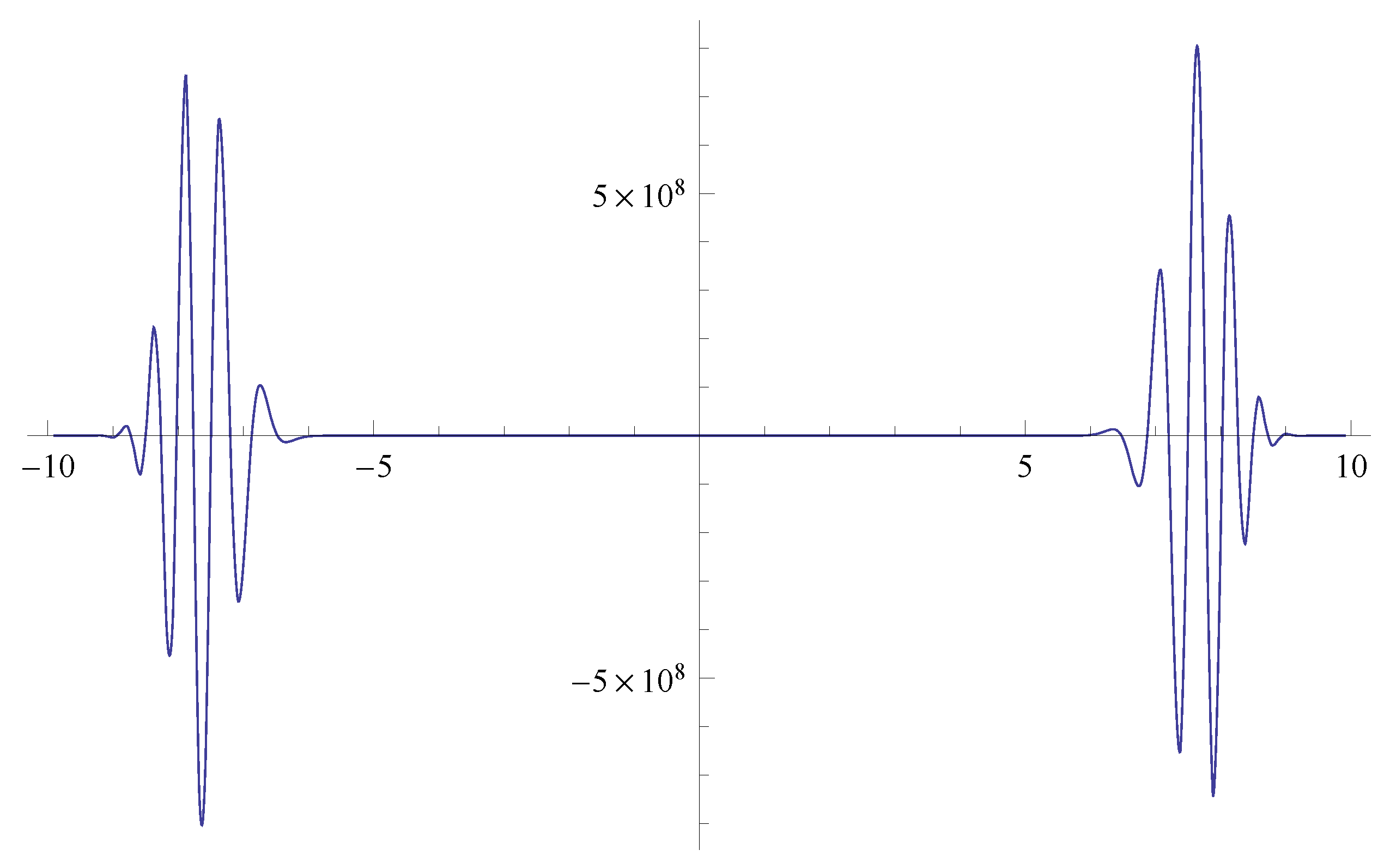
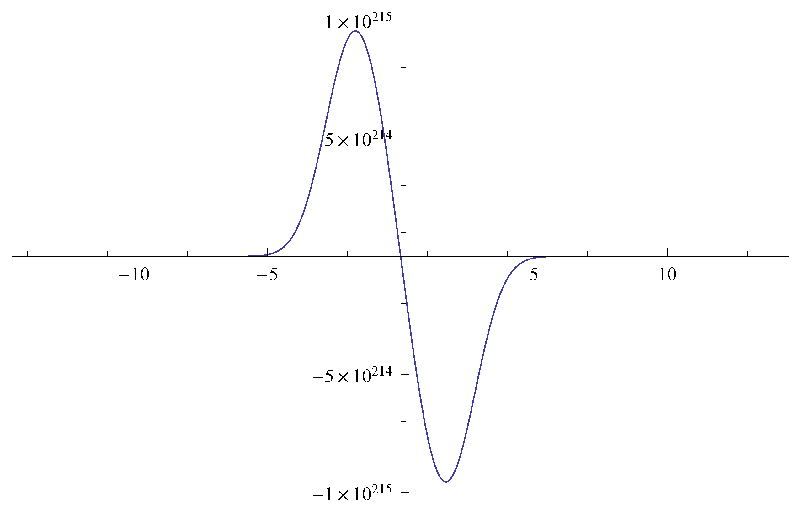
To computationally prove that the analytic solutions in terms of the Mittag–Leffler function are convergent, we give a brief review of its asymptotic behaviors; see [35] and the references therein. The short and long time behaviors of the Mittag–Leffler function are computed from the following special forms:

$$E_{\beta }(-t^{\beta })\sim \sum _{n=0}^{\infty }{(-1)}^n\frac{t^{n\beta }}{\mathrm{\Gamma }(n\beta +1)}\mathrm{as}t\ge 0.$$

(78)

This form is valid only for the short time. To deal with the long time, we have to compute the following function:

$$E_{\beta }(-t^{\beta })\sim \frac{sin\beta \pi }{\pi }\frac{\mathrm{\Gamma }\left(\beta \right)}{t^{\beta }}\mathrm{as}t\to \infty ,$$

(79)

and another useful form of the Mittag–Leffler function, namely:

$$E_{\beta }(-t^{\beta })\sim exp\left(\frac{-t^{\beta }}{\mathrm{\Gamma }[1+\beta ]}\right),$$

(80)

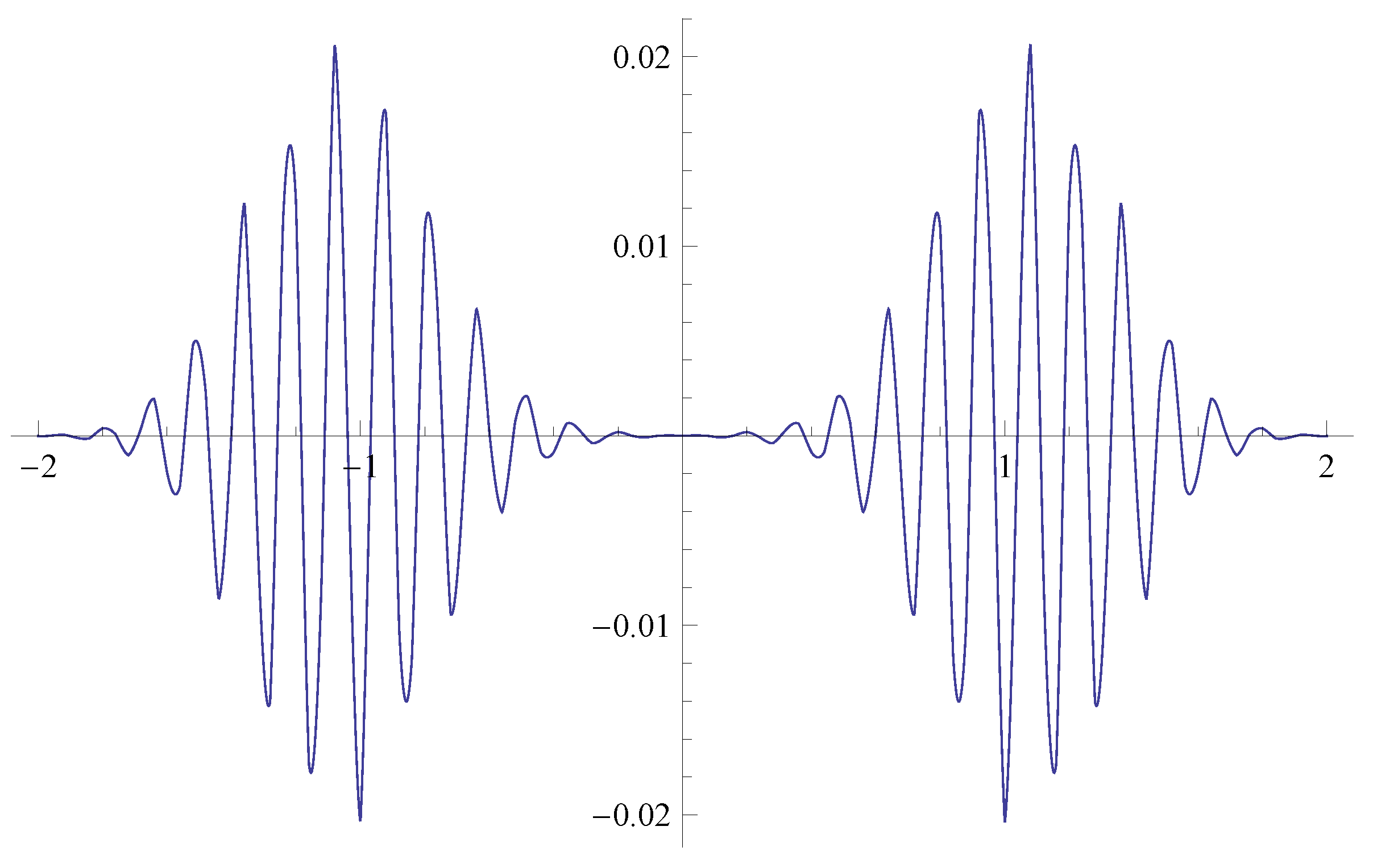
where this form is called the stretched exponential function. Substituting in this function with $\beta =1$, we obtain the fastest convergent function $e^{-t}$. Figure 1 and Figure 2 show the asymptotic behaviors of the Mittag–Leffler function for the short and long time. The $\mathrm{Hypergeometric}1\mathrm{F}1[1+n,2+n,-t]$ function is plotted in Figure 3 and is called the Kummer confluent hypergeometric function. 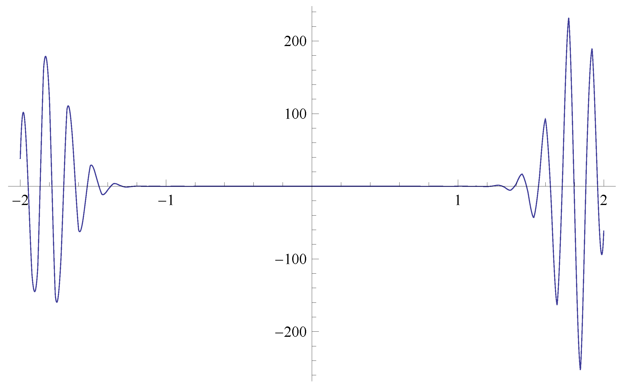It is known that $1F1$ is related to the convergent function $e^{-z}$ by the relation $1F1(1,1,-z)=e^{-z}$, for more details see [27,28]. Their time evolution is plotted in Figure 4. The simulation of these special functions indicates that the obtained analytic solutions are convergent as $t\to \infty$.

The time evolution of the approximate solution of the classical Equation (5), i.e., as $\gamma =2,\alpha =1,\beta =2$, $a\left(x\right)=1,b\left(x\right)=-x$ and $f\left(x\right)=sin\frac{\pi x}{L}$, is plotted in Figure 5, Figure 6, Figure 7 and Figure 8.

The time evolution of the approximate solution of Equation (5) is as $a\left(x\right)=a=1$, $b\left(x\right)=-bx=-x$, $k=1,\gamma =2,\beta =1.7,\alpha =0.7,r=100$, and $f\left(x\right)=sin\frac{\pi x}{2r+1}$ is plotted in Figure 9, Figure 10, Figure 11 and Figure 12. The figures shows that the approximate solution reaches its stationary solution very fast.

The time evolution of the approximate solution of Equation (5) for $a\left(x\right)=a=1$, $b\left(x\right)=-bx$, $\gamma =0.8$, $\beta =1.7$, $\alpha =1$, $k=0.7$ and $f\left(x\right)=\delta \left(x\right)$ is plotted in Figure 13, Figure 14, Figure 15 and Figure 16.

The time evolution of $y^{\left(n\right)}$ of the same equation, but corresponding to $\gamma =1$, $\beta =1.7$, $\alpha =1$, and $f\left(x\right)=sin\frac{\pi x}{L}$, is plotted Figure 17, Figure 18, Figure 19 and Figure 20. These simulations show that the approximate solution reaches its stationary solution at $t=20$, and it does not change even if we increase the number of iterations till we reach $t=60$. This is a necessary property of any stochastic process.

7. Conclusions

In this paper, we studied the classical wave equation with the damped term and associated with the stochastic Fokker–Planck operator. Two physical and biological models were studied as direct applications to this partial differential equation. The need to extend the time first-order derivative to the Caputo time-fractional operator was discussed. The need for the space-fractional operator was also discussed. The analytic solutions for the classical models were studied to illustrate that the special functions are very necessary, besides proving that the analytic solutions are not unique. The Laplace transform was implemented to obtain the solution of the time-fractional differential equation of three terms. The solution was given in terms of the Mittag–Leffler function and its nth derivative.

The explicit finite difference rules besides the Grünwald–Letnikov scheme were implemented to obtain the approximate solutions of the studied models. The simulation of the approximate solutions of the classical case and the space-time-fractional equations with different values of the fractional orders were presented. As stochastic processes, the approximate solutions do not change after reaching the stationary solution.