
The Influence Factor Analysis of Symmetrical Half-Bridge Power Converter through Regression, Rough Set and GM(1,N) Model

Department of Electrical Engineering, Chienkuo Technology University, Changhua 500, Taiwan
*
Author to whom correspondence should be addressed.
Axioms 2022, 11(1), 18; https://0-doi-org.brum.beds.ac.uk/10.3390/axioms11010018
Submission received: 21 October 2021
/
Revised: 30 December 2021
/
Accepted: 31 December 2021
/
Published: 2 January 2022
(This article belongs to the Special Issue Grey System Theory and Applications in Mathematics)
Abstract
:Analysis of power converter performance has tended to be engineering-oriented, focusing mainly on voltage stability, output power and efficiency improvement. However, there has been little discussion about the weight relations between these factors. In view of the previous inadequacy, this study employs regression, rough set and GM(1,N) to analyze the relations among the factors that affect the converter, with a symmetrical half-bridge power converter serving as an example. The four related affecting factors, including the current conversion ratio, voltage conversion ratio, power conversion ratio and output efficiency, are firstly analyzed and calculated. The respective relative relations between output efficiency and the other three factors are obtained. This research can be referred to by engineers in their design of symmetrical half-bridge power converters.
1. Introduction
Currently, two different models of power supply are available in the market, including linear power supply and switching power supply. Despite its simple circuit structure, high stability, small ripple, fast transient response, low electromagnetic interference and high reliability, linear power supply is associated with low efficiency and large size. A switching power supply is designed to compensate for the shortcomings of the linear power supply. Therefore, with technological advancements, the linear power supply has been gradually replaced by the switching power supply, which is widely used in 3C products. Despite switching power supply being credited with high conversion efficiency, light weight and a wide-range DC input, its circuit structure features a complex circuit and large electromagnetic interference. This study focuses on this phenomenon [1,2].
In this study, the symmetrical half-bridge power converter serves as a switching power supply. The symmetrical half-bridge power converter is different from push-pull single-ended driving or interleaved driving, which requires a double input voltage. It is widely used in converters whose power supply voltage is higher than the safety standard voltage value of the transistor.
Research on power converters has focused mainly on circuit design and practical development, including high-power two-way bridge power supplies [3]. A high-voltage switching resonant converter has been used to reduce switching loss in the system [4,5,6]. High-efficiency converters [7,8,9,10,11] and a reluctance motor drive system for the two-way voltage double front-end converter have been developed [12]. In battery charging applications [13,14,15,16], topology and design optimization were achieved in an optimized multiport DC/DC converter for transportation [17,18,19] and a PWM in a DC/DC converter [20,21]. Existing studies in the literature also include a passive RF-DC converter for energy harvesting at ultra-low input power at 868 MHz [22]; using extended Kalman filter observer technology to solve the fault problem in a DC/DC converter [23], as well as using a DC/DC converter for e-mobility charging [24]. Related to this study, the symmetrical half-bridge is related to high-power half-bridge converters [25,26,27]. However, little research deals with the integration of the three methods. This study, therefore, can be regarded as a pioneering study of converters [28].
The second section introduces the mathematics model employed, which includes regression analysis, the rough set method and the GM(1,N) model of grey system theory. Section 3 provides a field example of a symmetrical half-bridge power converter. Section 4 describes the complete calculation steps for the symmetrical half-bridge power converter. The final section draws conclusions from the results and puts forward suggestions for future research.
2. The Mathematical Model of Soft Computing
This section mainly describes the computing processes of regression analysis, rough set and grey GM(1,N) model. The procedure is described below.
2.1. Regression Analysis
Regression analysis is a method of statistically analyzing data. Its main purpose is to understand the relations between two or more variables and the direction and intensity of the correlation. It aims to establish a mathematical model to observe specific variables and predict the variables of interest. There are four steps in the calculation process [29,30].
1. List the equation
2. Expand Equation (1) to obtain
3. Transfer Equation (2) into matrix form
4. Use to find the value of , where
The value of is the weighting of .
2.2. Rough Set Method
Rough set is used for classification. For the affecting factors in the system, the weighting of each affecting factor to the output of the system can be obtained.
The analysis steps of rough set are as follows [31]:
1. Information system (IS)
- i.
- is called the universal set;
- ii.
- is called the attribute set.
2. Information function
- i.
- is called the domain of universal set;
- ii.
- is called the range.
3. Discrete: based on Equation (6).
- i.
- is the maximum value of the continuous attribute;
- ii.
- is the minimum value of the continuous attribute.
Through the discretization, one can obtain the attribute value
where is the representative value of discrete normalization, and k is called the grade of discreteness.
4. Lower approximation and upper approximation
The lower approximation means that the attribute factor is completely determined to belong to U (intersection), while the upper approximation means that the attribute factor may belong to U (union).
5. Indiscernibility: For any and , they are in the same category.
6. Positive, negative and boundary
7. Dependents: The dependence of decision attribute D on conditional attribute C is
Under the conditional attribute C, the ratio of objects that can be completely classified into the whole number of objects in the set is calculated.
8. Significant: Indicates the importance of attributes in the decision-making system.
2.3. GM(1,N) Model
As with rough set, the GM(1,N) model is used to find the weighting of each affecting factor to the output in the system. According to the definition of grey system theory, the grey differential equation of the model is [32]:
where:
- i.
- and are coefficients;
- ii.
- is a standard sequence;
- iii.
- are inspected sequences;
- iv.
- .
If in the sequence , is the main behavior of the system, and are the factors that affect the main behavior, the analysis step is as follows:
1. Build up original sequence
2. Build up AGO sequence
3. Transfer Equation (13) into a difference form
4. Based on Equation (14), we substitute the AGO data, and we obtain
Then, transfer Equation (15) into matrix form, as shown in Equation (16)
According to the least squares method, by using , we find the values
where:.
3. Real Example and Verification
This paper first designs seven sets of parameter values, and then provides a sample of symmetrical half-bridge power converters. The relevant measurement values are obtained through conducting experiments. The three input factors, which are the internal parameters of the converter, include the current conversion ratio, voltage conversion ratio and power conversion ratio. The output factor refers to the efficiency of the converter. Soft computing is employed to analyze the weighting relationship among the input factors and output factor [33].
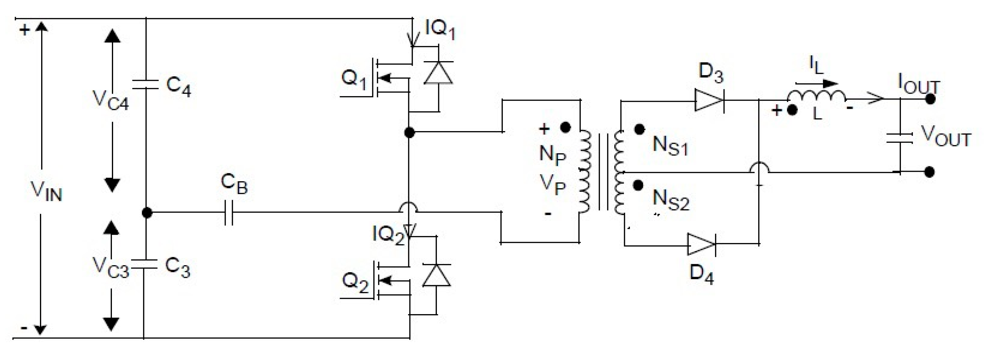
3.1. The Circuit of Symmetrical Half-Bridge Power Converter
The circuit of the symmetrical half-bridge power converter is shown in Figure 1.
3.2. The Experimental Data
The experimental values are shown in Table 1.
4. Calculation and Analysis
This section mainly explains the calculation process and results of three soft computing methods.
4.1. Regression Analysis
The analysis sequences are built based on the mathematics model.
Output efficiency: = (0.922, 0.944, 0.944, 0.944, 0.940, 0.935, 0.919)
The ratio of output current to input current (Io/Ii):
= (7.523810, 7.689024, 7.695122, 7.698171, 7.665049, 7.629779, 7.501695)
The ratio of output voltage to input voltage (Vo/Vi):
= (0.122684, 0.122619, 0.122619, 0.122645, 0.122594, 0.128994, 0.129019)
The ratio of output power to input power (Po/Pi):
= (0.944138, 0.944138, 0.944138, 0.939555, 0.934579, 0.918535, 0.921659)
Substitute into Equation (3) for weighting:
Use to find the values of , where:
The final results are shown in Table 3.
Regression analysis shows that the actual circuit is positively correlated, while the other two are negatively correlated.
4.2. Rough Set Method
Rough set must firstly discretize the values. Accordingly, this paper discretizes the measured values into four grades. Table 4 shows the result.
Table 4 indicates the ratio of output current to input current as R1, the ratio of output voltage to input voltage as R2, the ratio of output power to input power as R3 and efficiency as decision attribute D. Then, the discrete data are converted into the rough set model to calculate the significance of each attribute factor.
1. Calculate the attribute set ={{},{},{},{}}
2. Calculate the decision set ; hence, = {, and substitute into Equation (9) to obtain .
3. Analyze the conditional attributes of each factor
(1) Omit
Hence, = {}, and substitute into Equation (9) to obtain ; then, substitute into Equation (10) to obtain . Therefore, the significance of .
(2) Omit
Hence, = {{},{},{},{},{},{},{}}, and substitute into Equation (9) to obtain ; then, substitute into Equation (10) to obtain . Therefore, the significance of .
(3) Omit
Hence, = {{},{},{},{},{},{},{}}, and substitute into Equation (9) to obtain , and substitute into Equation (10) to obtain ; therefore, the significance of .
The final results are shown in Table 5.
4.3. GM(1,N) Method
1. The analysis sequences are built based on the mathematical model.
Output efficiency:
= (0.922, 0.944, 0.944, 0.944, 0.940, 0.935, 0.919)
The ratio of output current to input current (Io/Ii)
= (7.523810, 7.689024, 7.695122, 7.698171, 7.665049, 7.629779, 7.501695)
The ratio of output voltage to input voltage (Vo/Vi):
= (0.122684, 0.122619, 0.122619, 0.122645, 0.122594, 0.128994, 0.129019)
The ratio of output power to input power(Po/Pi)
= (0.944138, 0.944138, 0.944138, 0.939555, 0.934579, 0.918535, 0.921659)
2. Build up AGO sequence
= (0.922, 1.866, 2.81, 3.754, 4.694, 5.629, 6.548)
= (7.5238, 15.2128, 22.908, 30.6061, 38.2712, 45.901, 53.4026)
= (0.1227, 0.2453, 0.3679, 0.4906, 0.6132, 0.7422, 0.8712)
= (0.9441, 1.8883, 2.8324, 3.772, 4.7065, 5.6251, 6.5467)
= (1.394, 2.338, 3.282, 4.224, 5.1615, 6.0885)
3. Substitute into Equation (16) to obtain the weighting
Uses to find the values of weighting where: .
The final results are shown in Table 6.
5. Conclusions
Research on power converters in the past has turned out good results in circuit design and product development. The integration of regression analysis, rough set analysis and GM(1,N) can be regarded as a pioneering research method. The paper first develops a practical sample. By employing regression analysis, rough set and the GM(1,N) model, this study finds that the current conversion ratio has the greatest impact on efficiency. This finding is consistent with the basic principle of the power converter, which is the characteristic of current amplification. The analysis method implemented in this study, therefore, is reasonable.
This study analyzes only one of the symmetrical half-bridge power converters. Soft computing for classification, according to this research, is applicable to electrical engineering. A forthcoming study is suggested to aim at other types of power converters on the one hand, and to combine other related mathematical models to increase the integrity of the overall analysis on the other.
Author Contributions
Conceptualization, S.-K.C. and K.-L.W.; methodology, K.-L.W.; software, K.-L.W.; validation, S.-K.C.; formal analysis, K.-L.W.; investigation, S.-K.C.; resources, S.-K.C.; data curation, S.-K.C.; writing—original draft preparation, K.-L.W.; writing—review and editing, K.-L.W.; visualization, S.-K.C.; supervision, K.-L.W.; project administration, S.-K.C. and K.-L.W.; funding acquisition, S.-K.C. and K.-L.W. All authors have read and agreed to the published version of the manuscript.
Funding
This research was funded by Higher Education Sprout Project of Chienkuo Technology University grant number is 2021-06-02.
Institutional Review Board Statement
Not applicable.
Informed Consent Statement
Not applicable.
Conflicts of Interest
The authors declare no conflict of interest.
References
- Wu, Y.L. Switching Power Converter; Wensheng Book Store: New Taipei City, Taiwan, 2018. [Google Scholar]
- Head Line Daily, Topological Knowledge Collection of Half-Bridge and Full-Bridge Converters, Taipei. Available online: https://kknews.cc/zh-tw/society/revjzjo.html (accessed on 18 January 2017).
- Ma, G.; Qu, W.L.; Yu, G.; Liu, Y.Y.; Liang, N.G.; Li, W.Z. A zero-voltage- switching bidirectional DC-DC converter with state analysis and soft-switching- oriented design consideration. IEEE Trans. Ind. Electron. 2009, 56, 2174–2184. [Google Scholar]
- Chien, C.H. Zero-Voltage Switching Resonant Converters for High Input Voltage Applications. Ph.D. Thesis, Institute of Microelectronics, National Cheng Kung University, Tainan, Taiwan, 2013. [Google Scholar]
- Lin, B.R.; Lin, Y.K. An investigation into a ZVS resonant converter to achieve wide voltage operation. J. Innov. Technol. 2021, 3, 65–72. [Google Scholar]
- Qin, H. Wide-range high voltage input LLC auxiliary power supply. Int. Core J. Eng. 2021, 7, 291–298. [Google Scholar]
- Lin, B.R. Analysis of a DC converter with low primary current loss and balance voltage and current. Electronics 2019, 8, 439. [Google Scholar] [CrossRef] [Green Version]
- Ranganathan, S.A. Noyal Doss Mohan, Formulation and analysis of single switch high gain hybrid DC to DC converter for high power applications. Electronics 2021, 10, 2445. [Google Scholar] [CrossRef]
- Adly, M.; Strunz, K. Irradiance-adaptive PV module integrated converter for high efficiency and power quality in standalone and DC microgrid applications. IEEE Trans. Ind. Electron. 2018, 65, 436–446. [Google Scholar] [CrossRef]
- Ho, K.Y. Design and Implementation of an AC/DC Converter with High Efficiency and High Power Factor. Master’s Thesis, Department of Electrical Engineering, Chienkuo Technology University, Chunghua, Taiwan, 2015. [Google Scholar]
- Yeh, C.L. Conversion Efficiency Analysis for the Effect of Resonant Inductance in a Half-Bridge LLC Series Resonant Converter. Master’s Thesis, Department of Electrical Engineering, National Sun Yat-sen University, Kaohsiung, Taiwan, 2017. [Google Scholar]
- Chen, M.S. Design and Implementation of Bidirectional Voltage-Doubler Front-End Converter for Single-Sensor Switched Reluctance Motor Drives. Master’s Thesis, The College of Electrical Engineering and Computer Science, National Chiao Tung Universitym, Hsinchu, Taiwan, 2018. [Google Scholar]
- Lee, I.O.; Lee, J.Y. A high-power DC-DC converter topology for battery charging applications. Energies 2017, 10, 871. [Google Scholar] [CrossRef]
- Wu, X.W. Converter and control of bidirectional DC/DC converter for power battery testing. Int. Core J. Eng. 2020, 6, 375–385. [Google Scholar]
- Chakraborty, S.; Vu, H.N.; Hasan, M.M.; Tran, D.D.; el Baghdadi, M.; Hegazy, O. DC-DC converter topologies for electric vehicles, plug-in hybrid electric vehicles and fast charging stations: State of the art and future trends. Energies 2019, 12, 1569. [Google Scholar] [CrossRef] [Green Version]
- Szymanski, J.R.; Mortka, M.Z.; Wojciechowski, D.; Poliakov, N. Unidirectional DC/DC converter with voltage inverter for fast charging of electric vehicle batteries. Energies 2020, 13, 4791. [Google Scholar] [CrossRef]
- Tran, D.; Chakraborty, S.; Lan, Y.F.; Mierlo, J.V.; Hegazy, O. Optimized multiport DC/DC converter for vehicle drivetrains: Topology and design optimization. Appl. Sci. 2018, 8, 1351. [Google Scholar] [CrossRef] [Green Version]
- Lin, B.R.; Ko, M.C. Wide voltage range DC/DC converter for railway auxiliary power units. J. Innov. Technol. 2021, 3, 69–78. [Google Scholar]
- Wang, H.Y. Simulation research on energy storage bidirectional DC-DC converter in ship microgrids. Int. Core J. Eng. 2019, 5, 117–122. [Google Scholar]
- Sato, Y.S.; Uno, M.T.; Nagata, H.K. Nonisolated multiport converters based on integration of PWM converter and phase-shift-switched capacitor converter. IEEE Trans. Power Electron. 2020, 35, 2020. [Google Scholar] [CrossRef]
- Wang, C.M.; Lin, C.Y.; Wang, H.L. Analysis and design of a zero-voltage- switching PWM DC-DC converter without auxiliary circuit. J. Innov. Technol. 2021, 3, 1–5. [Google Scholar]
- Chaour, I.S.; Fakhfakh, A.; Kanoun, O. Enhanced passive RF-DC converter circuit efficiency for low RF energy harvesting. Sensors 2017, 17, 546. [Google Scholar] [CrossRef] [PubMed] [Green Version]
- Schmidt, S.; Oberrath, J.; Mercorelli, P.A. Sensor fault detection scheme as a functional safety feature for DC-DC Converters. Sensors 2021, 21, 6516. [Google Scholar] [CrossRef] [PubMed]
- Lee, J.H.; Park, S.J.; Lim, S.K. Improvement of multilevel DC/DC converter for e-mobility charging station. Electronics 2020, 9, 2037. [Google Scholar] [CrossRef]
- Wang, C.M. A novel single-stage high-power-factor electronic ballast with symmetrical half-bridge topology. IEEE Trans. Ind. Electron. 2008, 55, 969–972. [Google Scholar] [CrossRef]
- Tang, Y.; Blaabjerg, F.; Loh, C.L.; Jin, C. Decoupling of fluctuating power in single-phase systems through a symmetrical half-bridge circuit. IEEE Trans. Power Electron. 2015, 30, 1855–1865. [Google Scholar] [CrossRef]
- Changchien, S.K. Houng-Ming Lee and Hsiau-Hsian Nien, Applying rough set in the influence factor analysis of symmetrical half-bridge power converter. In Proceedings of the ICSSMET 2020, Chiayi, Taiwan, 26 November 2020; pp. 41–45. [Google Scholar]
- Wen, K.L.; You, M.L. Apply Soft Computing in Data Mining, 2nd ed.; Taiwan Kansei Information Association: Taichung, Taiwan, 2018. [Google Scholar]
- Chang, K.H.; Wang, J.R.; Wen, K.L. The analysis of influence factor in quad-rotor unmanned aerial vehicle by using regression method. J. Quant. Manag. 2017, 13, 5-1–5-9. [Google Scholar]
- Jian, J.L.; Huang, C.C.; Chen, H.C.; Wen, K.L. Apply regression analysis in correlation of influence factors on the power efficiency at electronic air circulation heaters. In Proceedings of the ICSSMET, Chiayi, Taiwan, 26 November 2020; pp. 31–35. [Google Scholar]
- Wen, K.L.; You, M.L. Rough Set-the Decision of Uncertainty. Wunan Publisher: Taipei, Taiwan, 2020. [Google Scholar]
- Wen, K.L.; You, M.L. The Grey Prediction and Its Application in Soft Computing; Taiwan Kansei Information Society: Taichung, Taiwan, 2019. [Google Scholar]
- Wu, C.E. Applying GM(0,N) Model to the Design of Forward Converter. Master’s Thesis, Department of Electrical Engineering, Chienkuo Technology University, Chunghua, Taiwan, 2018. [Google Scholar]
Figure 1.
The diagram of symmetrical half-bridge power converter.

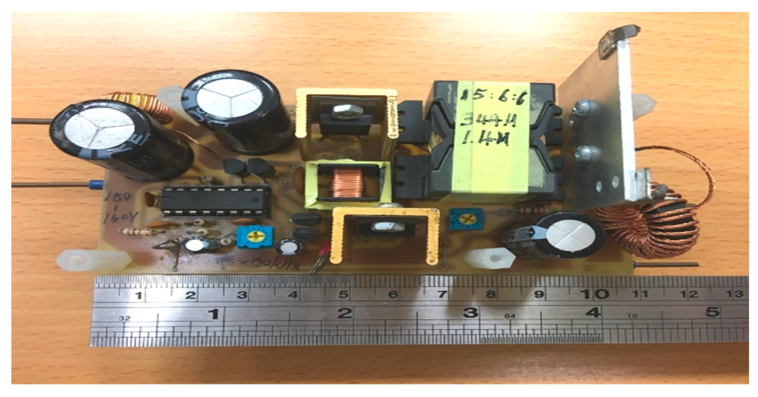
Figure 2.
The completed product of symmetrical half-bridge power converter.


Table 1.
The experimental values of symmetrical half-bridge power converter.
| Parameter | Ii (A) | Io (A) | Pi (W) | Vi (V) | Vo (V) | Po (W) | Duty Cycle (%) | Efficiency (%) |
|---|---|---|---|---|---|---|---|---|
| 01 | 0.084 | 0.632 | 13.02 | 155.0 | 19.016 | 12 | 35 | 92.2 |
| 02 | 0.164 | 1.261 | 25.42 | 155.0 | 19.006 | 24 | 35 | 94.4 |
| 03 | 0.246 | 1.893 | 38.13 | 155.0 | 19.006 | 36 | 35 | 94.4 |
| 04 | 0.328 | 2.525 | 50.84 | 155.0 | 19.010 | 48 | 35 | 94.4 |
| 05 | 0.412 | 3.158 | 63.86 | 155.0 | 19.002 | 60 | 35 | 94.0 |
| 06 | 0.497 | 3.792 | 77.04 | 155.0 | 19.994 | 72 | 35 | 93.5 |
| 07 | 0.590 | 4.426 | 91.45 | 155.0 | 19.998 | 84 | 35 | 91.9 |
Table 2.
The rearrangement of data of Table 1.
Table 2.
The rearrangement of data of Table 1.
| No. | Io/Ii | Vo/Vi | Po/Pi | |
|---|---|---|---|---|
| 01 | 7.523810 | 0.122684 | 0.944138 | 0.922 |
| 02 | 7.689024 | 0.122619 | 0.944138 | 0.944 |
| 03 | 7.695122 | 0.122619 | 0.944138 | 0.944 |
| 04 | 7.698171 | 0.122645 | 0.939555 | 0.944 |
| 05 | 7.665049 | 0.122594 | 0.934579 | 0.940 |
| 06 | 7.629779 | 0.128994 | 0.918535 | 0.935 |
| 07 | 7.501695 | 0.129019 | 0.921659 | 0.919 |
* Efficiency transfer to type of decimal point.
Table 3.
The final results of regression analysis.
| Parameter | |||
|---|---|---|---|
| Regression analysis | 0.1265 | −0.1437 | −0.0123 |
| Correlation | Positive correlation | Negative correlation | Negative correlation |
Table 4.
Discretization results of four grades.
| Group/Parameter | ||||
|---|---|---|---|---|
| 01 | 1 | 1 | 4 | 1 |
| 02 | 4 | 1 | 4 | 4 |
| 03 | 4 | 1 | 4 | 4 |
| 04 | 4 | 1 | 4 | 4 |
| 05 | 4 | 1 | 3 | 4 |
| 06 | 3 | 4 | 1 | 3 |
| 07 | 1 | 4 | 1 | 1 |
Table 5.
The final results of rough set under four grades.
| Grade/Parameter | |||
|---|---|---|---|
| Four grade | 0.8571 | 0 | 0 |
| Rank | 1 | 2 | 2 |
Table 6.
The final results of GM(1,N) model.
| Grade/Parameter | |||
|---|---|---|---|
| Weighting | 0.2478 | 0.2141 | 0.0091 |
| Rank | 1 | 2 | 3 |
Publisher’s Note: MDPI stays neutral with regard to jurisdictional claims in published maps and institutional affiliations. |
© 2022 by the authors. Licensee MDPI, Basel, Switzerland. This article is an open access article distributed under the terms and conditions of the Creative Commons Attribution (CC BY) license (https://creativecommons.org/licenses/by/4.0/).
Share and Cite
MDPI and ACS Style
Changchien, S.-K.; Wen, K.-L. The Influence Factor Analysis of Symmetrical Half-Bridge Power Converter through Regression, Rough Set and GM(1,N) Model. Axioms 2022, 11, 18. https://0-doi-org.brum.beds.ac.uk/10.3390/axioms11010018
AMA Style
Changchien S-K, Wen K-L. The Influence Factor Analysis of Symmetrical Half-Bridge Power Converter through Regression, Rough Set and GM(1,N) Model. Axioms. 2022; 11(1):18. https://0-doi-org.brum.beds.ac.uk/10.3390/axioms11010018
Chicago/Turabian StyleChangchien, Shih-Kuen, and Kun-Li Wen. 2022. "The Influence Factor Analysis of Symmetrical Half-Bridge Power Converter through Regression, Rough Set and GM(1,N) Model" Axioms 11, no. 1: 18. https://0-doi-org.brum.beds.ac.uk/10.3390/axioms11010018
Note that from the first issue of 2016, this journal uses article numbers instead of page numbers. See further details here.