
Local Optimality of Mixed Reliability for Several Classes of Networks with Fixed Sizes


1
School of Computer, Qinghai Normal University, Xining 810008, China
2
The State Key Laboratory of Tibetan Intelligent Information Processing and Application, Xining 810008, China
3
Academy of Plateau, Science and Sustainability, Xining 810008, China
4
Department of Mathematics, West Virginia University, Morgantown, WV 26506, USA
*
Author to whom correspondence should be addressed.
Axioms 2022, 11(3), 91; https://0-doi-org.brum.beds.ac.uk/10.3390/axioms11030091
Submission received: 17 January 2022
/
Revised: 20 February 2022
/
Accepted: 22 February 2022
/
Published: 24 February 2022
(This article belongs to the Special Issue Graph Theory with Applications)
Abstract
:In this work, the local optimality of mixed reliability of networks is surveyed. A reliability comparison criterion related with subgraphs to measure the local optimality of the mixed reliability of networks is established. Using the comparison criterion, we characterize all locally optimally mixed reliable networks among all n-vertex networks with fixed sizes , and , respectively.
1. Introduction
Throughout this paper, networks are modelled as graphs. All graphs considered here are simple and undirected. For positive integers m and n, an graph refers to a graph with n vertices and m edges. We shall use to denote the family of all graphs. For an integer , a graph G is k-connected if, for any pair of distinct vertices s and t of G, there are at least k internally disjoint s-t paths in G. The reliability of a network is defined as the probability that the residual vertices can communicate with each other. We shall use p and q to denote probabilities, and so unless otherwise stated, p and q will denote two real numbers (or real valued functions) with and . Generally, there are three kinds of reliability models: namely, the vertex fault model, the edge fault model, and the vertex-and-edge fault model, respectively. In the vertex fault model, it is assumed that all the edges will never fail, while the vertices could fail independently with the same failure probability p. Likewise, in the edge fault model, it is assumed that all vertices will never fail, while the edges could fail with the same failure probability q. Studies on the reliability in the vertex fault model and the edge fault model have been conducted by many researchers. In the Refs. [1,2,3], synthesis results of reliable networks in both the edge fault model and the vertex fault model were surveyed.
For the vertex fault model, Goldschmidt et al. in the Ref. [4] defined a network to be uniformly best if, for all choices of p, G is most reliable among all the graphs in , and showed that the complete bipartite graph is uniformly best among all graphs in . Furthermore, in the Ref. [4], the authors also showed that when , the star plus one edge and the cycle are the only two locally optimally reliable graphs of . Hakimi and Amin in the Ref. [5] studied the construction of reliable graphs with connectivity being , and with no more than n minimum vertex cut-sets. Smith et al. [6,7] showed how to construct locally optimally reliable graphs when the probability of a vertex failure is sufficiently small.
For the edge fault model, Bauer et al. [8,9] showed that for small edge failure probabilities and given the number of vertices and edges, all graphs having minimum chosen among those with maximum are locally optimally reliable, and studied the existence of such graphs. Zhao [10] showed that regular complete multipartite graphs and almost regular complete multipartite graphs are locally optimally reliable in their graph classes, respectively. Boesch et al. [11] showed that, given the number of vertices n, and the number of edges m, uniformly optimally reliable simple graphs always exist for , or , and proposed a conjecture for . Gross et al. [12] demonstrated that the uniformly optimally reliable simple graphs in these classes in the Ref. [11] were also uniformly optimally reliable when the classes were extended to include multigraphs. Wang [13] gave a proof of Boesch’s conjecture in the Ref. [11]. In the Ref. [14], the uniformly optimally and least reliable networks were given for the families of networks with n vertices, and edges. Liu et al. [15] proved that for any positive integer b, the complete tripartite graph is uniformly optimally reliable in its class . In 2014, Brown et al. [16] proved that uniformly optimally reliable graphs do not always exist. Petingi et al. [17] characterized uniformly least reliable graphs for m greater than or equal to . In the Ref. [18], the synthesis results of reliable networks were reviewed. Boesch et al. ([11]), Gross and Saccoman ([12]), and Chen and Zhao ([14]) also investigated the edge fault model, and independently verified the existence of uniformly optimally reliable graphs in the families of graphs , and . Nevertheless, Goldschmidt et al. in the Ref. [4] showed that with the vertex fault model, the above three families of graphs do not contain uniformly optimally reliable graphs.
Naturally, the vertex-and-edge fault model generalizes the two models above. In the vertex-and-edge fault model, it is assumed that the vertices would fail independently with probability p, and the edges would fail independently with probability q.
For the vertex-and-edge fault model, Evans and Smith [19] made a connection between the following two cases: small p, and small q, . Smith [20] showed that when p and q are small, a small-mixed-cut-set-optimal graph has the minimum unconnected probability among the graphs with given numbers of vertices and edges, and gave the method of how to construct these optimal graphs in many cases. Chen and He [21] in 2004 gave the upper and lower bounds of the mixed reliability of networks with unreliable vertices and edges. Mohamed [22] presented a new approach by using an efficient algorithm for evaluating the upper bound of the residual connectedness reliability of distributed systems with unreliable vertices and edges. For the case of the k-terminal connectivity criterion, Shpung, in the Ref. [23], used a Monte Carlo scheme to evaluate reliability for the networks with unreliable vertices and edges. Dash [24] used the artificial neural network in solving the network reliability optimization problem subjected to some total cost of the network, considering both edges and vertices of the network to be imperfect.
To the best of our knowledge, local optimality in mixed reliable networks has not been fully investigated. This motivates our current research. It has been known that the failure probabilities p and q are very small in real-life networks. Thus, the case when both p and q are close to 0 becomes very significant in practical applications. In this work, a reliability comparison criterion was established utilizing parameters related with subgraphs to measure the local optimality of the mixed reliability of networks. Using this comparison criterion, we characterize all locally optimally mixed reliable networks in with . Preliminaries will be shown in the next section. The comparison criterion is presented in Section 3. The characterizations of the locally optimally mixed reliable networks are obtained in the last two sections.
2. Preliminaries
Let be a graph with vertex set V and edge set E. In the edge fault model, the reliability of G [17] is defined by
where for all ℓ with , is the number of connected spanning subgraphs with ℓ edges of G.
Let i and j be integers with and . For a vertex subset and an edge subset with , let denote the subgraph obtained from G by deleting all vertices in and all edges in . If is disconnected, then is said to be an i-j mixed cut set of G. Let denote the number of i-j mixed cut sets in a graph G. It is shown in the Ref. [20] that, in the vertex-and-edge fault model, the disconnected probability of G, denoted by , can be expressed as
The mixed reliability of G is defined as . The two polynomials and are also called the mixed unreliability polynomial and the mixed reliability polynomial of G, respectively. Clearly, is a function on p and q.
Motivated by the definition of locally optimally reliable networks in the vertex fault model defined in the Ref. [4], we propose the following definition of locally optimally mixed reliable networks in the vertex-and-edge fault model.
Let denote two real numbers with and . When and , for a positive number , define .
Definition 1.
A graph G in is called locally optimally mixed reliable at , if there exists a real number such that the mixed reliability of G is greater than or equal to that of all other graphs in for all two-tuples .
3. Local Optimality of Mixed Reliability of Networks
For a graph and an integer , let denote the set of all connected subgraphs induced by i vertices of G, and be the number of connected induced subgraphs of G with i vertices. To emphasize the graph G, we often used and to denote the number of vertices and the number of edges of G, respectively. For an integer , the parameter of a graph G, which depends on the subgraphs of G, is defined as follows.
When , we have
and
Using the parameters above, a reliability comparison criterion is established to determine which graph is more locally mixed and reliable between any two graphs. Lemma 1 presents a formula to calculate the mixed reliability polynomial of networks.
Lemma 1.
Let G be a graph in and be the set of all connected induced subgraphs H of G ([10]). Then
Theorem 1.
Let n and m be two positive integers and let G and be two graphs in . Suppose that in the process of , there exist two positive real numbers and such that . If (a) , or (b) and , then .
Proof.
By assumption, in the process of , there exist two positive real numbers and such that , and it follows that
As , by Lemma 1, we have
where . Define
where is a polynomial on . Note that for any i, we have and . Therefore, using (3), we can write as follows.
Likewise, as , we have
Direct computation utilizing (4) and (5) yields the following:
It follows that if , then we have .
For the case of , since , we similarly have
It follows that if and , then . □
As a consequence of the definition of , we observe that
Theorem 2.
For any , . Furthermore, if and only if G is 2-connected.
4. Locally Optimally Mixed Reliable Networks in and
As any connected graph must be a graph with a unique cycle, a locally optimally mixed reliable graph is the cycle with n vertices. Thus, we consider graphs in .
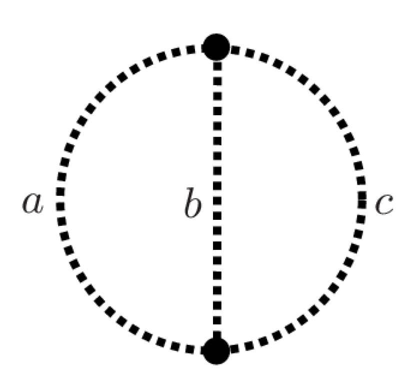
A chain in a graph is a path, each of whose internal vertex has a degree of exactly two in G and each of whose end vertices is of a degree larger than two. If two or more chains share the same two ends, then we say that these chains are parallel chains. The number of edges on a chain is called the length of the chain. For given positive integers and c, let denote the graph consisting of three parallel chains with lengths being , and c, respectively, as depicted in Figure 1.
Define . It is routine to verify that is the only class of 2-connected graphs in .
As shown in the next theorem, the following subfamily of is of particular interest:
Theorem 3.
A graph is a locally optimally mixed reliable network at if and only if .
Proof.
We first prove the necessity, and assume that is locally optimally mixed reliable at . By Theorems 1 and 2, we conclude that G lies in . Thus, there exist some integers with such that . Let . Then, is equal to the number of ways of removing one edge from any two of the three chains, respectively. Thus, . If the graph obtained by removing two vertices of is connected, then there are two different cases below.
Case 1. Remove two adjacent vertices in one chain. The numbers of ways for such a removal are m and in the cases of and , respectively.
Case 2. Remove one vertex of degree 2 from two chains, respectively. The number of ways for such removal is .
Summing up the two cases above, we have
Note that is equal to the number of ways to remove one vertex of degree 2 from one chain and one edge from another one. Hence, direct computation yields
It follows that can be expressed as follows.
By (7), we have
As , we conclude that . Therefore, if is with the maximum value among all , then we must have , and so . This completes the proof for the necessity.
To show the sufficiency, we assume that . Hence, by (6), there exists integers and c with and , and with . It follows by (1) that , and so by Theorem 2, . Since , it follows from (7) that . It then follows by Theorem 1 that G is a locally optimally mixed reliable network at . □
5. Locally Optimally Mixed Reliable Networks in
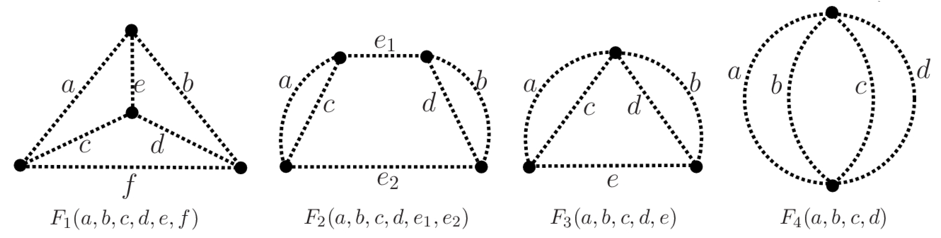
Chen and Zhao [14] showed that there are only four classes of 2-connected graphs in , denoted by , , and , respectively. To present the definitions of these graph families, we firstly introduce some notations. Let be positive integers. We define the graphs , , , as illustrated in Figure 2, respectively, where a dotted line in the graph represents a chain of the given length. Then we can define the related graph families as shown below.
The purpose of this section is to characterize networks in that are locally optimally mixed reliable at . We firstly investigate the necessity. By Theorems 1 and 2, if is locally optimally mixed reliable at , then G belongs to one of these graph families: Lemma 2 below investigates the locally optimally mixed reliable networks in . For notational convenience, we denote .
Lemma 2.
If is a locally optimally mixed reliable network at , then for any two numbers , we have .
Proof.
Suppose . The formula for is obtained from the following three cases.
Case 1. Remove two edges of . Since is equal to the number of ways of removing one edge from any two chains, respectively, we have
Case 2. Remove two vertices of . If the graph obtained by removing two vertices of is connected, then there are three subcases below.
Subcase 2.1. Remove two adjacent vertices in one chain. The number of ways for such removal is m.
Subcase 2.2. Remove one vertex of degree 2 from two chains, respectively. The number of ways for such removal is .
Subcase 2.3. Remove a vertex of degree 3 and a vertex of degree 2 such that the graph obtained is also connected. The number of ways for such removal is .
By computation, we obtain
Case 3. Remove a vertex and an edge of . If the graph obtained from by removing a vertex and an edge (which is not incident with the vertex removed) is connected, then there are two subcases below.
Subcase 3.1. Remove a vertex of degree 2 from one chain and an edge from another one. The number of ways for such removal is .
Subcase 3.2. Remove a vertex of degree 3 and an edge from the chain not containing the removed vertex. Then the number of ways for such removal is . Thus, we have
This leads to the following.
By (8), the following inequalities hold. If the largest difference for the lengths of any two chains with a common vertex is at least 2, say , then
If the largest difference for the lengths of any two chains without a common vertex is at least 2, say , then
Hence, if reaches the maximum value among all , then for any two numbers , we have . □
Suppose and , , . Let . In order to obtain the formula for , the following three cases need to be discussed.
Case 1. Remove two edges of . Note that is equal to the number of ways to remove two edges of such that the graph obtained from by removing these edges is connected. Then we have
Case 2. Remove two vertices of . If the graph obtained from by removing two vertices is connected, then there are three subcases below.
Subcase 2.1. Remove two adjacent vertices in one chain. Thus, the numbers of ways for such removal may be m, , and , respectively.
Subcase 2.2. Remove a vertex of degree 2 from two different chains, respectively. The number of ways for such removal is .
Subcase 2.3. Remove a vertex of degree 3 and a vertex of degree 2, respectively. The number of ways for such removal is . By computation, we get
where
Case 3. Remove a vertex and an edge of . If the graph obtained from by removing a vertex and an edge (which is not incident with the vertex removed) is connected, then there are two subcases below.
Subcase 3.1. Remove a vertex of degree 2 in one chain of and remove an edge in another chain. The number of ways for such removal is .
Subcase 3.2. Remove a vertex of degree 3 of and remove an edge in one chain. The number of ways for such removal is .
Thus, we have
By computation, the formula for is given by
where
Assume that with , . Let . By (9), in the case of and , we obtain
where
Assume that with . Let . By the same reason, we have
By comparing , , and , by (8)–(11), we have the following.
Lemma 3.
For and , then
Lemma 4.
For and , then
Lemma 5.
For , then
Motivated by the discussions above, we define a subfamily of as follows.
By Lemmas 3–5, we conclude that if is with the maximum value among all , then G is a member in . By Lemma 2, it holds that:
Lemma 6.
If is the locally optimally mixed reliable network at , then .
Theorem 4.
A graph is a locally optimally mixed reliable network at if and only if .
Proof.
As Lemma 6 justifies the necessity of the theorem, it suffices to prove the sufficiency. Suppose that . Then for some positive integers , satisfying such that any two of differ by one at most. With , it follows by (1) that , and so by Theorem 2, . Since any two of differ by at most one, by (8), we conclude that as well. Now by Theorem 1, G is a locally optimally mixed reliable network at , and so the sufficiency is also proved. □
6. Conclusions
The reliability of networks has become increasingly important, as the number of network applications in critical infrastructure and other social and management areas has been growing. In this paper, the vertex-and-edge fault reliability model was investigated and locally optimally mixed reliable networks in the vertex-and-edge fault reliability model were introduced and studied. A reliability comparison criterion was established to determine which one of two given networks with the same vertices and edges was more locally mixed and reliable. Furthermore, locally optimally mixed reliable networks in the graph families and were determined. For application purposes, it is expected to further understand locally optimally mixed reliable networks in other graph families. In this research, the parameters ’s were introduced, which have been successfully applied in studies of locally optimally mixed reliable networks in the graph families and . Future research can address the investigations of the roles these parameters, ’s, will play in studying network reliability, and the determination of locally optimally mixed reliable networks in the graph family when k becomes larger.
Author Contributions
Conceptualization, methodology, software, validation, writing—original draft preparation, writing—review and editing, L.D.; methodology, project administration, H.Z.; supervision, H.-J.L. All authors have read and agreed to the published version of the manuscript.
Funding
This research was funded by the State Key Laboratory of Tibetan Intelligent Information Processing and Application (Co-established by province and ministry), the Key Laboratory of Tibetan Information Processing Ministry of Education, Tibetan Information Processing Engineering Technology and Research Center of Qinghai Province, the Research Fund for the Chunhui Program of Ministry of Education of China, Qinghai-Tibet Plateau Innovation and Talent Introduction Base in Big Data Subject of Language and Culture (Grant No. 111Project D20035).
Institutional Review Board Statement
Not applicable.
Informed Consent Statement
Not applicable.
Data Availability Statement
Not applicable.
Conflicts of Interest
The authors declare no conflict of interest.
References
- Li, X. Current status and trends in the synthesis of reliable networks. Chin. J. Comput. 1990, 9, 699–705. [Google Scholar]
- Boesch, F.T.; Satyanarayana, A.; Suffel, C.L. A survey of some network reliability analysis and synthesis results. Networks 2009, 54, 99–107. [Google Scholar] [CrossRef]
- Boesch, F.T. On unreliability polynomials and graph connectivity in reliable network synthesis. J. Graph Theory 1986, 10, 339–352. [Google Scholar] [CrossRef]
- Goldschmidt, O.; Jaillet, P.; LaSota, R. On reliability of graphs with node failures. Networks 1994, 24, 251–259. [Google Scholar] [CrossRef] [Green Version]
- Hakimi, S.L.; Amin, A.T. On the design of reliable networks. Networks 1973, 3, 241–260. [Google Scholar] [CrossRef]
- Smith, D. Graphs with the smallest number of minimum cut sets. Networks 1984, 14, 47–61. [Google Scholar] [CrossRef]
- Smith, D.H.; Doty, L.L. On the construction of optimally reliable graphs. Networks 1990, 20, 723–729. [Google Scholar] [CrossRef]
- Bauer, D.; Boesch, F.; Suffel, C.; Tindell, R. Combinatorial optimization problems in the analysis and design of probabilistic networks. Networks 1985, 15, 257–271. [Google Scholar] [CrossRef]
- Bauer, D.; Boesch, F.T.; Suffel, C.; Slyke, R.V. On the validity of a reduction of reliable network design to a graph extremal problem. IEEE Trans. Circuits Syst. 1987, 34, 1579–1581. [Google Scholar] [CrossRef]
- Zhao, H.X. Research on Subgraph Polynomials and Reliability of Networks. Ph.D. Thesis, School of Computer, Northwestern Polytechnical University, Xi’an, China, 2004. [Google Scholar]
- Boesch, F.T.; Li, X.; Suffel, C. On the existence of uniformly optimally reliable networks. Networks 1991, 21, 181–194. [Google Scholar] [CrossRef]
- Gross, D.; Saccoman, J.T. Uniformly optimally reliable graphs. Networks 1998, 31, 217–225. [Google Scholar] [CrossRef]
- Wang, G.F. A proof of Boesch’s conjecture. Networks 1994, 24, 277–284. [Google Scholar] [CrossRef]
- Chen, M.M.; Zhao, L.C. Uniformly optimal and worst reliable networks. J. Petrochem. Univ. 2000, 13, 73–82. [Google Scholar]
- Liu, S.; Cheng, K.-H.; Liu, X. Network reliability with node failures. Networks 2000, 35, 109–117. [Google Scholar] [CrossRef]
- Brown, J.I.; Cox, D. Nonexistence of optimal graphs for all terminal reliability. Networks 2014, 63, 146–153. [Google Scholar] [CrossRef]
- Petingi, L.; Saccoman, J.T.; Schoppmann, L. Uniformly least reliable graphs. Networks 1996, 27, 125–131. [Google Scholar] [CrossRef]
- Boesch, F.T. Synthesis of reliable networks—A survey. IEEE Trans. Reliab. 1986, 35, 240–246. [Google Scholar] [CrossRef]
- Evans, T.; Smith, D. Optimally reliable graphs for both edge and vertex failures. Networks 1986, 16, 199–204. [Google Scholar] [CrossRef]
- Smith, D.H. Optimally reliable graphs for both vertex and edge failures. Comb. Probab. Comput. 1993, 2, 93–100. [Google Scholar] [CrossRef]
- Chen, Y.; He, Z. Bounds on the reliability of distributed systems with unreliable nodes & links. IEEE Trans. Reliab. 2004, 53, 205–215. [Google Scholar]
- Mohamed, H.S.; Yang, X.; Liu, H.; Wu, Z. An efficient evaluation for the reliability upper bound of distributed systems with unreliable nodes and edges. Int. J. Eng. Technol. 2010, 2, 107–110. [Google Scholar]
- Shpungin, Y. Combinatorial approach to reliability evaluation of network with unreliable nodes and unreliable edges. Int. J. Comput. Sci. 2006, 1, 177–182. [Google Scholar]
- Dash, R.K.; Barpanda, N.K.; Tripathy, P.K.; Tripathy, C.R. Network reliability optimization problem of interconnection network under node-edge failure model. Appl. Soft Comput. 2012, 12, 2322–2328. [Google Scholar] [CrossRef]
Figure 1.
The graph , where . Each dotted line represents a chain with the indicated length.

Figure 2.
Four graphs , , and . Each dotted line represents a chain with the indicated length.

Publisher’s Note: MDPI stays neutral with regard to jurisdictional claims in published maps and institutional affiliations. |
© 2022 by the authors. Licensee MDPI, Basel, Switzerland. This article is an open access article distributed under the terms and conditions of the Creative Commons Attribution (CC BY) license (https://creativecommons.org/licenses/by/4.0/).
Share and Cite
MDPI and ACS Style
Dong, L.; Zhao, H.; Lai, H.-J. Local Optimality of Mixed Reliability for Several Classes of Networks with Fixed Sizes. Axioms 2022, 11, 91. https://0-doi-org.brum.beds.ac.uk/10.3390/axioms11030091
AMA Style
Dong L, Zhao H, Lai H-J. Local Optimality of Mixed Reliability for Several Classes of Networks with Fixed Sizes. Axioms. 2022; 11(3):91. https://0-doi-org.brum.beds.ac.uk/10.3390/axioms11030091
Chicago/Turabian StyleDong, Lixin, Haixing Zhao, and Hong-Jian Lai. 2022. "Local Optimality of Mixed Reliability for Several Classes of Networks with Fixed Sizes" Axioms 11, no. 3: 91. https://0-doi-org.brum.beds.ac.uk/10.3390/axioms11030091
Note that from the first issue of 2016, this journal uses article numbers instead of page numbers. See further details here.