Article

CoreBug: Improving Effort-Aware Bug Prediction in Software Systems Using Generalized k-Core Decomposition in Class Dependency Networks

School of Computer Science and Information Engineering, Zhejiang Gongshang University, Hangzhou 310018, China
*
Author to whom correspondence should be addressed.
Submission received: 3 March 2022 / Revised: 17 April 2022 / Accepted: 24 April 2022 / Published: 27 April 2022

Abstract

:
Complex network theory has been successfully introduced into the field of software engineering. Many works in the literature have built complex networks in software, usually called software networks, to represent software structure. Such software networks and their related graph algorithms have been proved effective in predicting software bugs. However, the software networks used were unweighted and undirected, neglecting the strength and direction of the couplings. Worse still, they ignored many important types of couplings between classes, such as local variable, instantiates, and access. All of these greatly affect the accuracy of the software network in representing the topological detail of software projects and ultimately affect the metrics derived from it. In this work, an improved effort-aware bug prediction approach named CoreBug is proposed. First, CoreBug uses a weighted directed class dependency network (WDCDN) to precisely describe classes and their couplings, including nine coupling types and their different coupling strengths and directions. Second, a generalized k-core decomposition is introduced to compute the coreness of each class in the WDCDN. Third, CoreBug combines the coreness of each class with its relative risk, as returned by the logistic regression, to quantify the risk of a given class being buggy. Empirical results on eighteen Java projects show that CoreBug is superior to the state-of-the-art approaches according to the average ranking of the Friedman test.

1. Introduction

Software quality assurance (SQA) is of vital importance to the success of software projects, consuming a significant amount of resources (e.g., developers, time, and money). Unfortunately, software companies often have only limited resources for SQA activities. To make these activities resource-effective, many bug prediction approaches have been proposed to help prioritize the limited resources by identifying bug-prone software entities (e.g., files, methods, and classes). That is, limited resources should be allocated to the most bug-prone software entities first.
Bug prediction is often regarded as a binary classification problem with the aim of classifying software entities as buggy or clean. Many existing bug prediction approaches leverage machine learning techniques (e.g., logistic regression) to build classification models using a set of software metric values and some labeled data sets [1]. The existing approaches can be roughly categorized into two groups according to whether they consider the effort needed to inspect the code, i.e., the traditional prediction approaches (TPA) [1] and the effort-aware prediction approaches (EPA) [2]. In recent years, EPA has attracted a lot of attention, and many effective prediction models have been proposed [2,3].
Bug prediction approaches often rely on a set of software metrics to build prediction models. Thus, how to select a suitable set of metrics is a problem facing many researchers. Among the existing metrics, network metrics derived from the topological structure of software systems have attracted a lot of attention. Many researchers depict the software topology as a network, called software network [4,5], where nodes are software entities (e.g., files, methods, and classes), and edges (or links) are the couplings (e.g., inheritance, method call, and implements) between entities. Then, they borrow some metrics (e.g., degree, coreness, betweenness, and PageRank) from the field of network science to characterize the topological structure of software networks. These metrics have been gradually utilized to build prediction models [6,7,8,9].
Quite recently, Qu et al. [3] proposed an improved effort-aware bug prediction model, called top-core, that combines the coreness and relative risk of a class to quantify its risk of being buggy. The coreness values of the classes are derived from the software network using k-core decomposition. However, there still exist some unresolved problems in their work: (1) the software network they used was unweighted and undirected, neglecting the strength and direction of the couplings; and (2) they ignored many important types of couplings between classes, such as local variable, instantiates, and access. These two problems greatly affect the accuracy of the software network in representing the topological detail of software projects and ultimately affect the metrics (i.e., coreness) derived from it.
To tackle the above two problems in [3], we improved the work of Qu et al. in [10] by considering more coupling types to build a more accurate software network. However, we still did not consider the weights or direction of the edges, and the k-core decomposition used to compute the coreness only applies to unweighted undirected networks. In fact, the weights and direction correspond to the coupling strength and relationships between the components in the software. These interactions are indispensable. In order to make up for the shortcomings in the above two studies [3,10], an improved effort-aware bug prediction approach, called CoreBug, is proposed in this work. First, CoreBug uses a weighted directed class dependency network (WDCDN for short) to describe classes and their couplings, including nine coupling types and their different coupling strengths and directions. Second, a generalized k-core decomposition is introduced to compute the coreness of each class in the WDCDN, which takes into account the weight and direction of links. Third, CoreBug employs logistic regression to predict the relative risk of a class being buggy, which is further combined with the coreness of the class to quantify the final risk of the class being buggy. Empirical results on a set of eighteen Java projects show that CoreBug is superior to the state-of-the-art approaches according to the average ranking of the Friedman test.
In summary, we make the following contributions:
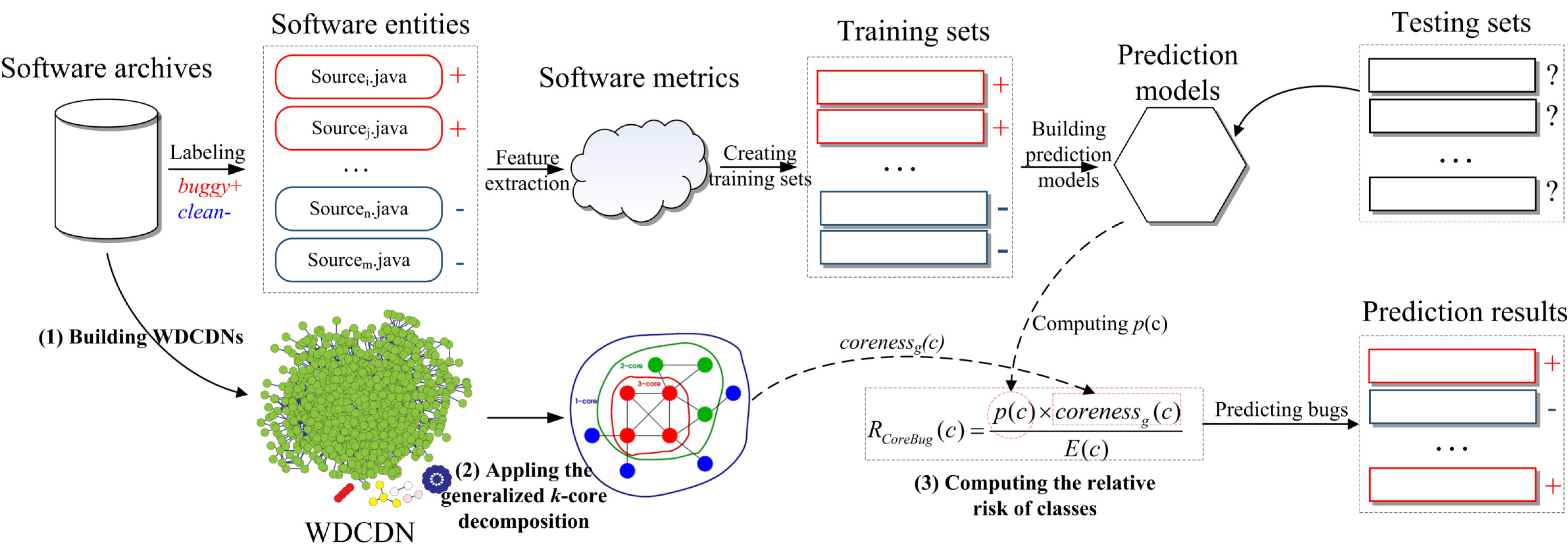
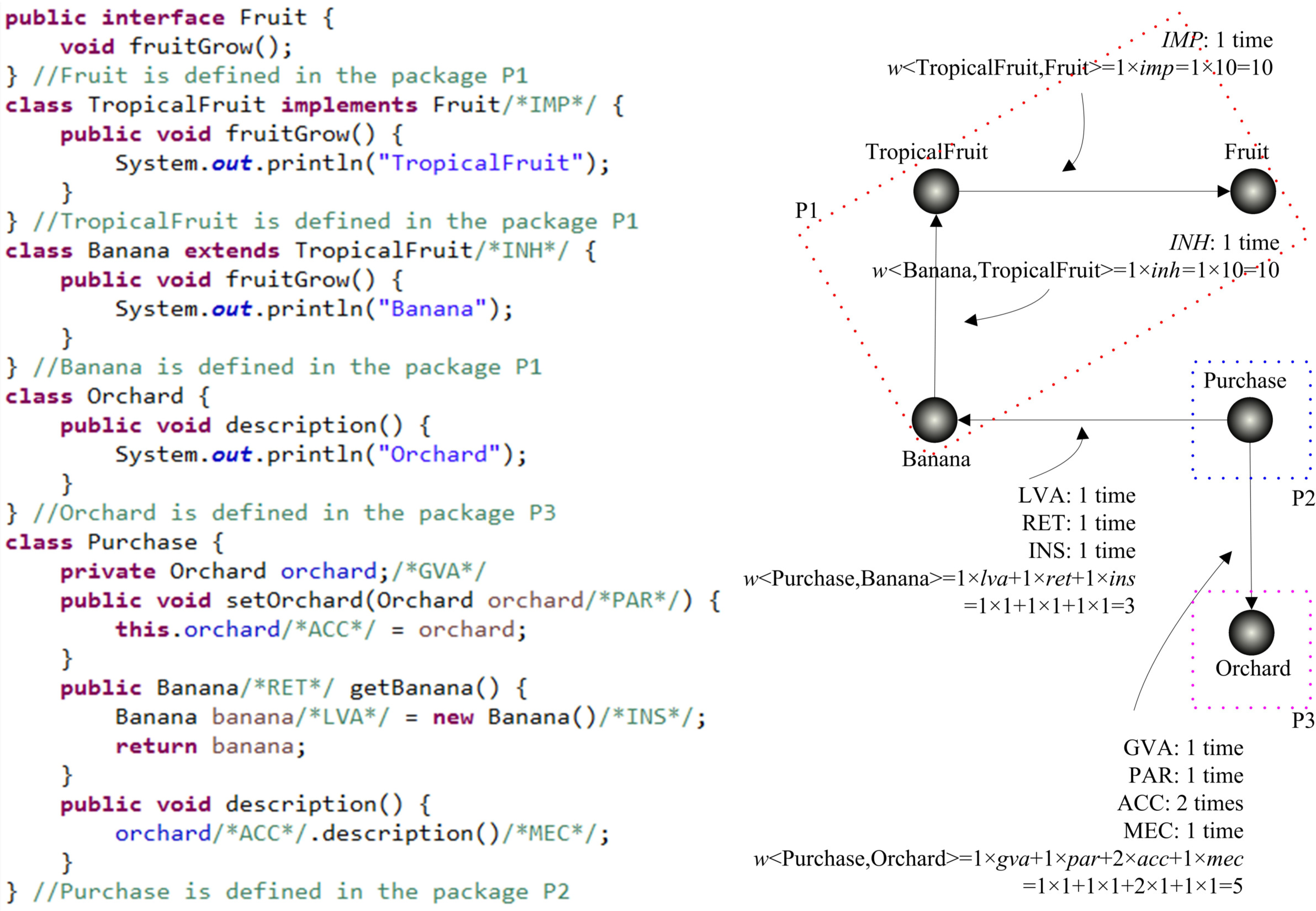
  • The work of Qu et al. [3] used unweighted undirected software networks to represent software structure at the class level. Worse still, their software networks only considered five coupling types between classes, neglecting many important couplings such as “instantiates”, “access”, and “method call”. It is a primitive representation that cannot precisely capture the couplings between classes. In this work, we propose a WDCDN that captures nine coupling types between classes, uses link weight to denote coupling strength and uses link direction to denote the coupling direction. In this sense, our WDCDN is a more accurate representation of the software structure when compared with the software network used in [3].
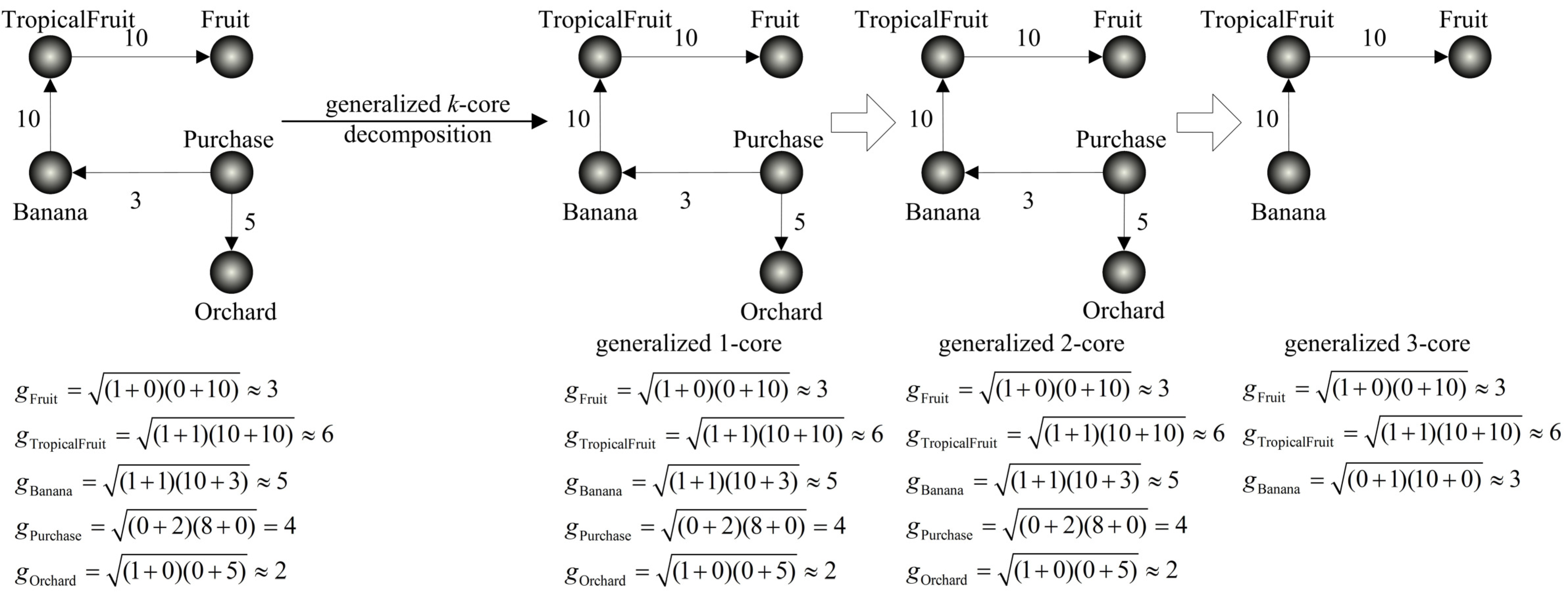
  • The work of Qu et al. [3] used k-core decomposition to compute the coreness of classes in the software network. This k-core decomposition can only be used in unweighted undirected networks. In this work, we apply a generalized k-core decomposition that can be used in weighted directed networks.
  • We perform a comprehensive set of experiments to validate the effectiveness of CoreBug.
The rest of this paper is organized as follows. Section 2 briefly reviews related work. Section 3 describes our CoreBug approach in detail, with a focus on the WDCDN that we used to represent the software structure, the generalized k-core decomposition that we used to compute the coreness of classes, the relative risk that we used to quantify the risk of a class being buggy, and the algorithm depicting the main steps of CoreBug. Section 4 empirically validates our CoreBug approach by comparing it with other state-of-the-art approaches. Section 5 concludes the paper and summarizes the proposed directions of our future work.

2. Related Work

In the last decade, to help managers effectively allocate limited resources (e.g., time and cost), many effective bug prediction models have been proposed. In this section, we focus on the research work performed from the perspective of complex networks and using complex network theory.
Zimmermann and Nagappan [11] used a set of network metrics computed on a function-level dependency graph to predict post-release bugs. They found that network metrics were correlated with the number of bugs in Windows Server 2003 and that these network metrics could be used to improve prediction performance. Pinzger et al. [7] proposed a developer-module network to represent developer contributions and applied several network centrality metrics (e.g., degree, closeness, and betweenness) to measure the fragmentation of developer contributions. They found that network centrality metrics were useful indicators for predicting fault-prone binaries and thus could be used to improve bug-prediction models. Meneely et al. [6] built a developer network derived from code churn information and used it to predict bugs at the file level. In their developer network, two developers were connected if they co-edited at least one file in a release. Then, some network metrics computed on the network were used as features for building prediction models. They reported that their model could reveal a large percentage of failures by examining a small percentage of files. Tosun et al. [12] replicated the work of [11] on five additional systems, and they revealed that, for large and complex systems, network metrics are useful indicators for predicting bugs, while for small-scale systems the effects of network metrics are not significant. Premraj and Herzig [13] replicated the work of [11] on three Java systems. They confirmed the effectiveness of network metrics in the scenario of post-release bug prediction, but they claimed that network metrics offered no advantage over code metrics in the scenarios of forward-release or cross-project bug prediction. Ma et al. [9] comprehensively evaluated the effectiveness of network metrics in the scenario of effort-aware bug prediction. They found that, although many network metrics are of practical value, their effects vary with different prediction settings and different systems. Chen et al. [8] evaluated network metrics in high severity fault-proneness predictions. They discovered that network metrics are correlated with high severity faults and have comparable predictive ability to code metrics. Qu et al. [14] applied node2vec to automatically learn a low-dimensional representation of a class dependency network. They revealed that this representation could be used to improve the performance of bug prediction models. Qu et al. [3] proposed a top-core approach to predict bugs in an effort-aware scenario. Their approach combined the coreness and relative risk of a class to quantify the risk of a class being buggy. The coreness of the classes was derived from the software network using k-core decomposition. They stated that their approach performed better than other approaches, such as R ee . However, Qu et al. did not sufficiently consider the coupling relationship or strength, and they constructed unweighted undirected networks. Such a representation does not match the characteristics of actual software. Pan et al. improved the work of [3] by considering more coupling relations. Guo et al. [15] proposed a random over-sampling mechanism to deal with the class imbalance problem in software defect prediction. Eken et al. [16] investigated the contribution of community smells on the prediction of bug-prone classes.
In summary, the existing work confirmed that network metrics are good indicators for predicting bugs and thus can be used to build prediction models. However, the existing works usually built unweighted or undirected networks, which cannot accurately capture the internal complexity of a software system. Our CoreBug approach is very similar to the top-core approach [3]. The only differences are (i) we used an accurate network representation that takes into account the link weight and link direction, and (ii) we applied generalized k-core decomposition to compute the coreness of classes.

3. The CoreBug Approach

Figure 1 gives the framework of our CoreBug approach, and the main steps are marked as (1)∼(3), that is, (1) building WDCDNs, (2) applying the generalized k-core decomposition, and (3) computing the relative risk of classes. In the following subsections, we describe these steps in detail.

3.1. Weighted Directed Class Dependency Network

The first task of CoreBug is to represent the software structure as a WDCDN since CoreBug needs the WDCDN to compute the coreness of each class. As mentioned in Section 1, WDCDNs actually encode the classes and their couplings in a system. Thus, to build the WDCDNs, CoreBug should extract the information regarding classes and their couplings from the source code of a subject system. In this work, this task is implemented by our own-developed software SNAP (Software Network Analysis Platform). Note that we only focus on software systems written in Java simply because the work of Qu et al. [3] only analyzed Java projects; consequently, our SNAP can currently only process Java projects.
Definition 1
(WDCDN). The WDCDN of a subject system is defined as WDCDN=(V,L,W), where V is the node set with v V denoting a specific class or interface, L = { u , v | u , v V u v w u , v 1 } is the link set with u , v L denoting a link from nodes u to v, and W = { w u , v | u , v L } is the weight set with w u , v denoting the weight on the link u , v .
A WDCDN uses links to denote the couplings between classes. In this work, nine types of couplings between classes are captured, i.e., inheritance (INH) relation (one class inherits from another class via the keyword extends), implements (IMP) relation (one class realizes one interface via the keyword implements), parameter (PAR) relation (methods in one class have at least one parameter with a type of another class), global variable (GVA) relation (one class has at least one field with a type of another class), local variable (LVA) relation (methods in one class have at least one local variable with a type of another class), return type (RET) relation (one class has at least one method with a return type of another class), instantiates (INS) relation (one class instantiates an object of another class), access (ACC) relation (one class has at least one method accessing a field with the type of another class), and method call (MEC) relation (one class has at least one method calling the method on one object of another class).
The weight on the link u , v , w u , v , is computed as
w u , v = T TS T u , v × t ,
where TS = { LVA , GVA , INH , IMP , PAR , RET , INS , ACC , MEC } is the set of coupling types, T u , v ( T TS ) denotes the frequency of coupling T between classes u and v, and t { lva , gva , inh , imp , par , ret , ins , acc , nec } denotes the strength of the corresponding coupling T.
Note that T u , v ( T TS ) can be resolved by tracing the occurrence of coupling type T in the source code. To estimate the coupling strength t for the corresponding coupling T, we apply the weighting mechanism proposed by Abreu et al. [17]. It is an objective weighting mechanism based on the distribution of inter- and intra-package couplings in the target Java project and can be computed by
t = 10 N intra T 0 N inter T = 0 1 N intra T = 0 N inter T = 0 r o u n d ( 0.5 + 10 × N intra T N intra T + N inter T ) o t h e r w i s e ,
where N intra T and N inter T denote the number of intra- and inter-package couplings of the coupling type T, respectively. r o u n d ( y ) returns an integer whose value is nearest to y.
For illustration purposes, we give a simple example (see Figure 2) to explain the coupling types that might exist between classes and show how to build a WDCDN from a Java snippet, including the nodes and links in a WDCDN and the weight on each link. In Figure 2, the left part is a simple Java code snippet, and the right part is its corresponding WDCDN.
In the WDCDN, we show the coupling types that each link denotes, the frequencies of each coupling type, and the final weight beside each link. Obviously, this code snippet contains four classes (i.e., TropicalFruit, Banana, Orchard, and Purchase), one interface (i.e., Fruit), and three packages (i.e., P1, P2, and P3). Fruit, TropicalFruit, and Banana are defined in P1; Purchase is defined in P2; and Orchard is defined in P3. Thus, the final WDCDN contains five nodes denoting the four classes and one interface. Furthermore, the four classes and one interface are coupled with each other via ten couplings, which have been explicitly annotated with comments /**/ in the code snippet. These comments locate the positions where the couplings occur. For example, the code line class TropicalFruit implements Fruit indicates that there is one instance of IMP coupling from class TropicalFruit to interface Fruit. Thus, there is a link between the nodes denoting TropicalFruit and Fruit. Other links in the WDCDN can be established in a similar way.
The weight on each link is computed by Equation (1). Take the weight on the link Purchase , Adaptor as an example. Since all three couplings, LVA, RET, and INS, occur only once, the weight on the link is w Purchase , Adaptor = 1 × lva + 1 × ret + 1 × ins . The values of lva , ret , and ins are computed using Equation (2). As mentioned above, the LVA coupling occurs only once between Purchase and Banana, and Purchase and Banana are defined in two separate packages P2 and P1, respectively. Thus, N intra LVA = 0 and N inter LVA = 1 . Hence, l v a = r o u n d ( 0.5 + 10 × 0 0 + 1 ) = 1 . In a similar way, we obtain r e t = r o u n d ( 0.5 + 10 × 0 0 + 1 ) = 1 and i n s = r o u n d ( 0.5 + 10 × 0 0 + 1 ) = 1 . Thus, w Purchase , Adaptor = 1 × lva + 1 × ret + 1 × ins = 1 × 1 + 1 × 1 + 1 × 1 = 3 . The weight on other links can be similarly computed.

3.2. Generalized k-Core Decomposition

CoreBug leverages generalized k-core decomposition ( G k c o r e for short) [18] to compute the coreness of each class in the WDCDN. We briefly introduce G k c o r e and some related concepts herein. Interested readers can refer to our previous work [18] for more details.
G k c o r e is proposed for computing the coreness of nodes in weighted directed networks. It is based on the generalized degree of node i, g i , which is defined as
g i = h i h i h i < 0.5 h i o t h e r w i s e ,
subject to
h i = ( k i i n + k i o u t ) ( j = 1 k i o u t w i , j + l = 1 k i i n w l , j ) ,
where h i is an intermediary to compute g i ; k i in and k i out are the traditional in- and out-degree of node i, respectively; and j = 1 k i out w i , j and l = 1 k i in w l , i are the weighted in- and out-degree of node i, respectively.
For a weighted directed graph (or network) G = ( V , E ) with | V | = n nodes and | E | = e links, some related concepts can be defined as follows.
Definition 2
(Generalized k-Core). A subgraph H = ( C , E | C ) induced by the set C V is a generalized k-core if and only if g v k ( v C ), and H is the maximum subgraph with this property.
G k c o r e applies a pruning routine to obtain the generalized k-core by recursively removing all nodes whose g v < k ( v C ), until all nodes in the remaining graph (or network) have generalized degree k .
Definition 3
(Generalized Coreness). If node i belongs to the generalized k-core but not to the generalized (k+1)-core, then the generalized coreness of node i, c o r e n e s s g ( i ) , is k.
We illustrate the process of G k c o r e using the WDCDN shown in Figure 2 when it is divided into a generalized k-core structure (see Figure 3). As shown in Figure 3, the left-most part is the WDCDN we built in Figure 2. First, we compute the g i ( i { Fruit , TropicalFruit , Banana , Purchase , Orchard } ) and remove from the network all nodes whose g i < 1 to obtain the generalized 1-core. In the WDCDN, because g i 1 ( i { Fruit , TropicalFruit , Banana , Purchase , Orchard } ), no nodes should be removed to obtain the generalized 1-core. Subsequently, we remove from the generalized 1-core all nodes whose g i < 2 to obtain the generalized 2-core. In the WDCDN, because g i 2 ( i { Fruit , TropicalFruit , Banana , Purchase , Orchard } ), no nodes should be removed to obtain the generalized 2-core. Again, we remove from the generalized 2-core all nodes whose g i < 3 to obtain the generalized 3-core. Because g O r c h a r d < 3 , node Orchard is removed from the generalized 2-core. We recompute the g i ( i { Fruit , TropicalFruit , Banana , Purchase } ) and repeat the remove-recompute procedure iteratively until only nodes whose g i 3 are left on the network. Thus, we obtain the generalized 3-core. This routine is applied until there are no nodes remaining in the network.
Based on the generalized k-core structure of the example WDCDN, we can obtain the generalized coreness of each node. Specifically, the generalized coreness of both Purchase and Orchard is 2, because they belong to the generalized 2-core but not to the generalized 3-core. Similarly, the generalized coreness of Fruit, TropicalFruit, and Banana is 3, because they belong to the generalized 3-core but not to the generalized 4-core.

3.3. The Relative Risk of Classes

The relative risk is usually used to quantify the risk of a class of being buggy. In CoreBug, the relative risk of class c, R CoreBug ( c ) , is defined as
R CoreBug ( c ) = p ( c ) × coreness g ( c ) E ( c ) ,
where p ( c ) is the probability of that class c being buggy, coreness g ( c ) is the generalized coreness of class c, and E ( c ) is the effort that should be expended to inspect class c. E ( c ) is estimated using line of code (LOC for short).
In this work, p ( c ) is predicted using the widely used machine learning technique, logistic regression. The reasons we choose logistic regression are twofold: (i) compared with other sophisticated approaches to building bug-prediction models, logistic regression is simple yet competitive [19]; (ii) logistic regression is not significantly different from other sophisticated approaches in terms of performance and thus is sufficient to build prediction models [20]. In this work, logistic regression is implemented using the scikit-learn framework (http://scikit-learn.org/stable/ (accessed on 3 January 2022)) and tuned using the grid search function.
Note that for a specific Java project, our training set is composed of a set of classes, each of which contains a set of software metrics (e.g., CK metrics, MOOD metrics, and LK metrics) and a label to signify whether it is buggy or clean. Then, the classes under analysis are ranked according to their R CoreBug ( c ) (c is a specific class) in descending order. Obviously, our model has the potential to rank the classes with high risk and less effort at the top of the ranked list of suspicious classes. We use an effort threshold, effort t { 20 % , 30 % , 40 % } , to identify the real bugs; effort t = LOC inspected LOC total , where LOC inspected is the inspected LOC, and LOC total is the total LOC.

4. Empirical Evaluation

In this section, to validate the effectiveness of our CoreBug approach, we design and conduct a series of experiments. The following subsections describe the research question we focus on, the subject systems we analyze, the baseline approaches, the metrics we use to compare different approaches, and the experiment results and analysis. All our experiments are performed on a Windows PC with Intel (R) Core (TM) i5-10400F CPU @ 2.90 GHz and 16 GB RAM.

4.1. Research Questions

In this work, we focus on the following research question (RQ):
RQ:
Does CoreBug perform better than the baseline approaches? CoreBug improved on top-core in two aspects, that is, a much more accurate representation of the software structure (i.e., WDCDN) and the generalized k-core decomposition to compute the coreness of classes in the WDCDN. Thus, we want to examine whether our CoreBug approach performs better than the baseline approaches in Section 4.3.

4.2. Subject Systems

Our subject systems consist of eighteen open-source Java projects that are widely used in the literature as benchmark systems (see Table 1). As mentioned above, our work relies on the source code of a subject system to compute the generalized coreness of each class. Thus, we collect the source code of these subject projects from their websites. To build the models to predict p ( c ) , our work relies on all classes in a target project, containing the name of the classes, a set of software metric values for the classes, and a label to signify whether the corresponding class is buggy. Such a data set is directly downloaded from publicly available software bug repositories. Specifically, the data sets for the first eight subject projects (i.e., Camel, Ivy, Log4j, Poi, Synapse, Tomcat, Velocity, and Xalan) are directly downloaded from the PROMISE repository [21], the data sets for the next three subject projects (i.e., Eclipse JDT Core, Equinox framework, and Lucene) are downloaded from the bug prediction dataset provided by D’Ambros et al. [22], and the data sets for the last seven subject projects (i.e., DrJava, GenoViz, HtmlUnit, Jmol, Jikes RVM, Jppf, and Jump) are downloaded from Shippey et al.’s data set [23].
Table 1 shows the versions of the subject projects that we analyzed, LOC (lines of code) of the software projects, #class (number of classes) in the corresponding WDCDNs, the percentage of buggy classes, and the websites to download the source code of these projects. Note that LOC is the practical lines of code, excluding comment lines and blank lines; #class contains the number of classes, inner classes, interfaces, and enum types.

4.3. Baseline Approaches

We choose two approaches in the field of effort-aware bug prediction, i.e., R ee  [2] and top-core [3], as baseline approaches. The two approaches can be differentiated by the relative risk metrics that they use to quantify the risk of a class of being buggy.
In R ee , the relative risk of class c, R R ee ( c ) , is defined as
R R ee ( c ) = p ( c ) E ( c ) ,
whereas in top-core, the relative risk of class c, R top core ( c ) , is defined as
R top core ( c ) = p ( c ) × coreness E ( c ) ,
where p ( c ) and E ( c ) have the same meanings as in Equation (5), and coreness is the coreness of class c computed by k-core decomposition.
Note that in the models of R ee and top-core, p ( c ) is also predicted using logistic regression. The reasons are discussed in Section 3.3.

4.4. Evaluation Metrics

To evaluate the performance of different approaches, P o p t is used as the evaluation metric. P o p t is widely-used in effort-aware bug prediction and is defined as
P opt ( m ) = 1 Area ( optimal ) Area ( m ) Area ( optimal ) Area ( worst ) ,
where Area ( optimal ) , Area ( m ) , and Area ( worst ) are the areas under the LOC-based cumulative lift charts corresponding to the optimal model, the prediction model m, and the worst model, respectively. In the optimal model, classes are ranked in descending order according to their bug density; in the worst model, classes are ranked in ascending order according to their bug density. m denotes a specific effort-aware prediction approach (e.g., BugCore and the baseline approaches).

4.5. Experiment Results and Analysis

We perform the experiments in the cross-validation scenario and use threefold (3 × 3) cross-validation. Note that P o p t is computed at a specific threshold effort t . For a specific software project, we repeat our experiments more than t times, and terminate the repetition when ( | P o p t t ¯ P o p t t 1 ¯ | < ε ) , where P o p t t ¯ = i = 1 t P o p t i t , P o p t i is the P o p t obtained in the i-th independent run, and ε is a small value, controlling the convergence level of the P o p t . In our experiments, ε = 0.0001 .
In this section, we show the results obtained on the subject systems (see Table 2, Table 3 and Table 4). In each of the following tables, we show the P opt t ¯ of different models (see columns R ee , top-core, and CoreBug) when applied to different software projects at a specific effort t . The largest P opt t ¯ value in each row is shown in bold. The last row in each table summarizes the Win/Tie/Loss results of CoreBug when compared with Ree and top-core. For example, in Table 2, CoreBug performs better than top-core on 11 subject projects (i.e., Win: 10), and there are only 7 subject projects where CoreBug performs worse than top-core (i.e., Loss: 7). There are no subject projects where CoreBug and R e e do not have significant differences (i.e., Tie: 0).
On the whole, there are a total of 54 (18 (the number of software projects)×3 (the number of thresholds)) experiments, and in 51.85% ( 10 + 9 + 9 54 ) of the experiments, CoreBug is better than R e e , while CoreBug is inferior to R e e only in about 48.15% ( 8 + 9 + 9 54 ) of the experiments. Furthermore, in about 57.41% ( 11 + 11 + 9 54 ) of the experiments, CoreBug is better than top-core, while in 42.59% ( 7 + 7 + 9 54 ) of the experiments, CoreBug is inferior to top-core.
Obviously, our CoreBug approach does not perform best in all subject systems, which compels us to examine the performance of different approaches (i.e., R ee , top-core, and CoreBug) in the whole data set. To this end, the Friedman test [24] is used to compare different approaches, and the results are shown in Table 5. We use P o p t t ¯ as a metric for comparing different approaches. It is a metric for which large values indicate a better approach. For such a metric, the Friedman test returns a small ranking value for a better approach. Thus, the three approaches can be sorted in the following order: CoreBug, top-core, and R ee , that is, CoreBug performs best, and R ee performs worst.
Answer to the RQ: Our results on a set of eighteen subject systems show that CoreBug is superior to the state-of-the-art approaches (i.e., R ee and top-core) according to the average ranking of the Friedman test.

4.6. Threats to Validity

There are several factors that may influence the validity of our conclusions. In this section, we discuss these threats.

4.6.1. Threats to Internal Validity

One internal threat lies in the accuracy of the network that we built for the target systems, which may affect the accuracy of the coreness for classes. We believe this threat has been minimized, as the SNAP tool we use has been sufficiently tested, and it has been used several times in our published papers [10]. To promote the replication of our work, we provide an online replication package that is publicly available via https://github.com/duxin1211/CoreBug_Axioms, accessed on 3 January 2022.

4.6.2. Threats to External Validity

In the experiments, there are several factors that may influence our conclusions. The first one is the threshold for the effort rate. In this work, we set the thresholds for effort to 20%, 30%, and 40%, which were determined by the distribution of defects [3,10]. However, when the threshold becomes larger, more classes are checked, which leads to an increase in the number of bugs detected by the approach. The consequence of this situation is that it is difficult to find a performance gap between our approach and other approaches. The second potentially limiting factor is that we used Java software systems as our subjects in this work. Thus, the conclusions obtained in this work suffer from the risks of being extended to systems developed in non-Java languages, such as C, C++, and Python. In future work, we will extend our approach to non-Java software systems.

5. Conclusions and Future Work

In this work, we propose an improved effort-aware bug prediction model that is based on a weighted directed software network (i.e., WDCDN) and generalized k-core decomposition. Our approach addresses the limitations of the state-of-the-art approach (i.e., top-core). Specifically, our approach takes into account more coupling types when constructing the network, which enables us to describe the software structure more accurately. Then, to better fit the two properties of weighted directed software networks, we introduce a generalized k-core decomposition method that takes into account not only the weights but also the directions of the links when calculating the coreness of class nodes in the network. The empirical results of experiments conducted using logistic regression on eighteen Java projects show that our approach is superior to the baseline approaches according to the average ranking of the Friedman test. In the future, we will validate our approach using a wide variety of non-Java or commercial software projects, and we will apply our method to more subject systems.

Author Contributions

Conceptualization, X.X., and W.P.; methodology, W.P., and X.X.; software, X.D., T.W., and X.X.; supervision, W.P., C.C., B.J., and J.W.; writing–original draft, X.D., T.W., and X.X.; writing–review and editing, X.D., T.W., X.X., L.W., and W.P. All authors have read and agreed to the published version of the manuscript.

Funding

This work was supported by the Natural Science Foundation of Zhejiang Province (Grant No. LY22F020007), and the Key R&D Program of Zhejiang Province (Grant Nos. 2019C01004 and 2019C03123).

Data Availability Statement

The data used to support the findings of this study are available from the corresponding author upon request.

Acknowledgments

The authors gratefully acknowledge all the reviewers for their positive and valuable comments and suggestions regarding our manuscript.

Conflicts of Interest

The authors declare that there are no conflicts of interest regarding the publication of this paper.

References

  1. He, P.; Li, B.; Liu, X.; Chen, J.; Ma, Y. An empirical study on software defect prediction with a simplified metric set. Inf. Softw. Technol. 2015, 59, 170–190. [Google Scholar] [CrossRef] [Green Version]
  2. Yang, Y.; Zhou, Y.; Lu, H.; Chen, L.; Chen, Z.; Xu, B.; Leung, H.K.N.; Zhang, Z. Are Slice-Based Cohesion Metrics Actually Useful in Effort-Aware Post-Release Fault-Proneness Prediction? An Empirical Study. IEEE Trans. Softw. Eng. 2015, 41, 331–357. [Google Scholar] [CrossRef]
  3. Qu, Y.; Zheng, Q.; Chi, J.; Jin, Y.; He, A.; Cui, D.; Zhang, H.; Liu, T. Using K-core Decomposition on Class Dependency Networks to Improve Bug Prediction Model’s Practical Performance. IEEE Trans. Softw. Eng. 2021, 47, 348–366. [Google Scholar] [CrossRef]
  4. Pan, W.; Li, B.; Liu, J.; Ma, Y.; Hu, B. Analyzing the structure of Java software systems by weighted K-core decomposition. Future Gener. Comput. Syst. 2018, 83, 431–444. [Google Scholar] [CrossRef]
  5. Li, H.; Wang, T.; Pan, W.; Wang, M.; Chai, C.; Chen, P.; Wang, J.; Wang, J. Mining Key Classes in Java Projects by Examining a Very Small Number of Classes: A Complex Network-Based Approach. IEEE Access 2021, 9, 28076–28088. [Google Scholar] [CrossRef]
  6. Meneely, A.; Williams, L.A.; Snipes, W.; Osborne, J.A. Predicting failures with developer networks and social network analysis. In Proceedings of the 16th ACM SIGSOFT International Symposium on Foundations of Software Engineering, Atlanta, GA, USA, 9–14 November 2008; Harrold, M.J., Murphy, G.C., Eds.; pp. 13–23. [Google Scholar] [CrossRef] [Green Version]
  7. Pinzger, M.; Nagappan, N.; Murphy, B. Can developer-module networks predict failures? In Proceedings of the 16th ACM SIGSOFT International Symposium on Foundations of Software Engineering, Atlanta, GA, USA, 9–14 November 2008; Harrold, M.J., Murphy, G.C., Eds.; pp. 2–12. [Google Scholar] [CrossRef] [Green Version]
  8. Chen, L.; Ma, W.; Zhou, Y.; Xu, L.; Wang, Z.; Chen, Z.; Xu, B. Empirical analysis of network measures for predicting high severity software faults. Sci. China Inf. Sci. 2016, 59, 122901:1–122901:18. [Google Scholar] [CrossRef] [Green Version]
  9. Ma, W.; Chen, L.; Yang, Y.; Zhou, Y.; Xu, B. Empirical analysis of network measures for effort-aware fault-proneness prediction. Inf. Softw. Technol. 2016, 69, 50–70. [Google Scholar] [CrossRef]
  10. Pan, W.; Ming, H.; Yang, Z.; Wang, T. Comments on “using k-core decomposition on class dependency networks to improve bug prediction model’s practical performance”. IEEE Trans. Softw. Eng. 2022. [Google Scholar] [CrossRef]
  11. Zimmermann, T.; Nagappan, N. Predicting defects using network analysis on dependency graphs. In Proceedings of the 30th International Conference on Software Engineering (ICSE 2008), Leipzig, Germany, 10–18 May 2008; Schäfer, W., Dwyer, M.B., Gruhn, V., Eds.; pp. 531–540. [Google Scholar] [CrossRef] [Green Version]
  12. Tosun, A.; Turhan, B.; Bener, A.B. Validation of network measures as indicators of defective modules in software systems. In Proceedings of the 5th International Workshop on Predictive Models in Software Engineering, PROMISE, Vancouver, BC, Canada, 18–19 May 2009; Ostrand, T.J., Ed.; p. 5. [Google Scholar] [CrossRef]
  13. Premraj, R.; Herzig, K. Network Versus Code Metrics to Predict Defects: A Replication Study. In Proceedings of the 5th International Symposium on Empirical Software Engineering and Measurement, ESEM, Banff, AB, Canada, 22–23 September 2011; pp. 215–224. [Google Scholar] [CrossRef]
  14. Qu, Y.; Liu, T.; Chi, J.; Jin, Y.; Cui, D.; He, A.; Zheng, Q. node2defect: Using network embedding to improve software defect prediction. In Proceedings of the 33rd ACM/IEEE International Conference on Automated Software Engineering, ASE, Montpellier, France, 3–7 September 2018; Huchard, M., Kästner, C., Fraser, G., Eds.; pp. 844–849. [Google Scholar] [CrossRef]
  15. Guo, S.; Dong, J.; Li, H.; Wang, J. Software defect prediction with imbalanced distribution by radius-synthetic minority over-sampling technique. J. Softw. Evol. Process 2021, 33, e2362. [Google Scholar] [CrossRef]
  16. Eken, B.; Palma, F.; Basar, A.; Tosun, A. An empirical study on the effect of community smells on bug prediction. Softw. Qual. J. 2021, 29, 159–194. [Google Scholar] [CrossRef]
  17. Brito e Abreu, F.; Goulao, M. Coupling and cohesion as modularization drivers: Are we being over-persuaded? In Proceedings of the Proceedings Fifth European Conference on Software Maintenance and Reengineering, Lisbon, Portugal, 14–16 March 2001; pp. 47–57. [Google Scholar] [CrossRef]
  18. Pan, W.; Song, B.; Li, K.; Zhang, K. Identifying key classes in object-oriented software using generalized k-core decomposition. Future Gener. Comput. Syst. 2018, 81, 188–202. [Google Scholar] [CrossRef]
  19. Hall, T.; Beecham, S.; Bowes, D.; Gray, D.; Counsell, S. A Systematic Literature Review on Fault Prediction Performance in Software Engineering. IEEE Trans. Softw. Eng. 2012, 38, 1276–1304. [Google Scholar] [CrossRef]
  20. Lessmann, S.; Baesens, B.; Mues, C.; Pietsch, S. Benchmarking Classification Models for Software Defect Prediction: A Proposed Framework and Novel Findings. IEEE Trans. Softw. Eng. 2008, 34, 485–496. [Google Scholar] [CrossRef] [Green Version]
  21. Menzies, T.; Caglayan, B.; Kocaguneli, E.; Krall, J.; Peters, F.; Turhan, B. The Promise Repository of Empirical Software Engineering Data; West Virginia University, Department of Computer Science: Morgantown, WV, USA, 2012. [Google Scholar]
  22. D’Ambros, M.; Lanza, M.; Robbes, R. An extensive comparison of bug prediction approaches. In Proceedings of the 7th International Working Conference on Mining Software Repositories, MSR 2010 (Co-Located with ICSE), Cape Town, South Africa, 2–3 May 2010; Whitehead, J., Zimmermann, T., Eds.; pp. 31–41. [Google Scholar] [CrossRef]
  23. Shippey, T.; Hall, T.; Counsell, S.; Bowes, D. So You Need More Method Level Datasets for Your Software Defect Prediction?: Voilà! In Proceedings of the 10th ACM/IEEE International Symposium on Empirical Software Engineering and Measurement, ESEM, Ciudad Real, Spain, 8–9 September 2016; p. 12. [Google Scholar] [CrossRef] [Green Version]
  24. García, S.; Fernández, A.; Luengo, J.; Herrera, F. Advanced nonparametric tests for multiple comparisons in the design of experiments in computational intelligence and data mining: Experimental analysis of power. Inf. Sci. 2010, 180, 2044–2064. [Google Scholar] [CrossRef]
Figure 1. The framework of CoreBug.
Axioms 11 00205 g001
Figure 2. A simple Java code snippet (the left part) and its corresponding WDCDN (the right part).
Axioms 11 00205 g002
Figure 3. Illustration of the generalized k-core decomposition applied to the example WDCDN. Notes on the bottom of each sub-figure denote the generalized degree of the nodes in the corresponding networks.
Axioms 11 00205 g003
Table 1. Descriptions of the subject Java projects.
SystemVersionLOC#Class p bug Website (Accessed on 16 January 2022)
Camel1.6.098,12521588.73%camel.apache.org
lvy237,0205707.04%ant.apache.org/ivy
Log4j1.1.312,40721017.70%logging.apache.org
Poi3138,585145719.20%poi.apache.org
Synapse1.245,67455415.37%synapse.apache.org
Tomcat6.0.38173,06415834.85%tomcat.apache.org
Velocity1.6.137,27446316.83%velocity.apache.org
Xalan2.6.0151,984108136.30%xalan.apache.org
Eclipse JDT Core3.4264,271129415.89%www.eclipse.org/jdt/core
Equinox framework3.459,07461121.08%www.eclipse.org/jdt/core/equinox
Lucene2.4.0123,33312954.02%lucene.apache.org
DrJava2008010665,27417977.40%drjava.org
Genoviz6.3108,1088538.46%sourceforge.net/projects/genoviz
HtmlUnit2.787,30880513.37%htmlunit.sourceforge.net
Jmol631,57618164.30%jmol.sourceforge.net
Jikes RVM3.0.0189,35116577.48%www.jikesrvm.org
Jppf578,668155510.26%jppf.org
Jump1.9.0182,70319663.68%openjump.org
Table 2. P o p t t ¯ comparison of different approaches when using logistic regression to predict p ( c ) (effort t = 20%).
System R ee Top-CoreCoreBug
Camel0.52520.53670.5411
Ivy0.20840.18710.2137
Log4j0.38240.53690.4801
Poi0.73940.65650.7308
Synapse0.46270.39490.4191
Tomcat0.24010.29080.2925
Velocity0.64610.65840.6137
Xalan0.68980.58040.5844
Eclipse JDT Core0.45860.43620.4283
Equinox framework0.680.63080.6083
Lucene0.44540.47630.4754
DrJava0.37260.30870.2493
GenoViz0.26770.28390.2883
HtmlUnit0.36930.40680.4094
Jmol0.37810.48310.4988
Jikes RVM0.20790.36050.382
Jppf0.27550.33070.361
Jump0.18420.19850.1835
Win/Tie/LossCoreBug vs. R e e 10/0/8
CoreBug vs. top-core11/0/7
Table 3. P o p t t ¯ comparison of different approaches when using logistic regression to predict p ( c ) (effort t = 30%).
System R ee Top-CoreCoreBug
Camel0.55490.57470.578
Ivy0.26440.22640.2494
Log4j0.45390.56180.5346
Poi0.78730.70710.7643
Synapse0.48870.44210.4578
Tomcat0.29750.34740.3423
Velocity0.69350.6920.6548
Xalan0.730.63310.6379
Eclipse JDT Core0.510.48920.4906
Equinox framework0.70910.66520.645
Lucene0.51090.54780.5415
DrJava0.43730.39940.3091
GenoViz0.32690.35910.3711
HtmlUnit0.42130.48450.5002
Jmol0.46970.54070.5556
Jikes RVM0.2920.45220.5041
Jppf0.34340.40730.4184
Jump0.24220.24410.2333
Win/Tie/LossCoreBug vs. R e e 9/0/9
CoreBug vs. top-core11/0/7
Table 4. P o p t t ¯ comparison of different approaches when using logistic regression to predict p ( c ) (effort t = 40%).
System R ee Top-CoreCoreBug
Camel0.5920.61560.6217
Ivy0.32280.27230.2938
Log4j0.49550.58370.5689
Poi0.8170.74340.7887
Synapse0.52120.48110.4985
Tomcat0.35780.390.3869
Velocity0.73090.73210.6934
Xalan0.7580.6740.6689
Eclipse JDT Core0.55790.53490.5383
Equinox framework0.73440.69810.6825
Lucene0.57780.610.6032
DrJava0.49410.47790.3648
GenoViz0.38590.43420.4413
HtmlUnit0.47420.54040.5686
Jmol0.53990.58770.605
Jikes RVM0.3730.52980.5939
Jppf0.40240.47970.4701
Jump0.29920.29780.2871
Win/Tie/LossCoreBug vs. R e e 9/0/9
CoreBug vs. top-core9/0/9
Table 5. The average ranking of the three approaches.
ApproachRanking
CoreBug1.9074074074074072
top-core2.0
R ee 2.092592592592594
Publisher’s Note: MDPI stays neutral with regard to jurisdictional claims in published maps and institutional affiliations.

