Spectral Invariants and Their Application on Spectral Characterization of Graphs

Abstract

In this paper, we give a method to characterize graphs determined by their adjacency spectrum. At first, we give two parameters ${\Pi }_1\left(G\right)$ and ${\Pi }_2\left(G\right)$, which are related to coefficients of the characteristic polynomial of graph G. All connected graphs with ${\Pi }_1\left(G\right)\in \{1,0,-1,-2,-3\}$ and ${\Pi }_2\left(G\right)\in \{0,-1,-2,-3\}$ are characterized. Some interesting properties of ${\Pi }_1\left(G\right)$ and ${\Pi }_2\left(G\right)$ are also given. We then find the necessary and sufficient conditions for two classes of graphs to be determined by their adjacency spectrum.

1. Introduction

All graphs considered here are finite and simple. Undefined notations and terminologies will conform to those in [1].

For a graph G with $n\left(G\right)$ vertices and $m\left(G\right)$ edges, $V\left(G\right)$ and $E\left(G\right)$ are used to denote the vertex set and the edge set of G, respectively. For $v\in V\left(G\right)$, $N_G\left(v\right)=\left\{u\right|u\in V\left(G\right),uv\in E\left(G\right)\}$ and $d_G\left(v\right)$ (or simple by $d_v$) be the degree of a vertex v in G. Let $v_1,v_2\in V\left(G\right)$, set $N_G\left(v_1{v}_2\right)=N_G\left(v_1\right)\bigcup N_G\left(v_2\right)-\{v_1,v_2\}$. If $v_1{v}_2\in E\left(G\right)$, take $d_G\left(v_1{v}_2\right)=\left|N_G\left(v_1{v}_2\right)\right|$. Let $v\in V\left(G\right)$, $e\in E\left(G\right)$ and $C_k,k\ge 3$ be a cycle of G, use $G-v$, $G-e$ and $G-C_k$ to denote the graphs obtained from G by deleting the vertex v, the edge e and all vertices of $C_k$, respectively. Let H be a subgraph of G, and ${\left(H\right)}_E$ denotes the subgraph of G induced by the edge set $E\left(H\right)$. Let G and H be two graph which we denote by $G\cup H$ as the disjoint union of G and H and by $lH$ the disjoint union of l copies of H.

For a graph G with n vertices, its adjacency matrix $A\left(G\right)$ is the $n\times n$ matrix with $(i,j)$th entry equaling to 1 if vertices i and j are adjacent and equaling to 0 otherwise. $D\left(G\right)$ denotes the degrees matrix corresponding to vertices of G on the main diagonal. The Laplacian matrix of G is denoted by $L\left(G\right)$, where $L\left(G\right)=D\left(G\right)-A\left(G\right)$. The characteristic polynomial of the adjacency matrix $A\left(G\right)$ (respectively, Laplacian matrix $L\left(G\right)$) is denoted by $P_A(G,\lambda )$ (respectively, $P_L(G,\mu )$). The eigenvalues of $A\left(G\right)$ ($L\left(G\right)$) are also called the adjacency (Laplacian) eigenvalues of G. Since both matrices $A\left(G\right)$ and $L\left(G\right)$ are real symmetric matrices, their eigenvalues are all real numbers. We can therefore assume that ${\lambda }_1\left(G\right)\ge {\lambda }_2\left(G\right)\ge \cdots \ge {\lambda }_n\left(G\right)$ and ${\mu }_1\left(G\right)\ge {\mu }_2\left(G\right)\ge \cdots {\mu }_{n-1}\ge {\mu }_n\left(G\right)(=0)$ are adjacency eigenvalues and the Laplacian eigenvalues of G, respectively. The multiset of eigenvalues of $A\left(G\right)$ and $L\left(G\right)$ are called the adjacency spectrum and Laplacian spectrum of G, respectively. The maximum eigenvalue of $A\left(G\right)$ is called the index of G. Two graphs are said to be cospectral with respect to the adjacency (respectively, Laplacian) matrix if they have the same adjacency (respectively, Laplacian) spectrum. A graph is said to be determined (DS for short) by its adjacency (respectively, Laplacian) spectrum if there is no other non-isomorphic graph with the same spectrum with respect to the adjacency (respectively, Laplacian) matrix.

To date, numerous examples of cospectral but non-isomorphic graphs have been reported. For example, Schwenk showed that the proportion of trees on n vertices which are characterized by their spectra converges towards zero as n increases in  [2] and Godsil and Mckay in [3,4] gave some constructions for pairs of cospectral graphs. Recently, many graphs with special structures have been proved to be determined by their spectrum, as can be seen in [5,6,7,8,9,10,11,12,13,14,15,16,17,18]. The authors in [6,7,11] investigated the cospectrality of graphs up to order 11 and gave a survey on the spectral characterizations of graphs. Some results on the Laplacian spectral characterizations of graphs can be found in [19,20,21].

Here, we list some connected graphs determined by their adjacency spectrum as following:

(i) The path with n vertices $P_n$ and its complement, where $n\ge 2$, the complete graph $K_n$, the regular complete bipartite graph $K_{m,m}$, the cycle $C_n$ and their complements, some graphs obtained by deleting some edges from $K_n$ are determined by their adjacency spectrum [6,7,8,22]. We write $\mathcal{P}=\left\{P_n\right|n\ge 2\}$ and $\mathcal{C}=\left\{C_t\right|t\ge 3\}$.

(ii) Let $T(l_1,l_2,l_3)$ denote a tree with a vertex v of degree 3 such that $T(l_1,l_2,l_3)-v=P_{l_1}\cup P_{l_2}\cup P_{l_3}$. Then, $T(l_1,l_2,l_3)$ is determined by its adjacency spectrum if and only if $(l_1,l_2,l_3)\ne (a,a,2a-2)$ for any $a\ge 1$ [14,17]. Write ${\mathcal{T}}_1=\left\{T(l_1,l_2,l_3)\right|1\le l_1\le l_2\le l_3\}$.

(iii) A lollipop graph, denoted by $Q(s_1,s_2)$, is obtained by identifying a vertex of $C_{s_1}$ and a vertex of $P_{s_2}$. Then, the lollipop graph is determined by its adjacency spectrum [5,10].

(iv) All connected graphs with an index in the interval (2, $\sqrt{2+\sqrt{5}})$ are determined by their adjacency spectrum [9].

(v) The sandglass graph is obtained by appending a triangle to each pendant vertex of a path. Then, the sandglass graph is determined by its adjacency spectrum [12].

(vi) The $\theta$ graph, denoted by $\theta (i,j,k)$, is a graph consisting of the two given vertices joined by three paths whose order is $i+2$, $j+2$, and $k+2$, respectively, with any two of these paths only having the given vertices in common. The dumbbell graph, denoted by $D(a,b,c)$, consists of two vertex-disjoint cycles $C_a$, $C_b$ and a path $P_{c+1}$ joining them having only its end-vertices in common with the cycles. An ∞-graph $B(r,s)$ is a graph consisting of two cycles $C_r$ and $C_s$ with just a vertex in common. The authors in [15,16,23,24,25] gave some DS-graphs among $\theta$-graphs and all DS-graphs of the dumbbell graphs and ∞-graphs. In [26], the authors proved the $\theta$-graphs without $C_4$ as its subgraphs are DS.

In this paper, we give two parameters ${\Pi }_1\left(G\right)$ and ${\Pi }_2\left(G\right)$ related to the characteristic polynomial of G. Some properties of ${\Pi }_1\left(G\right)$ and ${\Pi }_2\left(G\right)$ were obtained in Section 3. We characterized all connected graphs with ${\Pi }_1\left(G\right)\in \{1,0,-1,-2,-3\}$ and ${\Pi }_2\left(G\right)\in \{0,-1,-2,-3\}$. From Section 3, one can see that ${\Pi }_2\left(G\right)\in \{0,-1,-2\}$ for all graphs G in (i)–(vi) as shown above, except for $K_n$, $K_{m,m}$, $\overline{P_n}$ and $\overline{C_n}$. By applying the results of the parameters ${\Pi }_1\left(G\right)$ and ${\Pi }_2\left(G\right)$ in Section 4, we give the necessary and sufficient conditions for two classes of graphs to be DS with respect to their adjacency spectrum. We also give a method to characterize the graphs determined by their adjacency spectrum in Section 4. Section 5 gives a summary.

2. Some Lemmas

For a graph G, let $P_A(G,\lambda )={\displaystyle \sum _{k=0}^n}{b}_k\left(G\right){\lambda }^{n-k}$ be the characteristic polynomial of G. In this section, we give some basic lemmas.

Lemma 1

([27]). Let G be a graph with k components $G_1,G_2,\cdots ,G_k$. Then

$$P_A(G,\lambda )=\prod _{i=1}^k{P}_A(G_i,\lambda ).$$

Lemma 2

([27]). Let G be a graph with the vertex v and the edge e. Denote by $\mathcal{C}\left(v\right)\left(\mathcal{C}\right(e\left)\right)$ the set of all cycles in G containing a vertex v (respectively, the edge $e=uv$). We then have

(1) 

$P_A(G,\lambda )=\lambda P_A(G-v,\lambda )-{\displaystyle \sum _{u\sim v}}{P}_A(G-\{u,v\},\lambda )-2{\sum }_{C\in \mathcal{C}\left(v\right)}{P}_A(G-V\left(C\right),\lambda ).$

(2) 

$P_A(G,\lambda )=P_A(G-uv,\lambda )-P_A(G-\{u,v\},\lambda )-2{\sum }_{C\in \mathcal{C}\left(e\right)}{P}_A(G-V\left(C\right),\lambda ).$

The Sachs graphs of G is the graph with its component being either $K_2$ or a cycle.

Lemma 3

([27]). Let G be a graph on n vertices. Then

$$b_i\left(G\right)={\displaystyle \sum _{U\in {\mathcal{U}}_i}}{(-1)}^{k\left(U\right)}{2}^{c\left(U\right)},$$

where ${\mathcal{U}}_i$ denotes the set of the Sachs graphs of G with i vertices, $k\left(U\right)$ is the number of components of U and $c\left(U\right)$ is the number of cycles contained in U.

Let G be a graph with n vertices and m edges. We denote by $N_G(2,2)$ the number of subgraphs $2K_2$ and by $N_G(2,2,2)$ the number of subgraphs $3K_2$. We denote by $N_G\left(H\right)$ the number of subgraphs H in G. Then, the following lemma is found in [28].

Lemma 4

([28]). Let G be a graph with n vertices and m edges. Then

(1) $N_G(2,2)=\left(\begin{array}{c}m+1\\ 2\end{array}\right)-\frac{1}{2}{\displaystyle \sum _{i\in V\left(G\right)}}{d}_i^2$.

(2) $N_G(2,2,2)=\frac{m(m^2+3m+4)}{6}-\frac{m+2}{2}{\displaystyle \sum _{i\in V\left(G\right)}}{d}_i^2+\frac{1}{3}{\displaystyle \sum _{i\in V\left(G\right)}}{d}_i^3+{\displaystyle \sum _{ij\in E\left(G\right)}}{d}_i{d}_j-N_G\left(K_3\right)$.

From Lemmas 3 and 4, it is easy to obtain the following.

Lemma 5.

Let G be a graph with n vertices and m edges. Then

(1) 

$b_0\left(G\right)=1,b_1\left(G\right)=0$,

(2) 

$b_2\left(G\right)=-m,b_3\left(G\right)=-2N_G\left(K_3\right)$,

(3) 

$b_4\left(G\right)=\left(\begin{array}{c}m+1\\ 2\end{array}\right)-\frac{1}{2}{\displaystyle \sum _{i\in V\left(G\right)}}{d}_i^2-2N_G\left(C_4\right)$,

(4) 

$$\begin{gathered} -b_6\left(G\right)=\frac{m(m^2+3m+4)}{6}-\frac{m+2}{2}{\displaystyle \sum _{i\in V\left(G\right)}}{d}_i^2+\frac{1}{3}{\displaystyle \sum _{i\in V\left(G\right)}}{d}_i^3+{\displaystyle \sum _{ij\in E\left(G\right)}}{d}_i{d}_j-N_G\left(K_3\right) \\ -2N_G(K_2\cup C_4)-4N_G(K_3\cup K_3)+2N_G\left(C_6\right). \end{gathered}$$

3. Two Invariants Related to Characteristic Polynomials

In this section, we investigate two invariants related to some coefficients of the characteristic polynomials of G. Then, some properties of the invariants are given.

Definition 1.

Let G be a graph, the parameter ${\Pi }_1\left(G\right)$ is defined by the following

$${\Pi }_1\left(G\right)=\left\{\begin{array}{cc}0,\hfill & if m\left(G\right)=0,\hfill \\ b_4\left(G\right)-\left(\begin{array}{c}m\left(G\right)-1\\ 2\end{array}\right)+1,\hfill & if m\left(G\right)>0.\hfill \end{array}\right.$$

It is easy to see that if $P_A(G,\lambda )=P_A(H,\lambda )$, then $b_4\left(G\right)=b_4\left(H\right)$ and $m\left(G\right)=m\left(H\right)$. Thus, we have:

Theorem 1.

Let G and H be two graphs with $P_A(G,\lambda )=P_A(H,\lambda )$. Then

$${\Pi }_1\left(G\right)={\Pi }_1\left(H\right).$$

Theorem 2.

Let G be a graph with components $G_1,G_2,G_3,\cdots ,G_k$. Then

$${\Pi }_1\left(G\right)=\sum _{i=1}^k{\Pi }_1\left(G_i\right).$$

Proof. 

It is sufficient to prove the case $k=2$. Let $G=G_1\bigcup G_2$, $|V\left(G_i\right)|=n_i$ and $|E\left(G_i\right)|=m_i$, for $i=1,2$. By Lemmas 2 and 5, we have

$$b_4(G_1\cup G_2)=b_4\left(G_1\right)+b_4\left(G_2\right)+m_1{m}_{2}andm(G_1\cup G_2)=m_1+m_2.$$

By Definition 1, it follows

$$\begin{array}{ccc}\hfill {\Pi }_1\left(G\right)& =& b_4\left(G_1\right)+b_4\left(G_2\right)+m_1{m}_2-\left(\begin{array}{c}{m}_1+m_2-1\\ 2\end{array}\right)+1\hfill \\ & =& b_4\left(G_1\right)-\left(\begin{array}{c}{m}_1-1\\ 2\end{array}\right)+1+b_4\left(G_2\right)-\left(\begin{array}{c}{m}_2-1\\ 2\end{array}\right)+1\hfill \\ & =& {\Pi }_1\left(G_1\right)+{\Pi }_1\left(G_2\right).\hfill \end{array}$$

   □

Theorem 3.

Let G be a graph with n vertices and $uv\in E\left(G\right)$. Then

$${\Pi }_1\left(G\right)={\Pi }_1(G-uv)-\left|N_G\left(uv\right)\right|-N_{uv}\left(C_3\right)-2N_{uv}\left(C_4\right)+1,$$

where $N_{uv}\left(C_3\right)$(respectively, $N_{uv}\left(C_4\right))$ denotes the number of triangles (respectively, $C_4$) containing the edge $uv$ in G.

Proof. 

Since $n\left(G\right)=n(G-uv)=n$ (namely, $V\left(G\right)=V(G-uv)$) and $m(G-uv)=m\left(G\right)-1$, by Lemma 5, we have

$$\begin{array}{ccc}\hfill b_4(G-uv)& =& \left(\begin{array}{c}m(G-uv)+1\\ 2\end{array}\right)-\frac{1}{2}{\displaystyle \sum _{i\in V\left(G\right)}}{d}_{G-uv}^2\left(i\right)-2N_{G-uv}\left(C_4\right)\hfill \\ & =& \left(\begin{array}{c}m\left(G\right)\\ 2\end{array}\right)-\frac{1}{2}\left({\displaystyle \sum _{i\in V\left(G\right)\setminus \{u,v\}}}{d}_{G-uv}^2\left(i\right)+d_{G-uv}^2\left(u\right)+d_{G-uv}^2\left(v\right)\right)\hfill \\ & & -2N_{G-uv}\left(C_4\right).\hfill \end{array}$$

Note that $d_{G-uv}\left(u\right)=d_G\left(u\right)-1$, $d_{G-uv}\left(v\right)=d_G\left(v\right)-1$, $N_{G-uv}\left(C_4\right)=N_G\left(C_4\right)-N_{uv}\left(C_4\right)$ and $d_G\left(i\right)=d_{G-uv}\left(i\right)$ if $i\notin \{u,v\}$. Since $|N_G\left(uv\right)|=d_G\left(u\right)+d_G\left(v\right)-N_{uv}\left(C_3\right)-2$, we have

$$\begin{array}{ccc}\hfill b_4(G-uv)& =& \left(\begin{array}{c}m\left(G\right)+1\\ 2\end{array}\right)-m\left(G\right)-\frac{1}{2}\left({\displaystyle \sum _{i\in V\left(G\right)}}{d}_G^2\left(i\right)-2(d_G\left(u\right)+d_G\left(v\right))+2\right)\hfill \\ & & -2(N_G\left(C_4\right)-N_{uv}\left(C_4\right))\hfill \\ & =& b_4\left(G\right)-m\left(G\right)+\left|N_G\left(uv\right)\right|+N_{uv}\left(C_3\right)+1+2N_{uv}\left(C_4\right).\hfill \end{array}$$

Therefore, it follows

$$\begin{array}{ccc}\hfill {\Pi }_1(G-uv)& =& b_4(G-uv)-\left(\begin{array}{c}m\left(G\right)-2\\ 2\end{array}\right)+1\hfill \\ & =& b_4\left(G\right)-m\left(G\right)+\left|N_G\left(uv\right)\right|+N_{uv}\left(C_3\right)+1+2N_{uv}\left(C_4\right)-\left(\begin{array}{c}m\left(G\right)-2\\ 2\end{array}\right)+1\hfill \\ & =& b_4\left(G\right)-\left(\begin{array}{c}m\left(G\right)-1\\ 2\end{array}\right)+1+\left|N_G\left(uv\right)\right|+N_{uv}\left(C_3\right)+2N_{uv}\left(C_4\right)-1\hfill \\ & =& {\Pi }_1\left(G\right)+\left|N_G\left(uv\right)\right|+N_{uv}\left(C_3\right)+2N_{uv}\left(C_4\right)-1.\hfill \end{array}$$

This implies that ${\Pi }_1\left(G\right)={\Pi }_1(G-uv)-\left|N_G\left(uv\right)\right|-N_{uv}\left(C_3\right)-2N_{uv}\left(C_4\right)+1$.    □

Note that if G is a connected graph, $|N_G\left(uv\right)|\ge 1$, except for $G=K_2$. From Theorem 3, we have:

Corollary 1.

Let G be a connected graph with at least three vertices and $uv\in E\left(G\right)$. Then

(1) 

${\Pi }_1\left(G\right)\le {\Pi }_1(G-uv)$, the equality holds if and only if $uv$ is a pendent edge with $d_G\left(u\right)=2$ and $d_G\left(v\right)=1$.

(2) 

If $uv$ is a pendent edge of G and $d_G\left(v\right)=1$, then

$${\Pi }_1\left(G\right)={\Pi }_1(G-uv)-d_{G-v}\left(u\right)+1.$$

Theorem 4.

Let G be a connected graph. Then:

(1) 

${\Pi }_1\left(G\right)\le 1,$ and the equality holds if and only if $G\in \mathcal{P};$

(2) 

${\Pi }_1\left(G\right)=0$ if and only if $G\in \left\{K_1\right\}\cup \mathcal{C}\setminus \left\{C_4\right\}\cup {\mathcal{T}}_1$.

Proof. 

(1) By induction on $m\left(G\right)$. Since ${\Pi }_1\left(K_1\right)=0$ and ${\Pi }_1\left(K_2\right)=1$, we have (1) holds if $m\left(G\right)\le 1$.

Suppose $m\left(G\right)\ge 2$. Choose $e\in E\left(G\right)$ such that $G-e=H$ or $H\bigcup K_1$. So, $d_G\left(e\right)\ge 1$ and ${\Pi }_1(G-e)={\Pi }_1\left(H\right)$. By  the induction hypothesis, ${\Pi }_1(G-e)\le 1$. By Corollary 1, it is easy to get that ${\Pi }_1\left(G\right)\le {\Pi }_1(G-e)\le 1$ and ${\Pi }_1\left(G\right)=1$ if and only if $d_G\left(e\right)=1,N_e\left(C_3\right)=N_e\left(C_4\right)=0$ and ${\Pi }_1(G-e)=1$.

By the induction hypothesis, we have $H\in \mathcal{P}$. Therefore $G\in \mathcal{P}$.

Conversely, since ${\Pi }_1\left(P_2\right)=1$ and ${\Pi }_1\left(G\right)={\Pi }_1(G-e)-d_G\left(e\right)-N_e\left(C_3\right)-2N_e\left(C_4\right)+1$, we can show that ${\Pi }_1\left(P_n\right)={\Pi }_1\left(P_{n-1}\right)=\cdots ={\Pi }_1\left(P_2\right)=1$.

(2) By induction on $m\left(G\right)$. Since ${\Pi }_1\left(K_1\right)=0$ and ${\Pi }_1\left(K_2\right)=1$, it is clear that (2) holds if $m\left(G\right)\le 1$.

Suppose $m\left(G\right)\ge 2$. Choose $e\in E\left(G\right)$ such that H is connected. By Theorem 3, we have

$${\Pi }_1(G-e)=d_G\left(e\right)+N_e\left(C_3\right)+2N_e\left(C_4\right)-1.$$

Note that ${\Pi }_1\left(G\right)\le {\Pi }_1(G-e)$. We consider only the following cases:

Case 1. ${\Pi }_1(G-e)=1$.

Note that $d_G\left(e\right)+N_e\left(C_3\right)+2N_e\left(C_4\right)=2$ and $d_G\left(e\right)\ge 1$. If  $N_e\left(C_3\right)=1,d_G\left(e\right)=1$ and $N_e\left(C_4\right)=0$, we have $H\in \mathcal{P}$ by (1). Hence, $G\cong C_3$. If $N_e\left(C_3\right)=0,d_G\left(e\right)=2$ and $N_e\left(C_4\right)=0$, we know that ${(G-e)}_E\in \mathcal{P}$ by the induction hypothesis. Therefore $G\in \left\{C_n(n\ge 5)\right\}\cup {\mathcal{T}}_1$.

Case 2. ${\Pi }_1(G-e)=0$.

Since $d_G\left(e\right)+N_e\left(C_3\right)+2N_e\left(C_4\right)=1$ and $d_G\left(e\right)\ge 1$, we know that $d_G\left(e\right)=1,N_e\left(C_3\right)=N_e\left(C_4\right)=0$. By the induction hypothesis, $H\in \mathcal{C}\setminus \left\{C_4\right\}\cup {\mathcal{T}}_1$. Therefore, $G\in {\mathcal{T}}_1$.

Conversely, since ${\Pi }_1\left(P_n\right)=1$ and ${\Pi }_1\left(K_1\right)={\Pi }_1\left(T(1,1,1)\right)=0$, we can show that ${\Pi }_1\left(C_n\right)={\Pi }_1\left(P_n\right)-1=0$ if $n\ge 5$, and ${\Pi }_1\left(T(l_1,l_2,l_3)\right)={\Pi }_1\left(T(1,1,1)\right)=0$ and ${\Pi }_1\left(C_3\right)=0$ by Theorem 3.    □

By Theorems 1–3, one can construct all connected graphs G with ${\Pi }_1\left(G\right)=i$. Let ${\Gamma }_i=\left\{G\right|G$ be a connected graph and ${\Pi }_1\left(G\right)=i\}$. By Theorem 4, ${\Gamma }_1=\left\{P_n\right|n\ge 2\}$ and $K_1\in {\Gamma }_0$. Now, we give an algorithm to construct all connected graphs in ${\Gamma }_i$ as following.

Algorithm 1: Construction of all connected graphs with ${\Pi }_1\left(G\right)=i$.

(i) Take ${\Gamma }_1=\left\{P_n\right|n\ge 2\}$ and ${\Gamma }_0=\left\{K_1\right\}$. (ii) Let i be an integer, $i\le 0$, for $k:=1$ to i (step −1)  for each $H\in {\Gamma }_k$   for each $u,v\in V\left(H\right),uv\notin E\left(H\right)$    if $N_H\left(uv\right)=k-i-N_{uv}\left(C_3\right)-2N_{uv}\left(C_4\right)+1$    then ${\Gamma }_i:={\Gamma }_i\cup \{H+uv\}$   end for   for each $u\in V\left(H\right)$    if $d_H\left(u\right)=k-i+1$    then ${\Gamma }_i:={\Gamma }_i\cup \{H+uv\}$, where $v\notin V\left(H\right)$.   end for  end for end for Note. In the front steps, $N_{uv}\left(C_3\right)$ (respectively, $N_{uv}\left(C_4\right))$ denotes the number of triangles (respectively, $C_4$) containing the edge $uv$ in graph $H+uv$.

Lemma 6.

Algorithm 1 achieves completeness, that is, if G is any connected graph with ${\Pi }_1\left(G\right)=i$ and $i\le 1$, then $G\in {\Gamma }_i$ by Algorithm 1.

Proof. 

By induction on ${\Pi }_1\left(G\right)$ and $m\left(G\right)$, by Theorem 4, it is true for ${\Pi }_1\left(G\right)=1,0$. Suppose that the algorithm achieves completeness for ${\Pi }_1\left(G\right)>i$. When ${\Pi }_1\left(G\right)=i$, we shall prove the completeness by induction on $m\left(G\right)$.   □

By the proof of Theorem 4, we have that it is true for $m\left(G\right)\le 1$. Suppose $m\left(G\right)\ge 2$, and we consider the following cases:

Case 1. G has a pendant edge, say $e=uv$ and $d_G\left(v\right)=1$. Then, $G-e=H\cup K_1$, where H is connected. By Corollary 1

$${\Pi }_1\left(G\right)={\Pi }_1\left(H\right)-d_G\left(e\right)+1\le {\Pi }_1\left(H\right).$$

If $d_G\left(e\right)=1$, then ${\Pi }_1\left(H\right)=i$ and $m\left(H\right)=m\left(G\right)-1$, so by the induction hypothesis on $m\left(G\right)$, $H\in {\Gamma }_i$. If $d_G\left(e\right)\ge 2$, then ${\Pi }_1\left(H\right)>i$, say ${\Pi }_1\left(H\right)=l>i$, and so $H\in {\Gamma }_l$ by the induction hypothesis on ${\Pi }_1\left(G\right)$. Hence, G must be obtained from H by adding the pendant edge $uv$ from Algorithm 1.

Case 2. G has no any pendant edge. Then, there exists at least an edge $e=uv$ such that $H=G-uv$ is connected. Clearly, $d_G\left(uv\right)+N_e\left(C_3\right)+2N_{uv}\left(C_4\right)\ge 2$. By Theorem 3,

$${\Pi }_1\left(G\right)={\Pi }_1\left(H\right)-d_G\left(uv\right)-N_{uv}\left(C_3\right)-2N_{uv}\left(C_4\right)+1<{\Pi }_1\left(H\right).$$

Hence, ${\Pi }_1\left(H\right)>i$, say ${\Pi }_1\left(H\right)=l>i$. By the induction hypothesis on ${\Pi }_1\left(G\right)$, $H\in {\Gamma }_l$. Therefore, G must be obtained from H by adding the edge $uv$ by Algorithm 1. This completes the proof of the completeness. □

Note that if $uv\in V\left(G\right)$ and $H=G-uv$, then $d_G\left(uv\right)=N_H\left(uv\right)$. By Lemma 6 and Algorithm 1, we obtain the following theorem. Here, the proof is omitted.

Theorem 5.

Let G be a connected graph. Then:

  (i) 

${\Pi }_1\left(G\right)=-1$ if and only if $G\in \{G_1,T_2\};$

 (ii) 

${\Pi }_1\left(G\right)=-2$ if and only if $G\in \{G_2,G_3,C_4,T_3,T_4\};$

(iii) 

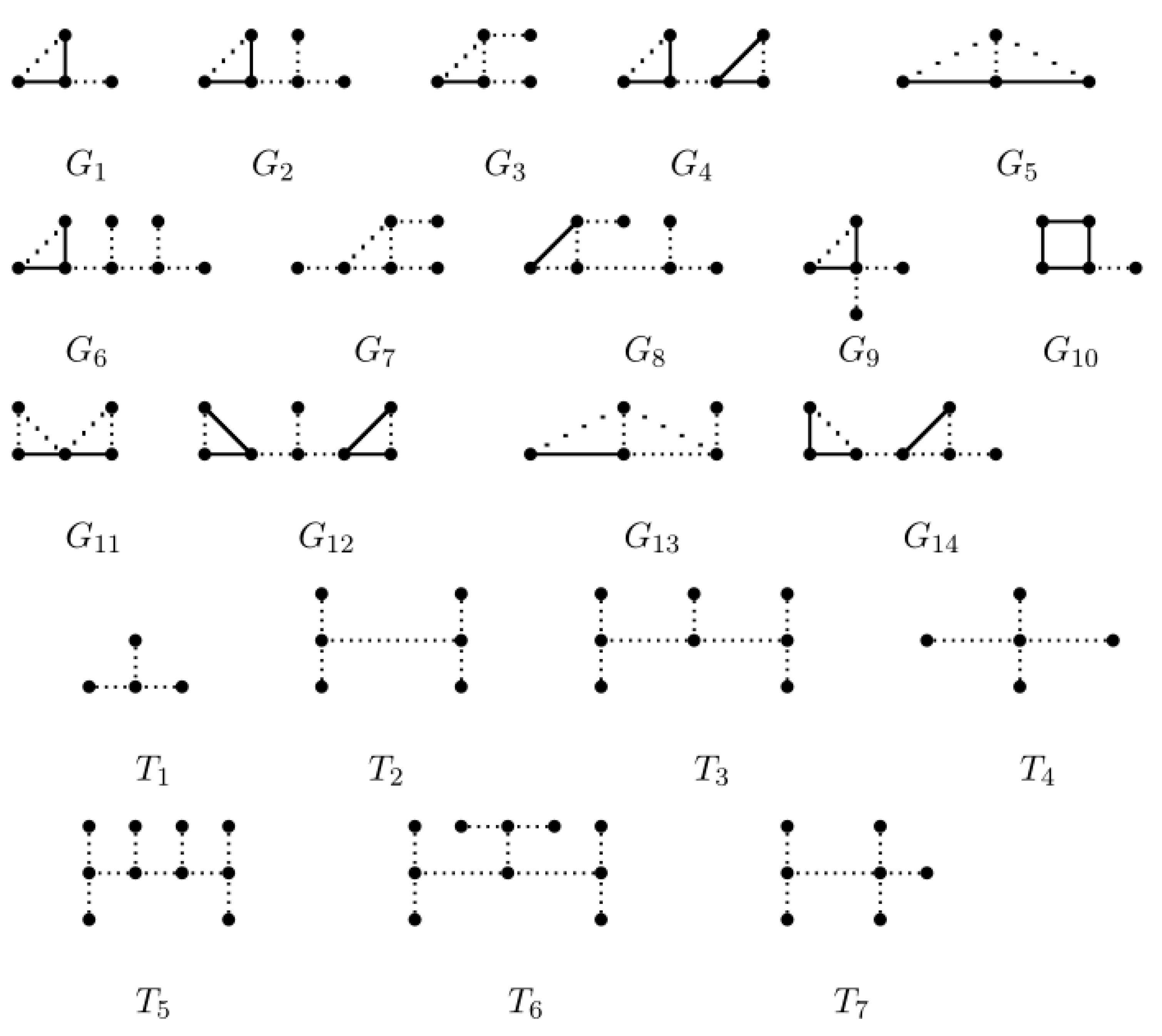
${\Pi }_1\left(G\right)=-3$ if and only if $G\in \{G_4,G_5,G_6,G_7,G_8,G_9,G_{10},T_5,T_6,T_7\}$, where all graphs are listed in Figure 1.

Note: $G_i$ in Figure 1, for $1\le i\le 14$ and $i\ne 10$, does not contain $C_4$ as its subgraphs and all the dot lines of the graphs denote a path with at least two vertices.

Now we give another invariant as follows:

Definition 2.

Let G be a connected graph. Set ${\Pi }_2\left(G\right)={\Pi }_1\left(G\right)+m\left(G\right)-n\left(G\right)$.

From Definitions 1 and 2 and Theorems 1–3, we can easily prove the following:  

Theorem 6. 

(1) Let G and H be two graphs such that $P_A(G,\lambda )=P_A(H,\lambda )$. Then

$${\Pi }_2\left(G\right)={\Pi }_2\left(H\right).$$

(2) Let G be a graph with k components $G_1,G_2,\cdots ,G_k$. Then

$${\Pi }_2\left(G\right)=\sum _{i=1}^k{\Pi }_2\left(G_i\right).$$

(3) Let G be a connected graph and $e\in E\left(G\right)$. Then

$${\Pi }_2\left(G\right)={\Pi }_2(G-e)-d_G\left(e\right)-2N_e\left(C_4\right)-N_e\left(C_3\right)+2.$$

Theorem 7.

Let G be a connected graph. Then, ${\Pi }_2\left(G\right)\le 0$, and the equality holds if and only if $G\in \mathcal{P}\cup \mathcal{C}\setminus \left\{C_4\right\}$.

Proof. 

By induction in $m\left(G\right)$, since ${\Pi }_2\left(K_1\right)=-1$ and ${\Pi }_2\left(K_2\right)=0$, we have (1) which holds when $m\left(G\right)\le 1$.

Suppose $m\left(G\right)\ge 2$. Choose $e\in E\left(G\right)$ such that ${(G-e)}_E$ is connected. Clearly, $d_G\left(e\right)\ge 1$. We distinguish the three following cases:

Case 1. e is a pendant edge.

Obviously, $G-e=H\cup K_1$, where $H={(G-e)}_E$. By Theorem 5 and the induction hypothesis, we have

$${\Pi }_2(G-e)={\Pi }_2\left(K_1\right)+{\Pi }_2\left(H\right)=-1+{\Pi }_2\left(H\right)$$

and

$${\Pi }_2\left(G\right)={\Pi }_2\left(H\right)-d_G\left(e\right)-2N_e\left(C_4\right)-N_e\left(C_3\right)+1\le {\Pi }_2\left(H\right)\le 0.$$

Note that ${\Pi }_2\left(G\right)=0$ if and only if ${\Pi }_2\left(H\right)=0,d_G\left(e\right)=1$ and $N_e\left(C_3\right)=N_e\left(C_4\right)=0$. By the induction hypothesis, $H\in \mathcal{P}\cup \mathcal{C}\setminus \left\{C_4\right\}$. Since $G-e=H\cup K_1$ and G is connected, we have $G\in \mathcal{P}$.

Case 2. e is an edge in a triangle.

We know that $G-e$ is connected and $N_e\left(C_3\right)\ge 1$. By Theorem 6 (3),

$${\Pi }_2\left(G\right)={\Pi }_2(G-e)-d_G\left(e\right)-2N_e\left(C_4\right)-N_e\left(C_3\right)+2\le {\Pi }_2(G-e)\le 0,$$

and ${\Pi }_2\left(G\right)=0$ if and only if ${\Pi }_2(G-e)=0,N_e\left(C_3\right)=d_G\left(e\right)=1$ and $N_e\left(C_4\right)=0$. By the induction hypothesis, $G-e\in \mathcal{P}\cup \mathcal{C}\setminus \left\{C_4\right\}$. Thus, $G\cong C_3$(only if $(G-e)\cong P_3$).

Case 3. e is an edge in a cycle whose length is greater than 3.

Clearly, $d_G\left(e\right)\ge 2$. By Theorem 6 (3), we have

$${\Pi }_2\left(G\right)={\Pi }_2(G-e)-d_G\left(e\right)-2N_e\left(C_4\right)-N_e\left(C_3\right)+2\le {\Pi }_2(G-e)\le 0$$

and ${\Pi }_2\left(G\right)=0$ if and only if ${\Pi }_2(G-e)=0,d_G\left(e\right)=2$ and $N_e\left(C_3\right)=N_e\left(C_4\right)=0$. By the induction hypothesis, $G-e\in \mathcal{P}\cup \mathcal{C}\setminus \left\{C_4\right\}$. Hence, $G\in \mathcal{C}\setminus \{C_3,C_4\}$.

Conversely, by Theorem 4 and Definition 2, we can directly verify our findings.   □

Let ${\Theta }_i=\left\{G\right|G$ be a connected graph and ${\Pi }_2\left(G\right)=i\}$. Similarly to ${\Pi }_1\left(G\right)$, we construct all connected graphs in ${\Theta }_i$ by the following algorithm.

Lemma 7.

Algorithm 2 is completeness, that is, if G is any connected graph with ${\Pi }_2\left(G\right)=i$ and $i\le 0$, then $G\in {\Theta }_i$ by Algorithm 2.

Proof. 

By induction in ${\Pi }_2\left(G\right)$ and $m\left(G\right)$. By Theorem 7, it is true for ${\Pi }_2\left(G\right)=0$. Suppose that the algorithm is completeness for ${\Pi }_2\left(G\right)>i$. When ${\Pi }_2\left(G\right)=i$, we shall prove the completeness by induction in $m\left(G\right)$.

By the proof of Theorem 7, we have that it is true for $m\left(G\right)\le 1$. Suppose that $m\left(G\right)\ge 2$, and we consider the following cases:

Case 1. G has a pendant edge, say $e=uv$ and $d_G\left(v\right)=1$. Then, $G-e=H\cup K_1$, where H is connected. Note that $N_e\left(C_3\right)+2N_{uv}\left(C_4\right)=0$. By the proof of case 1 of Theorem 7, we have

$${\Pi }_2\left(G\right)={\Pi }_2\left(H\right)-d_G\left(e\right)+1\le {\Pi }_2\left(H\right).$$

If $d_G\left(e\right)=1$, then ${\Pi }_2\left(H\right)=i$ and $m\left(H\right)=m\left(G\right)-1$, so by the induction hypothesis on $m\left(G\right)$, $H\in {\Theta }_i$. If $d_G\left(e\right)\ge 2$, then ${\Pi }_2\left(H\right)>i$, say ${\Pi }_2\left(H\right)=l>i$, and so $H\in {\Theta }_l$ by the induction hypothesis on ${\Pi }_2\left(G\right)$. Hence, G must be obtained from H by adding the pendant edge $uv$ from Algorithm 2, where $v\notin V\left(H\right)$.

Case 2. G has no any pendant edge. Then, there exists at least an edge $e=uv$ such that $H=G-uv$ is connected. Since $d_G\left(uv\right)+N_e\left(C_3\right)+2N_{uv}\left(C_4\right)\ge 2$, by Theorem 6 (3) we have

$${\Pi }_2\left(G\right)={\Pi }_2\left(H\right)-d_G\left(uv\right)-N_{uv}\left(C_3\right)-2N_{uv}\left(C_4\right)+2\le {\Pi }_2\left(H\right).$$

If $d_G\left(uv\right)+N_e\left(C_3\right)+2N_{uv}\left(C_4\right)=2$, then ${\Pi }_2\left(H\right)=i$ and $m\left(H\right)=m\left(G\right)-1$, so by the induction hypothesis on $m\left(G\right)$, $H\in {\Theta }_i$. If $d_G\left(uv\right)+N_e\left(C_3\right)+2N_{uv}\left(C_4\right)>2$, then ${\Pi }_2\left(H\right)>i$, say ${\Pi }_2\left(H\right)=l>i$, and so $H\in {\Theta }_l$ by the induction hypothesis on ${\Pi }_2\left(G\right)$. Hence, G must be obtained from H by adding the edge $uv$ from Algorithm 2. This completes the proof of the completeness.    □

Algorithm 2: Construction of all connected graphs with ${\Pi }_2\left(G\right)=i$.

(i) Take ${\Theta }_0=\left\{P_n\right|n\ge 2\}\cup \left\{C_3\right\}\cup \left\{C_n\right|n\ge 5\}$ and ${\Theta }_{-1}=\left\{K_1\right\}$. (ii) Let i be a negative integer, $i\le 0$, for $k:=0$ to i (step −1)  for each $H\in {\Theta }_k$   for each $u,v\in V\left(H\right),uv\notin E\left(H\right)$    if $N_H\left(uv\right)=k-i-N_{uv}\left(C_3\right)-2N_{uv}\left(C_4\right)+2$    then ${\Theta }_i:={\Theta }_i\cup \{H+uv\}$   end for   for each $u\in V\left(H\right)$    if $d_H\left(u\right)=k-i+1$    then ${\Theta }_i:={\Theta }_i\cup \{H+uv\}$, where $v\notin V\left(H\right)$.   end for  end for end for Note. In the front steps, $N_{uv}\left(C_3\right)$ (respectively, $N_{uv}\left(C_4\right))$ denotes the number of triangles (respectively, $C_4$) containing the edge $uv$ in the graph $H+uv$.

From Lemma 7, Theorems 6 and 7 as well as Algorithm 2, we can prove the following. Here, the proof is omitted.

Theorem 8.

Let G be a connected graph. Then:

(1) 

${\Pi }_2\left(G\right)=-1$ if and only if $G\in \{K_1,G_1,T_1\};$

(2) 

${\Pi }_2\left(G\right)=-2$ if and only if $G\in \{G_2,G_3,G_4,G_5,C_4,T_2\};$

(3) 

${\Pi }_2\left(G\right)=-3$ if and only if $G\in \{G_i,for6\le i\le 14,T_3,T_4\}$, where $G_i$, for $1\le i\le 14$ and $i\ne 10$, does not contain $C_4$ as its subgraph.

Remark 1.

The invariants ${\Pi }_1\left(G\right)$ and ${\Pi }_2\left(G\right)$ are important for determining DS graphs. By Theorems 6 and 7, for each component $G_i$ of the cospectral graphs of G, we have that ${\Pi }_2\left(G_i\right)\ge {\Pi }_2\left(G\right)$, which gives all possible cospectral graphs of G. It is therefore easy to find all possible cospectral graphs of G. Then, by considering the invariants ${\Pi }_1\left(G\right)$ and ${\Pi }_2\left(G\right)$, it can be ascertained whether G is determined by its adjacency spectrum.

Remark 2.

By Algorithms 1 and 2, one can characterize all connected graphs with ${\Pi }_1\left(G\right)<-k$ and ${\Pi }_2\left(G\right)<-k$. For example, $k=4,5$. Since there are many classes of graphs with ${\Pi }_1\left(G\right)=-k$ and ${\Pi }_2\left(G\right)=-k$ for a large positive integer k, it is difficult to characterize all graphs with ${\Pi }_1\left(G\right)=-k$ and ${\Pi }_2\left(G\right)=-k$.

Remark 3.

In this section, we define two invariants for graph G, which satisfies two important properties: component additivity (Theorems 2 and 6 (2)) and boundedness (Theorems 4 and 7). In fact, we define some new invariants with component additivity and boundedness. For example, ${\Pi }_3\left(G\right)={\pi }_1\left(G\right)+N_G\left(K_3\right)$ and ${\Pi }_4\left(G\right)={\pi }_2\left(G\right)+m\left(G\right)-n\left(G\right)$, which have similar properties and applications of ${\Pi }_1\left(G\right)$ and ${\Pi }_2\left(G\right)$. The readers interested by new invariants may study their properties and find more than DS graphs.

4. Some Graphs Determined by Their Adjacency Spectrum

For convenience, we denote by ${\mathcal{G}}_i$ the set $\left\{G_i\right\}$, for $1\le i\le 14$, and by ${\mathcal{T}}_i$ the set $\left\{T_i\right\}$, for $1\le i\le 4$. In Section 1, we list nearly all connected graphs G determined by their adjacency spectrum, which ${\Pi }_2\left(G\right)\in \{0,-1,-2\}$, except for $K_n$, $K_{m,m}$, $\overline{P_n}$ and $\overline{C_n}$. In fact, the necessary and sufficient conditions for all connected G with ${\Pi }_2\left(G\right)=0,-1$ to be DS were found. However, there are a few results on the DS-graphs of the connected graphs G with ${\Pi }_2\left(G\right)\le -2$, which are some special classes in ${\mathcal{G}}_3$, ${\mathcal{G}}_4$ and ${\mathcal{T}}_2$, seeing [9,15,16,26]. In this section, by using the results of previous sections, we shall give the necessary and sufficient conditions for one class of trees T with ${\Pi }_2\left(T\right)=-3$ and one class of graphs G with ${\Pi }_2\left(G\right)=-2$ to be DS with respect to their adjacency spectrum. In the following text, we use $P_A\left(G\right)$ instead of $P_A(G,\lambda )$.

Lemma 8

([27]). All roots of $P_A\left(C_n\right)$ and $P_A\left(P_n\right)$ are the following:

• $P_A\left(C_n\right):2cos\frac{2i\pi }{n},i=0,1,\cdots ,n-1.$
• $P_A\left(P_n\right):2cos\frac{i\pi }{n+1},i=1,\cdots ,n.$

Let $\lambda =2cos\theta$, set $t^{1/2}=e^{i\theta }$, and then it is useful to write the characteristic polynomial of $C_n$ and $P_n$ in the following form:

(1) 

$P_A(C_n,t^{1/2}+t^{-1/2})=t^{n/2}+t^{-n/2}-2$,

(2) 

$P_A(P_n,t^{1/2}+t^{-1/2})=t^{-n/2}(t^{n+1}-1)/(t-1)$.

The following graphs and lemmas are frequently used in following text.

Remark 4.

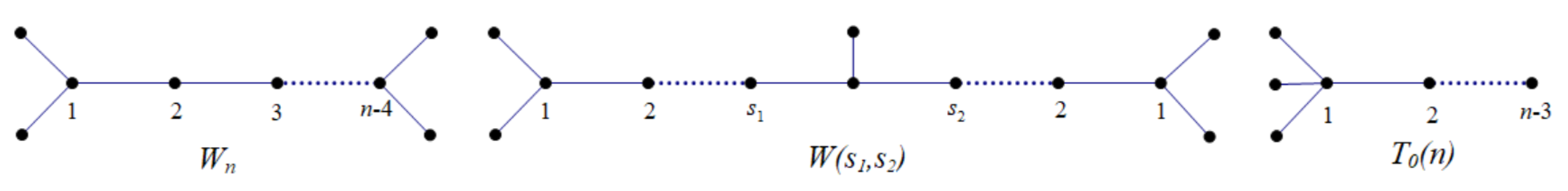
The parameters of each graph in Figure 2 take the following values: $n\ge 6$ for $W_n$, $s_2\ge s_1\ge 2$ for $W(s_1,s_2)$ and $n\ge 6$ for $T_0\left(n\right)$.

Lemma 9

([27]). (1) Let H be a proper subgraph of a connected graph G, then

$${\lambda }_1\left(H\right)<{\lambda }_1\left(G\right).$$

(2) For a graph G of n vertices with $v\in V\left(G\right)$, let $H=G-v$, then

$${\lambda }_1\left(G\right)\ge {\lambda }_1\left(H\right)\ge {\lambda }_2\left(G\right)\ge {\lambda }_2\left(H\right)\ge \cdots \ge {\lambda }_{n-1}\left(H\right)\ge {\lambda }_n\left(G\right).$$

An internal path of G is a walk $v_0{v}_1\cdots v_k$ ($k\ge 1$) that the vertices $v_1$, $v_2$, ⋯, $v_k$ are distinct ($v_0,v_k$ do not need to distinct), $d_G\left(v_0\right)\ge 2$, $d_G\left(v_k\right)\ge 2$ and $d_G\left(v_i\right)=2$ for $0<i<k$ [27].

Lemma 10

([27]). Let G be a connected graph that is not isomorphic to $W_n$ and let $G_{uv}$ be the graph obtained from G by subdividing the edge $uv$ of G. If $uv$ lies on an internal path of G, then ${\lambda }_1\left(G_{uv}\right)<{\lambda }_1\left(G\right)$.

Lemma 11

([27]). (1) The connected graphs with index 2 are precisely the graphs below: $C_n(n\ge 3)$, $W_n(n\ge 6)$, $K_{1,4}$ and $T(a,b,c)$ for $(a,b,c)\in \left\{\right(2,2,2),(1,2,5),(1,3,3\left)\right\}$.

(2) The connected graphs with an index of less than 2 precisely include the following graphs: $P_n(n\ge 1)$ and $T(a,b,c)$ for $(a,b,c)\in \left\{\right(1,2,2),(1,2,3),(1,2,4\left)\right\}\cup \left\{\right(1,1,n\left)\right|n\ge 1\}$.

Woo and Neumaier in [29] gave the structure of graphs with $\sqrt{2+\sqrt{5}}<{\lambda }_1\left(G\right)\le \frac{3}{2}\sqrt{2}$. An open quipu is a tree G of maximum degree 3 such that all vertices of degree 3 lie on a path and a closed quipu is a connected graph G of maximum degree 3 such that all vertices of degree 3 lie on a circuit and no other circuit exists. The following result can be found in [29].

Lemma 12

([29]). Let G be a connected graph with $\sqrt{2+\sqrt{5}}<{\lambda }_1\left(G\right)\le \frac{3}{2}\sqrt{2}$. Then, $\Delta \left(G\right)\in \{3,4\}$, where $\Delta \left(G\right)$ denotes the maximum degree of G, and:

(1) 

If $\Delta \left(G\right)=3$, then G is an open quipu or a closed quipu.

(2) 

If $\Delta \left(G\right)=4$, then $G\cong T_0\left(n\right),n\ge 2.$

Note that if G is an open quipu or a closed quipu, then ${\lambda }_1\left(G\right)$ may not belong to the interval $(\sqrt{2+\sqrt{5}},\frac{3}{2}\sqrt{2}]$, as can be seen in [29]. For a connected G with ${\Pi }_2\left(G\right)\ge -3$ and $\sqrt{2+\sqrt{5}}<{\lambda }_1\left(G\right)\le \frac{3}{2}\sqrt{2}$, by Lemma 12 and Theorem 8, we have $G\in \{G_1,G_3,G_7$, $T_1,T_2,T_3,T_0\left(n\right)\}$. The inverse is not true. For example, ${\lambda }_1\left(D_4\right)\simeq 2.17>\frac{3}{2}\sqrt{2}$, where $D_4$ is the graph obtained by adding a pendent edge to $C_3$ and $D_4\in {\mathcal{G}}_1$. Now, we consider the spectral characterizations of two classes of trees T such that $\sqrt{2+\sqrt{5}}<{\lambda }_1\left(T\right)\le \frac{3}{2}\sqrt{2}$ and ${\Pi }_2\left(T\right)=-3$, that is $W(s_1,s_2)$ and $T_0\left(n\right)$, as can be seen in Figure 2.

Lemma 13.

Let T be a tree and H be a graph with $m\left(H\right)=m\left(T\right)$ and $n\left(H\right)=n\left(T\right)$. If ${\Pi }_1\left(H\right)={\Pi }_1\left(T\right)$ and H has no $C_k$ as its subgraph, $k=3,4$, then we have

$$|b_6\left(H\right)|-|b_6\left(T\right)|=\frac{1}{3}{\displaystyle \sum _{i\in V\left(H\right)}}{d}_i^3\left(H\right)-\frac{1}{3}{\displaystyle \sum _{i\in V\left(T\right)}}{d}_i^3\left(T\right)+{\displaystyle \sum _{ij\in E\left(H\right)}}{d}_i{d}_j-{\displaystyle \sum _{ij\in E\left(T\right)}}{d}_i{d}_j+2N_H\left(C_6\right).$$

In particular, if H and G have the same degree sequence, then

$$|b_6\left(H\right)|-|b_6\left(T\right)|={\displaystyle \sum _{ij\in E\left(H\right)}}{d}_i{d}_j-{\displaystyle \sum _{ij\in E\left(T\right)}}{d}_i{d}_j+2N_H\left(C_6\right).$$

Proof. 

Since $m\left(H\right)=m\left(T\right)$, $n\left(H\right)=n\left(T\right)$ and $N_H\left(C_3\right)=N_H\left(C_4\right)=0$, by Lemma 5, we have ${\displaystyle \sum _{i\in V\left(H\right)}}{d}_i^2={\displaystyle \sum _{i\in V\left(T\right)}}{d}_i^2$; thus, the result holds. □

Remark 5.

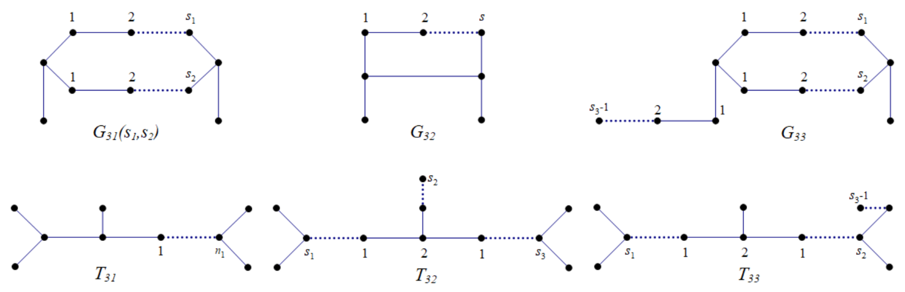
The parameters of each graph in Figure 3 take the following values: $s_2\ge s_1\ge 1$ for $G_{31}$, $s\ge 1$ for $G_{32}$, $s_2\ge s_1\ge 1$ and $s_3\ge 3$ for $G_{33}$, $n_1\ge 2$ for $T_{31}$, $s_3\ge s_1\ge 3$ and $s_2\ge 3$ for $T_{32}$, $s_1\ge 3$, $s_2\ge 3$ and $s_3\ge 3$ for $T_{33}$. Sometimes, we shall give the parameters of the graphs above, say, $G_{31}(n_1,n_2)$ in Lemma 4.9 and the proof of Theorem 4.1, which are $n_1$ and $n_2$ instead of the parameters $s_1$ and $s_2$ of $G_{31}$, respectively.

For a graph G with $uv\in E\left(G\right)$, $d_{\times }\left(uv\right)=d_G\left(u\right)\times d_G\left(v\right)$ is said to be the product degree of the edge $uv$. We denote by $D_{\times }\left(G\right)$ the sequence of the product degree of G, that is, $D_{\times }\left(G\right)=\{d_{\times }\left(e_1\right),d_{\times }\left(e_2\right),\cdots ,d_{\times }\left(e_m\right)\}$, where $E\left(G\right)=\{e_1,e_2,\cdots ,e_m\}$.

Lemma 14.

Let H be a graph with $m\left(H\right)=m\left(W(s_1,s_2)\right)$ and $n\left(H\right)=n\left(W(s_1,s_2)\right)$. Let ${\Pi }_i\left(H\right)={\Pi }_i(W(s_1,s_2)$, $i=1,2$, then we have:

(1) 

If $H=G_{31}\cup T(1,1,1)$, then $|b_6\left(H\right)|\ge |b_6\left(W(s_1,s_2)\right)|$, the equality holds if and only if H does not contain $C_6$ as its subgraph;

(2) 

If $H\in \{G_{31}\cup K_1,G_{31}\cup T(1,1,k),k\ge 2,G_{32}\cup T(1,1,1),G_{33}\cup T(1,1,1)\}$, then $|b_6\left(H\right)|\ge |b_6\left(W(s_1,s_2)\right)|+1$, the equality holds if and only if H does not contain $C_6$ as its subgraph;

(3) 

If $H=H_1\cup H_2$ and H is not a graph in (1) and (2), where $H_1\in {\mathcal{G}}_3\setminus \left\{G_{3i}\right|i=1,2,3\}$ and $H_2\in {\mathcal{T}}_1\cup \left\{K_1\right\}$, then $|b_6\left(H\right)|\ge |b_6\left(W(s_1,s_2)\right)|+2$;

(4) 

If $H=H_1\cup H_2$, where $H_1\in {\mathcal{G}}_7$ and $H_2\in \mathcal{P}$, then $|b_6\left(H\right)|\ge |b_6\left(W(s_1,s_2)\right)|+2$.

Proof. 

It is easy to see that each H of (1) and (2) and $W(s_1,s_2)$ have the same number of vertices and edges, as well as the same degree sequence. From Lemma 13, by direct computation, we see that (1) and (2) are true.

(3) Here, let $G_{3i}$, $i=1,2,3$, which do not contain $C_6$ as its subgraph. For each graph $F\in {\mathcal{G}}_3$, by Lemma 4.6 we have $|b_6\left(G_{32}\right)|=|b_6\left(G_{33}\right)|=|b_6\left(G_{31}\right)|+1$ and $|b_6\left(F\right)|>|b_6\left(G_{32}\right)|$ for all $F\in {\mathcal{G}}_3\setminus \left\{G_{3i}\right|i=1,2,3\}$, where $n\left(F\right)=n\left(G_{3i}\right)$, $i=1,2,3$. One can see that $|b_6\left(T(l_1,l_2,l_3)\right)|=|b_6\left(T(1,s_1,s_2)\right)|+1=|b_6\left(T(1,1,k)\right)|+2$ for $2\le l_1\le l_2\le l_3$, $2\le s_1\le s_2$ and $2\le k$, where $n\left(T(l_1,l_2,l_3)\right)=n\left(T(1,s_1,s_2)\right)=n\left(T(1,1,k)\right)$. Therefore, we have the following:

If $H_2=K_1$, it follows that $|b_6(F\cup K_1)|\ge |b_6(G_{31}\cup K_1)|+1$ for $F\in {\mathcal{G}}_3\setminus \left\{G_{31}\right\}$, which implies that (3) is true.

If $H_2=T(1,1,1)$, it follows that $|b_6(F\cup T(1,1,1))|\ge |b_6(G_{32}\cup T(1,1,1))|+1$ for $F\in {\mathcal{G}}_3\setminus \left\{G_{3i}\right|i=1,2,3\}$. By the (1) and (2) of the lemma, (3) holds.

If $H_2=T(1,1,k)$, $2\le k$, it follows that $|b_6(F\cup T(1,1,k))|\ge |b_6(G_{31}\cup T(1,1,k))|+1$ for $F\in {\mathcal{G}}_3\setminus \left\{G_{31}\right\}$. By (2) of the lemma, (3) holds.

If $H_2=T(1,s_1,s_2)$ with $2\le s_1\le s_2$, or $H_2=T(l_1,l_2,l_3)$ with $2\le l_1\le l_2\le l_3$, by the arguments above, we have that (3) holds.

(4) If $H_1\in {\mathcal{G}}_7$ and $H_2\in \mathcal{P}$ and $n(H_1\cup H_2)=n\left(W(s_1,s_2)\right)$, one sees that $H_1\cup H_2$ and $W(s_1,s_2)$ have the same number of edges, the same degree sequence, and the distinct product degree sequence. By the computation of the sum of the product degree, (4) follows from Lemma 13. □

Lemma 15.

Let $H\in {\mathcal{T}}_3$ and $n\left(H\right)=n\left(T_0\left(n\right)\right)=n$, then we have:

(1) 

If $H=W(s_1,s_2)$, then $|b_6\left(W(s_1,s_2)\right)|=|b_6\left(T_0\left(n\right)\right)|-1$, for $n\ge 10$;

(2) 

If $H\in \{T_{31},T_{32},T_{33}\}$, then $|b_6\left(H\right)|=|b_6\left(T_0\left(n\right)\right)|$, for $n\left(T_{31}\right)\ge 9$ and $n\left(T_{32}\right)=n\left(T_{33}\right)\ge 11$;

(3) 

If $H\in {\mathcal{T}}_3\setminus \{W(s_1,s_2),T_{1i}|i=1,2,3\}$, then $|b_6\left(H\right)|\ge |b_6\left(T_0\left(n\right)\right)|+1$.

Proof. 

Note that $s\ge 2$ for $T_{31}$, $3\le s_1\le s_3$ and $3\le s_2$ for $T_{32}$ and $3\le s_1$, $3\le s_2$ and $3\le s_3$ for $T_{33}$. By direct computation, (1) follows from Lemma 13.

For each $H\in {\mathcal{T}}_3$, by Lemma 13, we have that $|b_6\left(T_{31}\right)|=|b_6\left(T_{32}\right)|=|b_6\left(T_{33}\right)|=|b_6\left(W(s_1,s_2)\right)|+1$ and $|b_6\left(H\right)|\ge |b_6\left(W(s_1,s_2)\right)|+2$ for $H\in {\mathcal{T}}_3\setminus \{W(s_1,s_2),T_{1i}|i=1,2,3\}$. By lemma (1), it is easy to see that (2) and (3) hold. □

Lemma 16. 

(1) If $H=G_{31}(n_1,n_2)\cup T(1,1,1)$, then H and $W(s_1,s_2)$ are not cospectral, where $2\le s_1\le s_2$, $1\le n_1\le n_2$, $n=n\left(H\right)=n\left(W(s_1+s_2)\right)$.

(2) If $P_A\left(W(s_1,s_2)\right)=P_A\left(W(t_1,t_2)\right)$ with $2\le s_1\le s_2$ and $2\le t_1\le t_2$, then $s_1=t_1$ and $s_2=t_2$.

Proof. 

(1) Suppose that $W(s_1,s_2)$ and H are cospectral. Then, ${\Pi }_1\left(H\right)={\Pi }_1\left(W(s_1,s_2)\right)$, $|b_6\left(H\right)|=|b_6\left(W(s_1,s_2)\right)|$ and H does not contain odd circles as its subgraphs. By Theorem 5 and Lemma 14 (1), H does not contain $C_4$ and $C_6$ as its subgraphs, which implies that $n_1+n_2\ge 6$.

By Lemmas 1 and 2, the characteristic polynomials of $W(s_1,s_2)$ and H can be computed as follows:

$$\begin{array}{ccc}\hfill P_A\left(W(s_1,s_2)\right)& =& {\lambda }^3{P}_A\left(P_{s_1+s_2+3}\right)-2{\lambda }^3{P}_A\left(P_{s_1+s_2+1}\right)+{\lambda }^3{P}_A\left(P_{s_1+s_2-1}\right)-\hfill \\ & & {\lambda }^2{P}_A\left(P_{s_1+1}\right)P_A\left(P_{s_2+1}\right)+{\lambda }^2{P}_A\left(P_{s_1+1}\right)P_A\left(P_{s_2-1}\right)+\hfill \\ & & {\lambda }^2{P}_A\left(P_{s_1-1}\right)P_A\left(P_{s_2+1}\right)-{\lambda }^2{P}_A\left(P_{s_1-1}\right)P_A\left(P_{s_2-1}\right),\hfill \end{array}$$

$$P_A\left(H\right)=(\lambda P_A\left(P_3\right)-{\lambda }^2)({\lambda }^2{P}_A\left(C_{n_1+n_2+2}\right)-2\lambda P_A\left(P_{n_1+n_2+1}\right)+P_A\left(P_{n_1}\right)P_A\left(P_{n_2}\right)).$$

Since $n=s_1+s_2+6=n_1+n_2+8\ge 14$, by Lemma 4.1 and eliminating the same terms from $P_A(W(s_1,s_2),t^{1/2}+t^{-1/2})t^{\frac{s_1+s_2+6}{2}}{(t-1)}^2/{(t+1)}^2$ and $P_A(H,t^{1/2}+t^{-1/2})t^{\frac{n_1+n_2+8}{2}}{(t-1)}^2/{(t+1)}^2$, we can write (using Mathematica5.0) $P_A\left(W(s_1,s_2)\right)$ and $P_A\left(H\right)$, denoted by ${\varphi }_1$ and ${\varphi }_2$, as follows:

${\varphi }_1:-t^4-t^{2+s_1}+2t^{3+s_1}-t^{4+s_1}-t^{2+s_2}+2t^{3+s_2}-t^{4+s_2}-t^{2+s_1+s_2}$,

$$\begin{gathered} {\varphi }_2:-2t^4+t^5+t^6-t^{3+n_1}+t^{4+n_1}-t^{5+n_1}-2t^{1+n_1/2+n_2/2}+2t^{2+n_1/2+n_2/2} \\ +2t^{3+n_1/2+n_2/2}-4t^{4+n_1/2+n_2/2}+2t^{5+n_1/2+n_2/2}+2t^{6+n_1/2+n_2/2}-2t^{7+n_1/2+n_2/2}-t^{3+n_2}+ \\ {t}^{4+n_2}-t^{5+n_2}+t^{2+n_1+n_2}+t^{3+n_1+n_2}-2t^{4+n_1+n_2}. \end{gathered}$$

Now, we prove the necessity of lemma (1) by comparing the coefficients of the corresponding terms of ${\varphi }_1$ and ${\varphi }_2$.

Case 1. If $s_1=s_2$, we have ${\varphi }_1=-t^4-2t^{2+s_1}+4t^{3+s_1}-2t^{4+s_1}-t^{2+2s_1}$. Note that $s_1+s_2\ge 8$, and one sees $s_1=s_2\ge 4$. Then, the least term of ${\varphi }_1$ is $-t^4$ while the first term of ${\varphi }_2$ is $-2t^4$. Hence, other terms of the same exponents must exist in ${\varphi }_2$ such that the sum of the coefficients of which plus -2 equals -1. Since $n_1+n_2\ge 6$ and $n_2\ge n_1$, it is easy to see that all possible candidates are $-t^{3+n_1}$, or $-2t^{1+n_1/2+n_2/2}$. However, the least term of ${\varphi }_1$ and ${\varphi }_2$ are different, which is a contradiction.

Case 2. If $2=s_1<s_2$, substituting $s_1=2$ into ${\varphi }_1$ and by eliminating the same terms of ${\varphi }_1$ and ${\varphi }_2$, we have

${\varphi }_1^{\prime }:2t^5-t^6-t^{2+s_2}+2t^{3+s_2},$

$$\begin{gathered} {\varphi }_2^{\prime }:t^5+t^6-t^{3+n_1}+t^{4+n_1}-t^{5+n_1}-2t^{1+n_1/2+n_2/2}+2t^{2+n_1/2+n_2/2}+2t^{3+n_1/2+n_2/2} \\ -4t^{4+n_1/2+n_2/2}+2t^{5+n_1/2+n_2/2}+2t^{6+n_1/2+n_2/2}-2t^{7+n_1/2+n_2/2}-t^{3+n_2}+t^{4+n_2}-t^{5+n_2}+ \\ {t}^{2+n_1+n_2}+t^{3+n_1+n_2}. \end{gathered}$$

Note that $s_1+s_2\ge 8$ and $s_2\ge 6$. Clearly, the least term of ${\varphi }_1^{\prime }$ is $2t^5$. Therefore, other terms of the same exponents must exist in ${\varphi }_2^{\prime }$ such that the sum of the coefficients of which plus 1 equals 2. Since $n_1+n_2\ge 6$ and $n_2\ge n_1\ge 1$, it is not hard to see that all possible candidates are $-t^{3+n_1}$, $t^{4+n_1}$, $-2t^{1+n_1/2+n_2/2}$ and $2t^{2+n_1/2+n_2/2}$. All possible combinations of the terms are: $\{t^5,-t^{3+n_1},2t^{2+n_1/2+n_2/2}\}$, or $\{t^5,t^{4+n_1}\}$. For each combination above, we have that the least term of ${\varphi }_2^{\prime }$ is $-t^4$ and $-t^4$ does not vanish from ${\varphi }_2^{\prime }$, which is a contradiction.

Case 3. If $2<s_1<s_2$, the least term of ${\varphi }_1$ is $-t^4$. Since the first term of ${\varphi }_2$ is $-2t^4$, other terms of the same exponents must exist in ${\varphi }_2$ such that the sum of the coefficients of which plus -2 equals -1. Since $n_1+n_2\ge 6$ and $n_2\ge n_1\ge 1$, it is easy to see that all possible candidates are $-t^{3+n_1}$ and $-2t^{1+n_1/2+n_2/2}$. However, we combine the terms, the coefficient of which plus -2 is not -1, which completes the proof of (1).

(2) Since $s_1+s_2=t_1+t_2$, from ${\varphi }_1$, we get

$P_A\left(W(s_1,s_2)\right)$: $-t^{2+s_1}+2t^{3+s_1}-t^{4+s_1}-t^{2+s_2}+2t^{3+s_2}-t^{4+s_2}$,

$P_A\left(W(t_1,t_2)\right)$: $-t^{2+t_1}+2t^{3+t_1}-t^{4+t_1}-t^{2+t_2}+2t^{3+t_2}-t^{4+t_2}$.

Therefore, it follows that $s_1=t_1$ and $s_2=t_2$. □

Theorem 9.

Let $2\le s_1\le s_2$. Then, $W(s_1,s_2)$ is determined by its adjacency spectrum.

Proof. 

Let H be cospectral with $W(s_1,s_2)$. Suppose that H has k connected components $H_1$, $H_2$, ⋯, $H_k$. By Theorems 3.6–3.8, it is not hard to see that

$${\Pi }_2\left(H\right)=\sum _{i=1}^k{\Pi }_2\left(H_i\right)={\Pi }_2\left(W(s_1,s_2)\right)=-3.$$

By Theorem 7, ${\Pi }_2\left(H_i\right)\le 0$, therefore we have ${\Pi }_2\left(H_i\right)\ge -3$ for $1\le i\le k$. Choose the middle vertex v of degree 3 of $W(s_1,s_2)$ such that $W(s_1,s_2)-v=T(1,1,s_1)\cup T(1,1,s_2)\cup K_1$. By Lemma 11, ${\lambda }_1\left(T(1,1,n)\right)<2$. Thus, by Lemmas 9 and 12 (2), one can see that ${\lambda }_1\left(W(s_1,s_2)\right)>2$ and ${\lambda }_2\left(W(s_1,s_2)\right)<2$. On the other hand, it is easy to obtain that ${\lambda }_1\left(W_{2,2}\right)<\frac{3}{2}\sqrt{2}$. By Lemma 10, ${\lambda }_1\left(W(s_1,s_2)\right)<\frac{3}{2}\sqrt{2}$ for all $2\le s_1\le s_2$. Hence, we know that H only has one component, say $H_1$, such that $2<{\lambda }_1\left(H_1\right)\le \frac{3}{2}\sqrt{2}$ and ${\lambda }_1\left(H_i\right)<2$ for $2\le i\le k$. Note that ${\Pi }_2\left(H_i\right)\ge -3$, by Lemmas 11, 12 and Theorem 8, we have

$$H_1\in {\mathcal{G}}_1\cup {\mathcal{G}}_3\cup {\mathcal{G}}_7\cup {\mathcal{T}}_1\cup {\mathcal{T}}_2\cup {\mathcal{T}}_3\cup \left\{T_0\left(n\right)\right|n\ge 6\}$$

and for $i\ge 2$,

$$H_i\in \mathcal{P}\cup \left\{T(1,1,n)\right|n\ge 1\}\cup \left\{T(1,2,k)\right|k=2,3,4\}\cup \left\{K_1\right\}.$$

Clearly, $m\left(H_1\right)=n\left(H_1\right)$ for each $H_1\in {\mathcal{G}}_1\cup {\mathcal{G}}_3\cup {\mathcal{G}}_7$, $m\left(H_1\right)=n\left(H_1\right)-1$ for each $H_1\in {\mathcal{T}}_1\cup {\mathcal{T}}_2\cup {\mathcal{T}}_3\cup \left\{T_0\left(n\right)\right|n\ge 6\}$ and $m\left(H_i\right)=n\left(H_i\right)-1$ for each $i\ge 2$. Since $m\left(H\right)-n\left(H\right)=m\left(W(s_1,s_2)\right)-n\left(W(s_1,s_2)\right)=-1$, we have the following:

(i) $H=H_1\cup H_2$, where $H_1\in {\mathcal{G}}_1\cup {\mathcal{G}}_3\cup {\mathcal{G}}_7$ and $H_2\in \mathcal{P}\cup \left\{T(1,1,n)\right|n\ge 1\}\cup \left\{T(1,2,k)\right|k=2,3,4\}\cup \left\{K_1\right\}$; or

(ii) $H\in {\mathcal{T}}_1\cup {\mathcal{T}}_2\cup {\mathcal{T}}_3\cup \left\{T_0\left(n\right)\right|n\ge 6\}$.

Now we distinguish the following cases.

Case 1. $H_1\in {\mathcal{G}}_1$. By Theorems 4 and 5, ${\Pi }_1\left(H_1\right)=-1$ and ${\Pi }_1\left(H_2\right)\ge 0$. Then, by Theorem 2, ${\Pi }_1\left(H\right)\ge -1$, which contradicts ${\Pi }_1\left(H\right)={\Pi }_1\left(W(s_1,s_2)\right)=-2$.

Case 2. $H_1\in {\mathcal{G}}_3$. By Theorems 4 and 5, ${\Pi }_1\left(H_1\right)={\Pi }_1\left(W(s_1,s_2)\right)=-2$. By Theorems 2 and 4, ${\Pi }_1\left(H_2\right)=0$. By Lemma 14, we have that $|b_6\left(H\right)|=|b_6\left(W(s_1,s_2)\right)|$ if and only if $H=G_{31}(n_1,n_2)\cup T(1,1,1)$, where $G_{31}(n_1,n_2)$ does not contain $C_6$ as its subgraphs. From Lemma 16 (1), $P_A\left(H\right)\ne P_A\left(W(s_1,s_2)\right)$.

Case 3. $H_1\in {\mathcal{G}}_7$. By Theorems 4 and Theorem 5, ${\Pi }_1\left(H_1\right)=-3$. Since ${\Pi }_1\left(W(s_1,s_2)\right)=-2$, by Theorems 2 and 4, ${\Pi }_1\left(H_2\right)=1$, that is $H_2\cong P_t,t\ge 2$. By Lemma 14 (4), we have that $|b_6\left(H\right)|\ge |b_6\left(W(s_1,s_2)\right)|+2$, which implies that $P_A\left(H\right)\ne P_A\left(W(s_1,s_2)\right)$.

Case 4. H is a tree, that is $H\in {\mathcal{T}}_1\cup {\mathcal{T}}_2\cup {\mathcal{T}}_3\cup \left\{T_0\left(n\right)\right|n\ge 6\}$. By Theorem 3.5, ${\Pi }_1\left(H\right)={\Pi }_1\left(W(s_1,s_2)\right)=-2$. It therefore follows that $H\in {\mathcal{T}}_3\cup \left\{T_0\left(n\right)\right|n\ge 6\}$. By Lemma 15, $H=W_{t_1,t_2}$, where $t_1+t_2=s_1+s_2$. Therefore, $H=W(s_1,s_2)$ from Lemma 16 (2). We complete the proof of the theorem. □

From the proof of Theorem 4.1, we obtain a method to find DS graphs by the following steps.

(i) Characterize all connected graphs with ${\Pi }_1\left(G\right)=i$ and ${\Pi }_2\left(G\right)=j$, where $i\le 1$ and $j\le 0$.

(ii) For a given graph G, by applying the properties of invariants, such as ${\Pi }_1\left(G\right)$, ${\Pi }_2\left(G\right)$ and the number of triangles etc., we find all possible cospectral graphs of G.

(iii) Using the results of the eigenvalues, by considering the coefficients of the characteristic polynomial, we give a proof to whether G is determined by its adjacency spectrum.

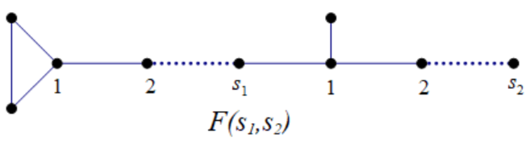
Here, we give an example to determine whether the graph $F(s_1,s_2)$ (as can be seen in Figure 4) is DS by using the above method.

Lemma 17

([21]). For a graph G, let $TrA{\left(G\right)}^k$ denote the trace of $A{\left(G\right)}^k$ ( or the number of close walks of length k in G), then:

(i) 

$Tr{A}^3=30N_G\left(K_3\right)$;

(ii) 

$Tr{A}^5=30N_G\left(K_3\right)+10N_G\left(C_5\right)+10N_G\left(D_4\right)$, where $D_4$ is the graph obtained from $K_3$ by adding an edge.

Suppose that H and $F=F(s_1,s_2)$ are cospectral. At first, we give some invariants. From Lemmas 2, 11 and 17 and Theorems 1 and 6, one can obtain the following invariants.

(i) H and F have the same number of vertices, edges and triangles.

(ii) $N_H\left(D_4\right)+N_H\left(C_5\right)=N_F\left(D_4\right)$.

(iii) ${\Pi }_i\left(H\right)={\Pi }_i\left(F\right)$, $i=1,2$.

(iv) Two is an eigenvalue of F if and only if $(s_1,s_2)\in \{(4,3),((6,2),(3,5)\}$.

Then, by using some properties (Theorems 3.2–3.8) of ${\Pi }_i(i=1,2)$ and the invariants above one give all possible cospectral graphs of F. Note that ${\Pi }_2\left(H\right)={\Pi }_2\left(F\right)=-2$, for $(s_1,s_2)\notin \{(4,3),(6,2),(3,5)\}$, we have

$$H\in \{G_{11}\cup G_{12}|G_{11},G_{12}\in {\mathcal{G}}_1\}\cup \left\{G_2\right|G_2\in {\mathcal{G}}_2\}\cup \{G_4\cup P_{n_i}|G_4\in {\mathcal{G}}_4,n_i\ge 2\}.$$

Finally, using the properties of the eigenvalues (Lemmas 9–11), by considering coefficients of the characteristic polynomial (Lemmas 5 and 8), one can determine the cospectral graphs of F.

From Lemmas 9 and 10, it is not hard to see that ${\lambda }_1\left(F\right)>{\lambda }_1\left(G_1\right)$ for all $G_1\in {\mathcal{G}}_1$. By Lemma 5, we have $b_6(G_4\cup P_{n_i})\ge b_6\left(F\right)+1$ for all $G_4\in {\mathcal{G}}_4,n_i\ge 2$ and $b_6\left(H\right)=b_6\left(F\right)$ for $H\in \left\{G_2\right|G_2\in {\mathcal{G}}_2\}$ if and only if $H=F(t_1,t_2)$, where $t_1+t_2=s_1+s_2$. Hence, H must be $F(t_1,t_2)$ with $t_1+t_2=s_1+s_2$. Let $t_1>s_1$ and $t_2<s_2$, by Lemmas 9 and 10, and it follows that ${\lambda }_1\left(F(s_1,s_2)\right)>{\lambda }_1\left(F(s_1,t_2)\right)>{\lambda }_1\left(F(t_1,t_2)\right)$, which implies $H=F(s_1,s_2)$.

When $(s_1,s_2)\in \{(4,3),((6,2),(3,5)\}$, by direct computation, we have that $F(s_1,s_2)$ is DS. Therefore, we obtain the following result.

Theorem 10.

 Let $s_1\ge 2$ and $s_2\ge 2$. Then, $F(s_1,s_2)$ is determined by its adjacency spectrum.

5. Conclusions

In this paper, at first, we gave two invariants ${\Pi }_1\left(G\right)$ and ${\Pi }_2\left(G\right)$ of G, obtained their properties and all connected graphs with ${\Pi }_1\left(G\right)\in \{1,0,-1,-2,-3\}$ and ${\Pi }_2\left(G\right)\in \{0,-1,-2,-3\}$. We then gave a method to characterize the graphs determined by their adjacency spectrum. To date, one can find the necessary and sufficient conditions for all G with ${\Pi }_2\left(G\right)\in \{0,-1\}$ to be determined by their adjacency spectrum, seeing [5,6,7,10,17]. For each graph G with ${\Pi }_2\left(G\right)=-2$, we find some DS graphs in the families ${\mathcal{G}}_4$ and ${\mathcal{G}}_5$ from [15,16,23,24,25,26] and some DS graphs in the family ${\mathcal{T}}_2$ from [9]. In this paper, we obtained two classes of DS graphs in the family ${\mathcal{G}}_2$ and ${\mathcal{T}}_3$. However, no other DS graphs in the family ${\mathcal{G}}_i$ were found, where $6\le i\le 14$ and $i\ne 10$. A natural follow up would be to characterize DS graphs in the families ${\mathcal{G}}_i$, where $6\le i\le 14$ and $i\notin \{10,11\}$. A more interesting avenue would be that of constructing a database of cospectral graphs by the above method and computation.

References

- Bondy, J.; Murty, U.S.R. Graph Theory; Springer: Berlin/Heidelberg, Germany, 2008. [Google Scholar]
- Schwenk, A.J. Almost all trees are cospectral. In New Directions in the Theory of Graphs; Academic Press: Cambridge, MA, USA, 1973; pp. 275–307. [Google Scholar]
- Godsil, C.G.; Mckay, B.D. Constructing cospectral graphs. Aequations Math. 1982, 25, 257–268. [Google Scholar] [CrossRef]
- Godsil, C.G. Algebra Combination; Academic Press: New York, NY, USA, 1980. [Google Scholar]
- Boulet, R.; Jouve, B. The Lollipop Graph is determined by its spectrum. Electron. J. Combin. 2008, 15, R74. [Google Scholar] [CrossRef]
- van Dam, E.R.; Haemers, W.H. Which graphs are determined by their spectrum? Linear Algebra Appl. 2003, 373, 241–272. [Google Scholar] [CrossRef] [Green Version]
- van Dam, E.R.; Haemers, W.H. Developments on spectral characterizations of graphs. Discrete Math. 2009, 309, 576–586. [Google Scholar] [CrossRef] [Green Version]
- Doob, M.; Haemers, W.H. The complement of the path is determined by its spectrum. Linear Algebra Appl. 2002, 356, 57–65. [Google Scholar] [CrossRef] [Green Version]
- Ghareghani, N.; Omidi, G.R.; Tayfeh-Rezaie, B. Spectral characterization of graphs with index at most . Linear Algebra Appl. 2007, 420, 483–489. [Google Scholar] [CrossRef] [Green Version]
- Haemers, W.H.; Liu, X.; Zhang, Y. Spectral characterizations of lollipop graphs. Linear Algebra Appl. 2008, 428, 2415–2423. [Google Scholar] [CrossRef] [Green Version]
- Haemers, W.H.; Spence, E. Enumeration of cospectral graphs. Eur. J. Comb. 2004, 25, 199–211. [Google Scholar] [CrossRef] [Green Version]
- Lu, P.; Liu, X.; Yuan, Z.; Yong, X. Spectral characterizations of sandglass graphs. Appl. Math. Lett. 2009, 22, 1225–1230. [Google Scholar] [CrossRef] [Green Version]
- Omidi, G.R. The spectral characterization of graphs of index less than 2 with no path as a component. Linear Algebra Appl. 2008, 428, 1696–1705. [Google Scholar] [CrossRef] [Green Version]
- Shen, X.; Hou, Y.; Zhang, Y. Graphs Zn and some graphs related to Zn are determined by their spectrum. Linear Algebra Appl. 2005, 404, 58–68. [Google Scholar] [CrossRef] [Green Version]
- Wang, J.; Huang, Q.; Belardo, F.; Marzic, E.M. On the spectral characterization of theta graphs, MATCH. Commun. Math. Comput. Chem. 2009, 62, 581–598. [Google Scholar]
- Wang, J.; Huang, Q.; Belardo, F.; Marzic, E.M. A note on the spectral characterization of dumbbell graphs. Linear Algebra Appl. 2009, 437, 1707–1714. [Google Scholar] [CrossRef] [Green Version]
- Wang, W.; Xu, C.X. On the spectral characterization of T-shape trees. Linear Algebra Appl. 2006, 414, 492–501. [Google Scholar] [CrossRef] [Green Version]
- Zhou, J.; Bu, C. Spectral characterization of line graphs of starlike trees. Linear Multilinear Algebra 2013, 61, 1041–1050. [Google Scholar] [CrossRef]
- Liu, X.; Zhang, Y.; Gui, X. The multi-fan graphs are determined by their Laplacian spectra. Discrete Math. 2008, 308, 4267–4271. [Google Scholar] [CrossRef]
- Omidi, G.R.; Tajbakhsh, K. Starlike trees are determined by their Laplacian spectrum. Linear Algebra Appl. 2007, 422, 654–658. [Google Scholar] [CrossRef] [Green Version]
- Omidi, G.R. On a Laplacian spectral characterization of graphs of index less than 2. Linear Algebra Appl. 2008, 429, 2724–2731. [Google Scholar] [CrossRef] [Green Version]
- Caḿara, M.; Haemers, W.H. Spectral characterizations of almost complete graphs. Discret. Appl. Math. 2014, 176, 19–23. [Google Scholar] [CrossRef]
- Liu, F.; Huang, Q.; Wang, J.; Liu, Q. The spectral characterization of ∞-graphs. Linear Algebra Appl. 2012, 437, 1482–1502. [Google Scholar] [CrossRef] [Green Version]
- Wang, J.; Belardo, F.; Huang, Q.; Marzic, E.M. Spectral characterizations of dumbbell graphs. Electron. J. Combin. 2010, 17, R42. [Google Scholar] [CrossRef]
- Wang, J.; Huang, Q.; Belardo, F.; Marzic, E.M. On the spectral characterizations of ∞-graphs. Discret. Math. 2010, 310, 1845–1855. [Google Scholar] [CrossRef] [Green Version]
- Ramezani, F.; Broojerdian, N.; Tayfeh-Rezaie, B. A note on the spectral characterization of θ-graphs. Linear Algebra Appl. 2009, 431, 626–632. [Google Scholar] [CrossRef] [Green Version]
- Cvetkovic, D.M.; Doob, M.; Sachs, H. Spectra of Graph; Academice Press: New York, NY, USA, 1980. [Google Scholar]
- Zhao, H.; Liu, R. On the character of the matching polynomial and its application to circuit characterization of graphs. JCMCC 2001, 37, 75–86. [Google Scholar]
- Woo, R.; Neumaier, A. On graphs whose spectral radius is bounded by . Graphs Combin. 2007, 23, 713–726. [Google Scholar] [CrossRef]
Figure 1.
Some connected graphs .
Figure 2.
Graphs , and .
Figure 3.
Some graphs in and .
Figure 4.
.
Publisher’s Note: MDPI stays neutral with regard to jurisdictional claims in published maps and institutional affiliations. |
© 2022 by the authors. Licensee MDPI, Basel, Switzerland. This article is an open access article distributed under the terms and conditions of the Creative Commons Attribution (CC BY) license (https://creativecommons.org/licenses/by/4.0/).
Share and Cite
MDPI and ACS Style
Yin, J.; Zhao, H.; Xie, S. Spectral Invariants and Their Application on Spectral Characterization of Graphs. Axioms 2022, 11, 260. https://0-doi-org.brum.beds.ac.uk/10.3390/axioms11060260
AMA Style
Yin J, Zhao H, Xie S. Spectral Invariants and Their Application on Spectral Characterization of Graphs. Axioms. 2022; 11(6):260. https://0-doi-org.brum.beds.ac.uk/10.3390/axioms11060260
Chicago/Turabian StyleYin, Jun, Haixing Zhao, and Sun Xie. 2022. "Spectral Invariants and Their Application on Spectral Characterization of Graphs" Axioms 11, no. 6: 260. https://0-doi-org.brum.beds.ac.uk/10.3390/axioms11060260
Note that from the first issue of 2016, this journal uses article numbers instead of page numbers. See further details here.