1. Introduction
In 1965, Zadeh [
1] was the first to establish the notion of an FS.
and
are the two degrees of measurement in an FS. An MD within the interval
defines the element of a set in
, whereas
can be generated by subtracting
from
. Following Zadeh, Atanassov [
2] improved this notion by suggesting the concept of the IFS, in which
and
are outlined independently but with the requirement that their total belongs to the scale
. Furthermore, the term
was characterized as a hesitancy degree (HD). There are certain limits in the Atanassov model of IFS, as the total of
and
frequently falls outside of the interval
. As a result, Yager [
3] introduced a new notion known as the PyFS, in which the area for assigning the MD and NMD of IFSs is expanded, and the requirement of the PyFS becomes
. However, this is not always applicable, as squaring the sum sometimes results in it falling outside of the unit interval
, showing the limitations of the PyFS. As a result, Yager [
4] proposed the idea of the q-ROFS, in which the sum of the q-th power of MD and the q-th power of NMD is equal to or less than 1. The q-ROFS condition becomes
.
Without a doubt, Atanassov’s model of IFSs improved Zadeh’s concept of FSs; however, there are occasions when more than two choices exist, whereby IFSs fail to describe and solve such problems. Cuong and Kreinovich [
5] proposed a novel model called the PFS, which includes three characteristic functions defined as
,
and
, where
is the abstinence degree (AD), with the requirement that their sum must fall within the interval
. The term
refers to the refusal degree (RD) of an element of the PFS. PFSs broadened the scope of FSs and IFSs; however, the problem still exists that we cannot assign the values of the MD, NMD, and AD. After realizing certain limitations that exist in the structures of FSs, IFSs, and PFSs, Mahmood et al. [
6] expanded this concept and presented the notion of the SFS as a modification of PFSs by extending their range. The sum of
,
and
may fall outside of the unit interval in the structure of SFSs, but their square must fall within the unit interval, which is specified as
. SFSs have a larger domain than PFSs due to their new condition. Sometimes, such a situation occurs where the total of the squares of
,
and
falls outside the unit interval, rendering this method insufficient. To cope with such situations, Mahmood et al. [
6] developed an extension of SFSs called the TSFS, which has no restrictions. The TSFS contains the constraint that
, where
. Considering the above-described research, it can be concluded that the TSFS is a modification of the IFS, PyFS, and PFS, with no limitations. TSFSs are more important than IFSs, PyFSs, and PFSs since they have greater space. As a result, in TSFSs, we can allocate the values of the MD, NMD, and AD to our liking due to the greater space available, which is infeasible in IFSs, PyFSs, and PFSs due to their constrained structure.
The DM is a tool for calculating the difference between distinct items on a scale of
, while the SM is a scheme that calculates the degree of similarity between two items on a scale of
. Several DMs and SMs have been introduced in various extended versions of FSs. Wang and Xin [
7] analyzed the links between the DMs and SMs of IFSs, and used their suggested DMs and SMs to recognize patterns. Xiao [
8] presented a DM for IFSs based on the Jenson–Shannon divergence and used it as an algorithm for pattern classification, thus providing a solution to the interference concerns. Jiang et al. [
9] suggested a DM and SM for IFSs based on a transformed isosceles triangle, using them to tackle pattern-recognition difficulties. Du and Hu [
10] presented aggregation DMs and the induced SMs of IFSs and successfully utilized them in a variety of pattern-recognition applications. DMs and SMs of PyFSs were suggested by Zeng et al. [
11] and applied to MCDM. They also presented a numerical example to test the suggested decision-making method’s efficacy. On the basis of the Hausdorff metric, Hussain and Yang [
12] presented the DMs and SMs of PyFSs. To test the validity of the suggested DMs and SMs, they were used to recognize several patterns based on linguistic variables. Wang et al. [
13] designed DMs and SMs of q-ROFSs using cosine functions and applied them to pattern-recognition and scheme-selection issues. Liu et al. [
14] suggested various cosine DMs and SMs of q-ROFSs and used them to tackle issues such as decision making from both a geometric and an algebraic perspective. Garg et al. [
15] suggested generalized Dice SMs of complicated q-ROFSs and used them to solve issues such as pattern recognition and medical diagnosis. Khan et al. [
16] suggested better cosine and cotangent function-based SMs of q-ROFSs and tested their validity using numerical examples. The notion of complex q-ROF variation coefficient SMs was presented by Liu et al. [
17], and the suggested SMs were used for medical diagnosis and pattern-recognition challenges. Donyatalab et al. [
18] presented DMs and SMs of q-ROFSs based on the square root cosine similarity measure and expanded them in two states: with and without HD. Khan et al. [
19] proposed bi-parametric DMs and SMs of PFSs and used them in medical diagnosis. Cosine SMs of PFSs were developed by Wei [
20], and the proposed SMs were applied to strategic decision-making issues. Wei [
21] introduced SMs of PFSs and offered examples to demonstrate their validity for building material recognition and mineral field recognition. Jan et al. [
22] presented a set of generalized DMs and SMs of PFSs and used them to tackle issues such as building material detection and MADM. Khan et al. [
23] introduced DMs and SMs of SFSs and used them to solve data mining, medical diagnosis, and MADM problems. Rafiq et al. [
24] presented cosine SMs of SFSs and used them to solve issues involving MADM. Wei et al. [
25] proposed certain SMs of SFSs based on cosine functions and used them to solve pattern-recognition and medical diagnosis problems. Shishavan et al. [
26] proposed various new SMs of SFSs and used them to solve problems such as medical diagnosis and green supplier selection. Wu et al. [
27] presented cosine-based SMs of TSFSs and used them for pattern-recognition issues. Ullah et al. [
28] proposed SMs of TSFSs and used them for pattern-recognition tasks. Abid et al. [
29] suggested a novel SM for TSFSs and discussed its applications in pattern recognition and decision making. Ibrahim et al. [
30] discussed (3,2)-fuzzy sets and suggested their applications to topology and optimal choices. Al-shami et al. [
31] suggested SR-fuzzy sets and discussed their applications to weighted aggregated operators in MADM.
Several SMs and DMs have been developed so far and discussed previously, such as the SMs suggested by Wang et al. [
13], Liu et al. [
14], Garg et al. [
15], Khan et al. [
16], Peng and Liu [
32], Zeng et al. [
33], and Zeng et al. [
34]. All of these studies discussed only two aspects of imprecise and uncertain information and hence led towards information loss. In the context of TSFSs, we develop several SMs and DMs that address four characteristics of information that are ambiguous and imprecise. In handling issues with ambiguous knowledge, these SMs and DMs provide higher accuracy, reliability, and fascinating flexibility. We draw a comparison between the proposed and past SMs and DMs to see how adaptive the proposed method is. We discuss all four degrees of TSFSs, i.e., MD, AD, NMD, and RD, demonstrating the novelty of this concept. Because all of these degrees are present, the spectrum of TSFSs expands, revealing the limitations of all previously described notions such as IFSs, PyFSs, q-ROFSs, and PFSs. Existing conceptions are unable to handle the difficulties when discussed in a TSF environment due to their limited range and lack of degrees. When data are provided in a TSF environment, the proposed DMs and SMs can solve any real-life difficulty by analyzing the facts. The significance of the topic stems from its concept, which demonstrates that the previously defined DMs and SMs failed to solve challenges when information was delivered in a TSF setting due to their limited range and low adaptability. As a result of the constraints of existing DMs and SMs, the suggested DMs and SMs can alleviate problems when data are presented in a TSF environment.
The remaining portion of the paper is arranged based on some definitions of TSFSs, as presented in
Section 2.
Section 3 and
Section 4 define new DMs and SMs, respectively.
Section 5 looks at some numerical examples and applications of presented DMs and SMs for developing an algorithm for pattern recognition and MCDM.
Section 6 discusses some of the current work’s consequences. Finally, in
Section 7, we present our conclusion.
3. Distance Measures for TSFSs
Here, we propose some DMs based on T-spherical fuzzy information. The proposed new DMs are supported by examples, and their exceptional cases are studied.
Definition 4. Let . A DM denoted by is a mapping of , possessing the features listed below:
- (1)
- (2)
- (3)
iff .
- (4)
.
- (5)
If then and
Theorem 1. Let . Then is a DM.
Proof of Theorem 1. We only give the proof of (2).
Suppose
i.e.,
Hence,
- (1)
Similarly, from (1).
- (2)
From the formula, we obtain
Because , so . Hence,
- (3)
Similarly, from (5).
- (4)
From the formula, we obtain
Because
So . Likewise, . □
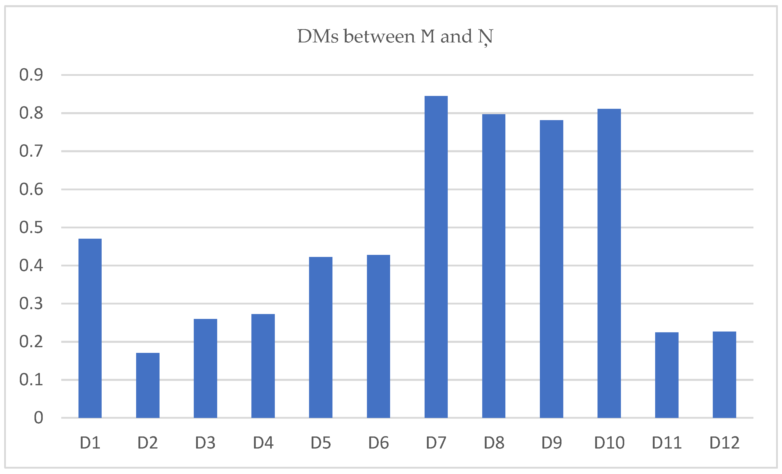
Example 1. Let as given in Table 1. Bothandare TSFSs for.
We applied the DMs
defined above to the two sets provided in
Table 1, and the outcomes are portrayed in
Table 2.
6. Algorithm and Applications
This section aims to check the effectiveness of the presented DMs and SMs. For this purpose, we design an algorithm for pattern recognition to check which pattern is useful. Moreover, we provide some applications of the newly introduced DMs and SMs in MADM to check which is the best selection for MADM while using the newly introduced DMs and SMs.
6.1. Algorithm in Pattern Recognition
Let be a finite parameter; there are m patterns and a test sample . To check the closeness, we ask to which pattern does the sample belong to? The recognition steps are listed below:
Step 1. First, we have to evaluate the DM and SMs between and , respectively.
Step 2. Then, we have to select the minimum from and maximum from , respectively, i.e., and . Then, the test sample is classified into pattern according to the principle of the minimum of DMs and maximum of SMs.
Example 6.1. We use the DMs and SMs given in this research to tackle the challenge of recognizing construction materials presented by Ullah et al. [
28]. Let us assume TSFNs
which show building materials of four types. Let us consider
as the attributes. There is another unknown material
. Using some DMs and SMs defined for TSFSs, we will define the class from four materials of unknown material denoted by
. Then, we have to evaluate class
to
.
Step 1. All the information provided in
Table 5 is about the type of TSFNs. It is worth noting that all of the numbers in
Table 5 are TSFNs for
, signaling that neither IFS nor PFS methods can handle this type of data.
Step 2. The DM of each TSFN given in
Table 5 is evaluated with
using the newly defined DMs in
Section 3.
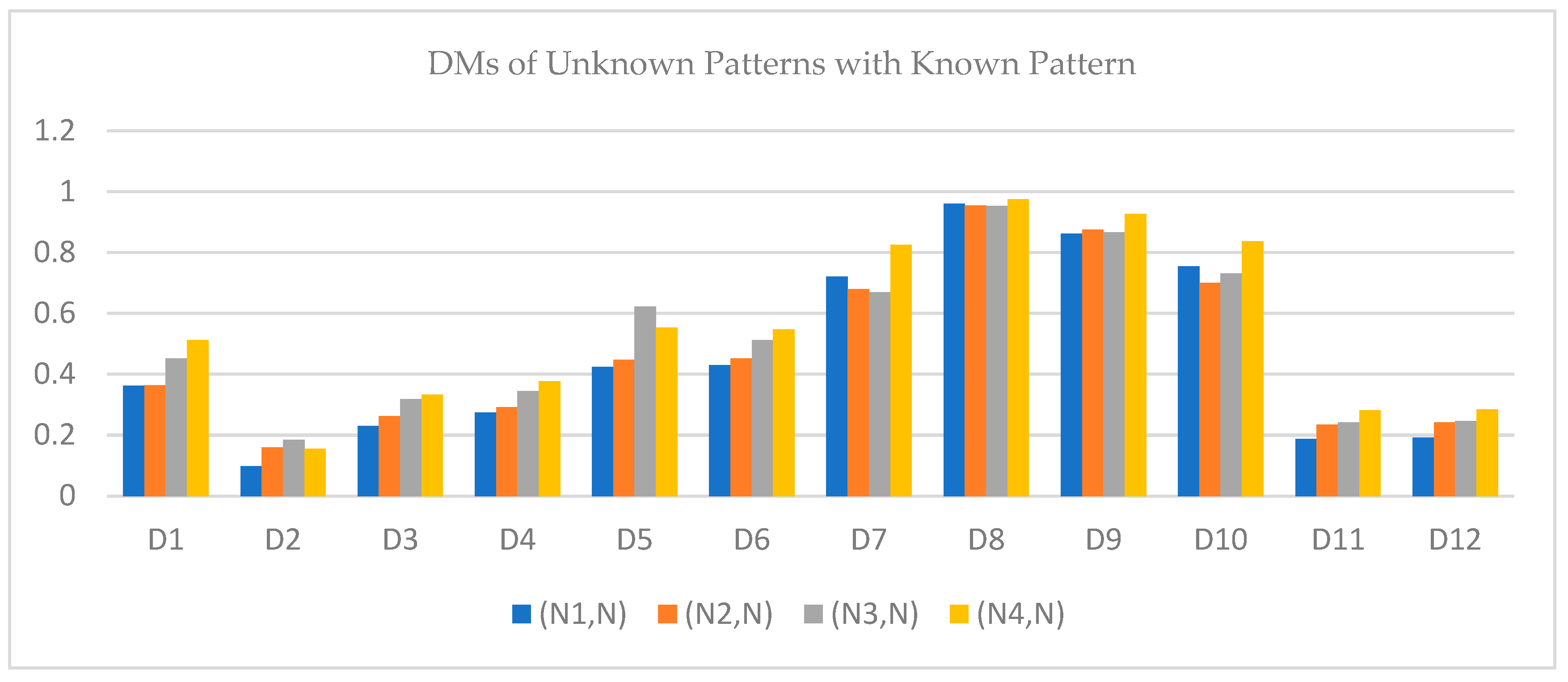
Step 3. Examining
Table 6, for DMs the result obtained is
Hence, the pattern is closer to as the DM of is smaller than all the remaining pairs. Therefore, it is said that the unknown pattern belongs to an -type pattern.
The results obtained in
Table 6 are shown in
Figure 3 below, which indicates that the distance of the unknown pattern
is closer to
.
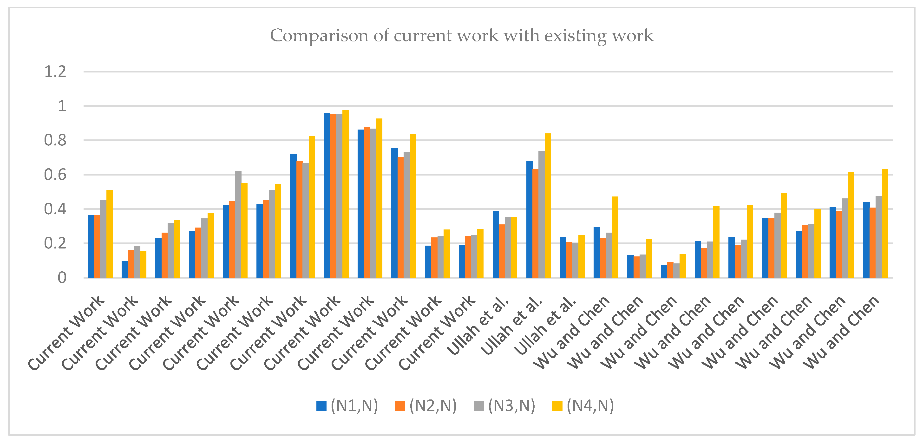
Comparative Study: This section aims to compare the results achieved using DM for TSFSs in the current work with results obtained using DM for TSFSs, as proposed by Ullah et al. [
28] and Wu and Chen [
27]. Here, we also present the limitations of the previously defined DMs of IFSs and PFSs. A brief discussion of the calculated results of this paper compared with other papers is given in
Table 7 below.
The results shown in
Table 7 support our hypothesis that the DM of TSFSs can manage large amounts of data. The benefit of the introduced DMs is that there are no restrictions on giving values to membership degrees in the environment of TSFSs as it includes all four degrees. There are restrictions when assigning values to membership degrees in IFSs, PyFSs, and PFSs. All the existing DMs failed to solve the issues due to the absence of RD and the restricted range when the data are given in the TSF environment. It is also concluded from
Table 8 that
is close to
as the distance of
is smaller than all the remaining pairs. Therefore, it is concluded that the unknown pattern
belongs to an
-type pattern, which supports our results.
Figure 4 depicts a comparison of our work with that of others, and explains that our results are more convenient and accurate than those of previous work.
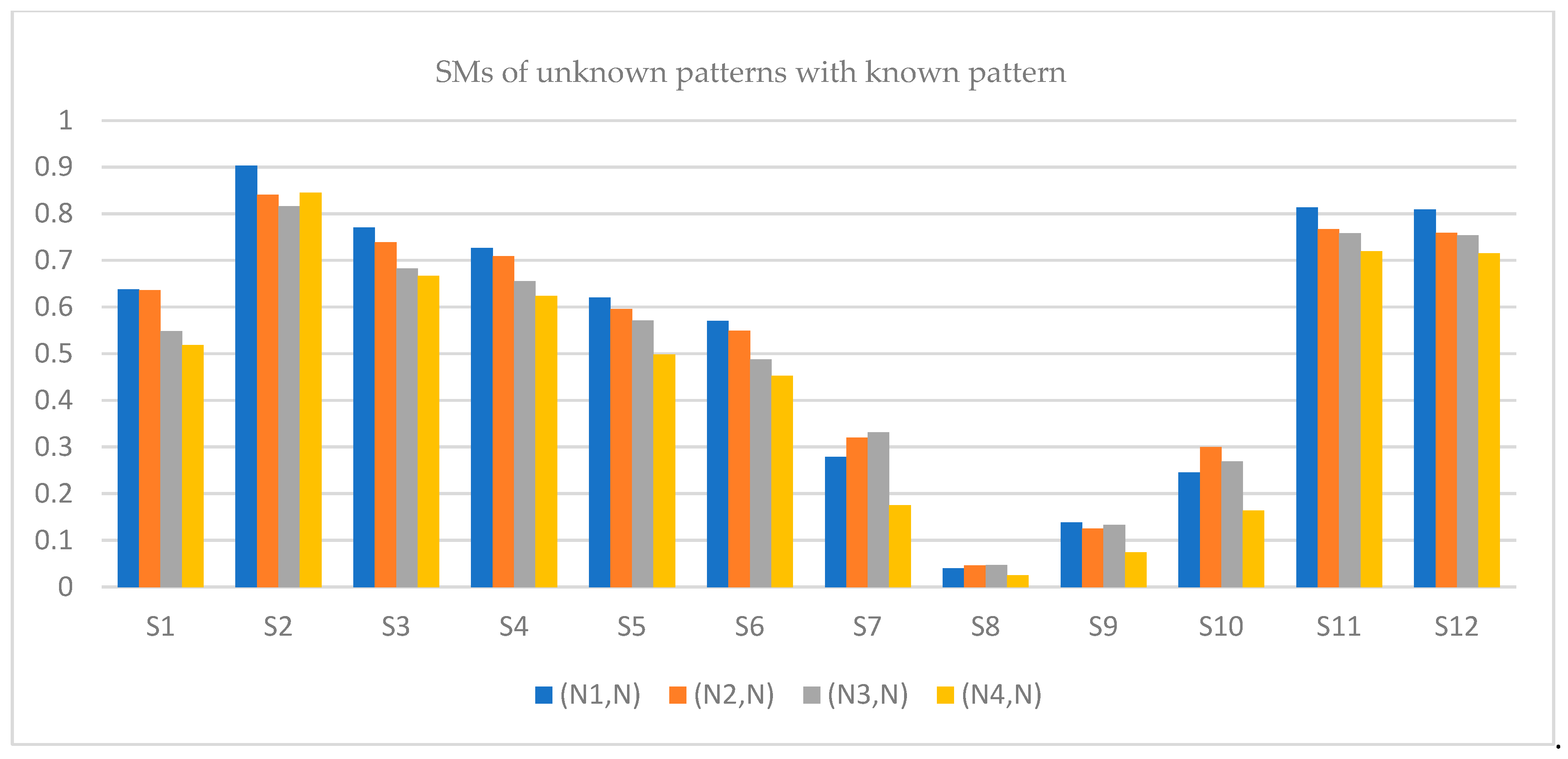
The SM of each TSFN given in
Table 5 is evaluated with
using the newly defined SMs in
Section 4.
Examining
Table 8, for SMs the result obtained is
Hence, the pattern is close to , as the SM of is greater than all the remaining pairs. Therefore, it is said that the unknown pattern belongs to an -type pattern.
The results obtained in
Table 8 are shown in
Figure 5 below, which indicates that the similarity of the unknown pattern
is close to
.
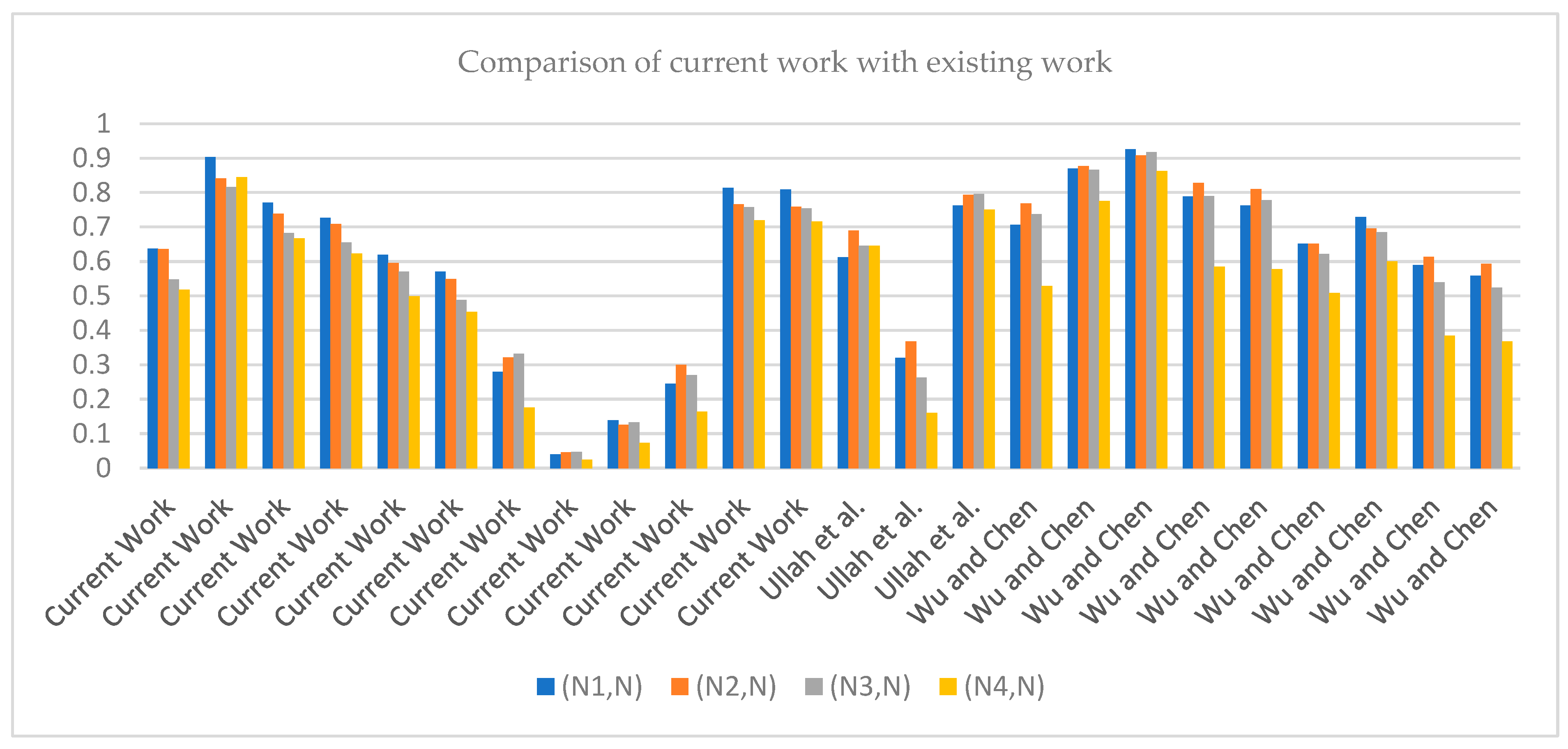
Comparative Study: This section aims to compare the results achieved using SM for TSFSs in the current work with results obtained using SM for TSFs, as proposed by Ullah et al. [
28] and Wu and Chen [
27]. Here, we also present the restrictions of the previously defined SMs of IFSs and PFSs. A brief discussion of the calculated results of this paper compared with other papers is given in
Table 9 below.
The results in
Table 9 support our hypothesis that the SM of TSFSs can manage large amounts of data. The benefit of the introduced SMs is that there are no restrictions on giving values to membership degrees in the environment of TSFSs as it includes all four degrees, but there are restrictions on assigning values to membership degrees in IFSs, PyFSs, and PFSs. All existing SMs failed to solve the issues due to the absence of RD and the restricted range, especially when the data are given in the environment of TSFSs. It is also concluded from
Table 9 that
is close to
as the similarity of
is more significant than all the remaining pairs. Therefore, it is said that the unknown pattern
belongs to an
-type pattern, which supports our results.
Figure 6 depicts a comparison of our work with that of others and also explains that our results are suitable and more accurate than those of previous work.
6.2. Applications in MCDM
Here, we will present the applications of the introduced DMs and SMs for MCDM.
Example 6.2. We use the DMs and SMs given in this research to tackle the challenge of MCDM presented by Ullah et al. [
35]. Islamabad, Pakistan’s capital, is regarded as one of the world’s most beautiful cities. A large number of people regularly frequent Islamabad’s parks and picnic areas. The Metropolitan Corporation of Islamabad (MCI), is in charge of the city’s administration. To maintain its appeal, the MCI decided to refurbish all of the parks and picnic areas. The MCI needed to recruit some private contractors to do so. The MCI chose four private companies for further consideration after some preliminary screening.
: Bilawal Builders,
: Hussain Estate and Builders,
: Nimo Engineering, Construction and Interiors, and
: Scholar Builders. The MCI’s specialists devised five-point criteria for selecting the best corporation or company:
: cost,
: previous performance,
: time constraints,
: quality assurance, and
: labor quantity. The decision-making committee provided all of the information regarding TSFNs, which is given in
Table 10. The evaluation steps for the MCDM algorithm are given as:
Step 1. Table 10 contains the decision maker’s suggestions in the form of TSFNs. Assuming that all of the values in
Table 10 are simply TSFNs for
, it is demonstrated that neither IFS nor PFS operators can solve this problem.
Step 2. The DM of each TSFN given in
Table 10 is calculated with
, which describes an ideal TSFN using newly introduced DMs, as shown in
Section 3.
Step 3. Analyzing
Table 11, for DMs the result obtained is
Therefore, is the best choice as the DM of is smaller than all the remaining pairs. Furthermore, due to the complex nature of TSFNs, the DMs of IFSs and PFSs cannot be applied to this sort of data.
The outcomes of
Table 11 are portrayed in
Figure 7, which shows that after applying the proposed DMs,
is the best choice for MCDM purposes.
Comparative Study: This section aims to compare the results achieved using DM for TSFSs in the current work with results obtained using DM for TSFs, as proposed by Ullah et al. [
28]. Here, we also present the limitations of the previously defined DMs of IFSs and PFSs. A brief discussion of the calculated results of this paper compared with other papers is given in
Table 12 below.
The results in
Table 12 support our hypothesis that the DM of TSFSs can manage large amounts of data. The benefit of the introduced DMs is that there are no restrictions on giving values to membership degrees in the environment of TSFSs as it includes all four degrees, but there are restrictions on giving values to membership degrees in IFSs, PyFSs, and PFSs. All the existing DMs failed to solve the issues due to the absence of RD and the restricted range when the data are given in the TSF environment. It is also concluded from
Table 13 that
is the best choice as the DM of
is smaller than all the remaining pairs. Therefore, it is said that
is the best choice for MCDM purposes, which supports our results.
Figure 8 depicts a comparison of our study with others, and it also explains that our results are suitable and more accurate than those of previous work.
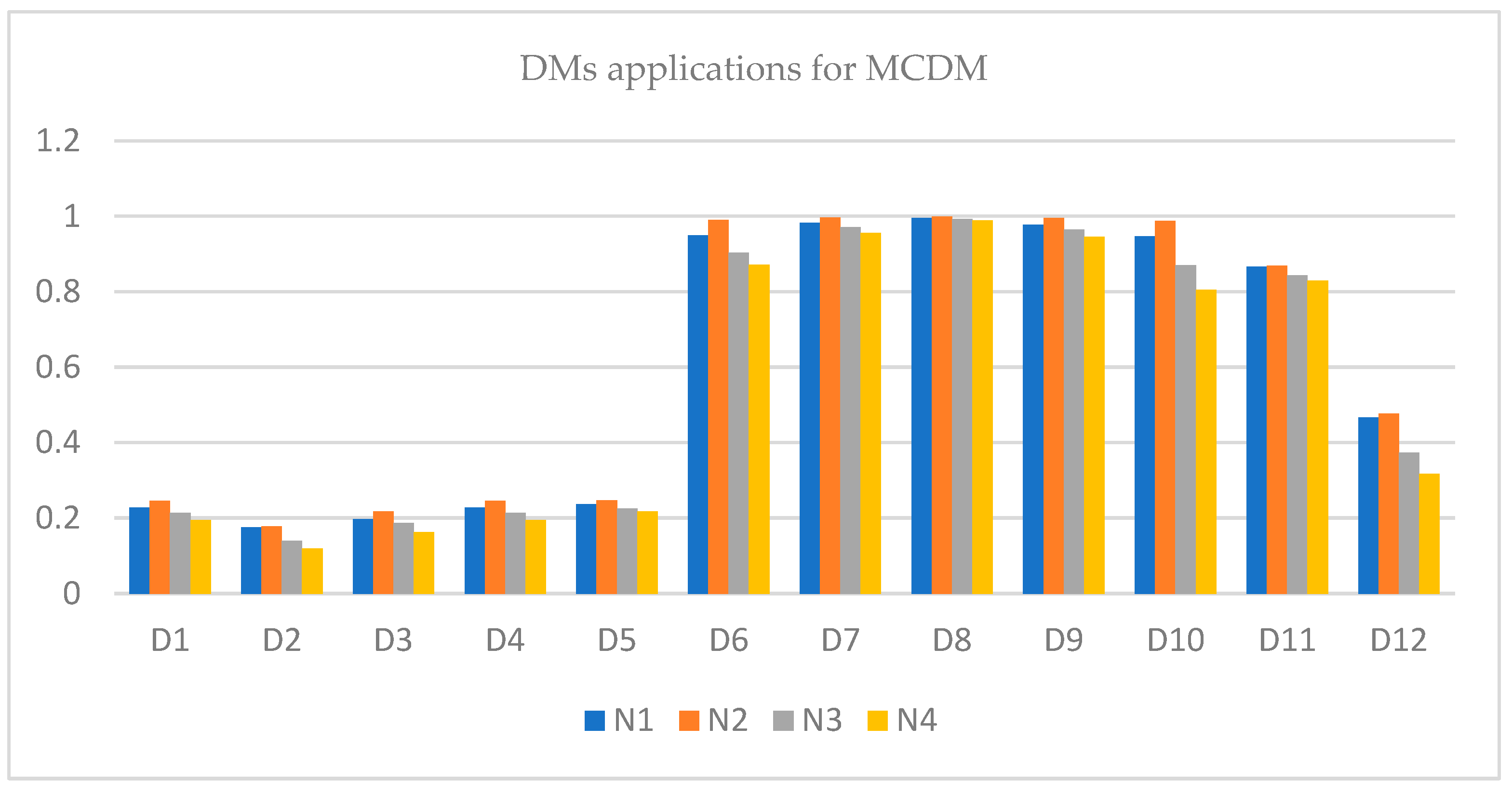
The SM of each TSFN given in
Table 10 is calculated with
, which describes an ideal TSFN, using newly introduced SMs, as shown in
Section 4.
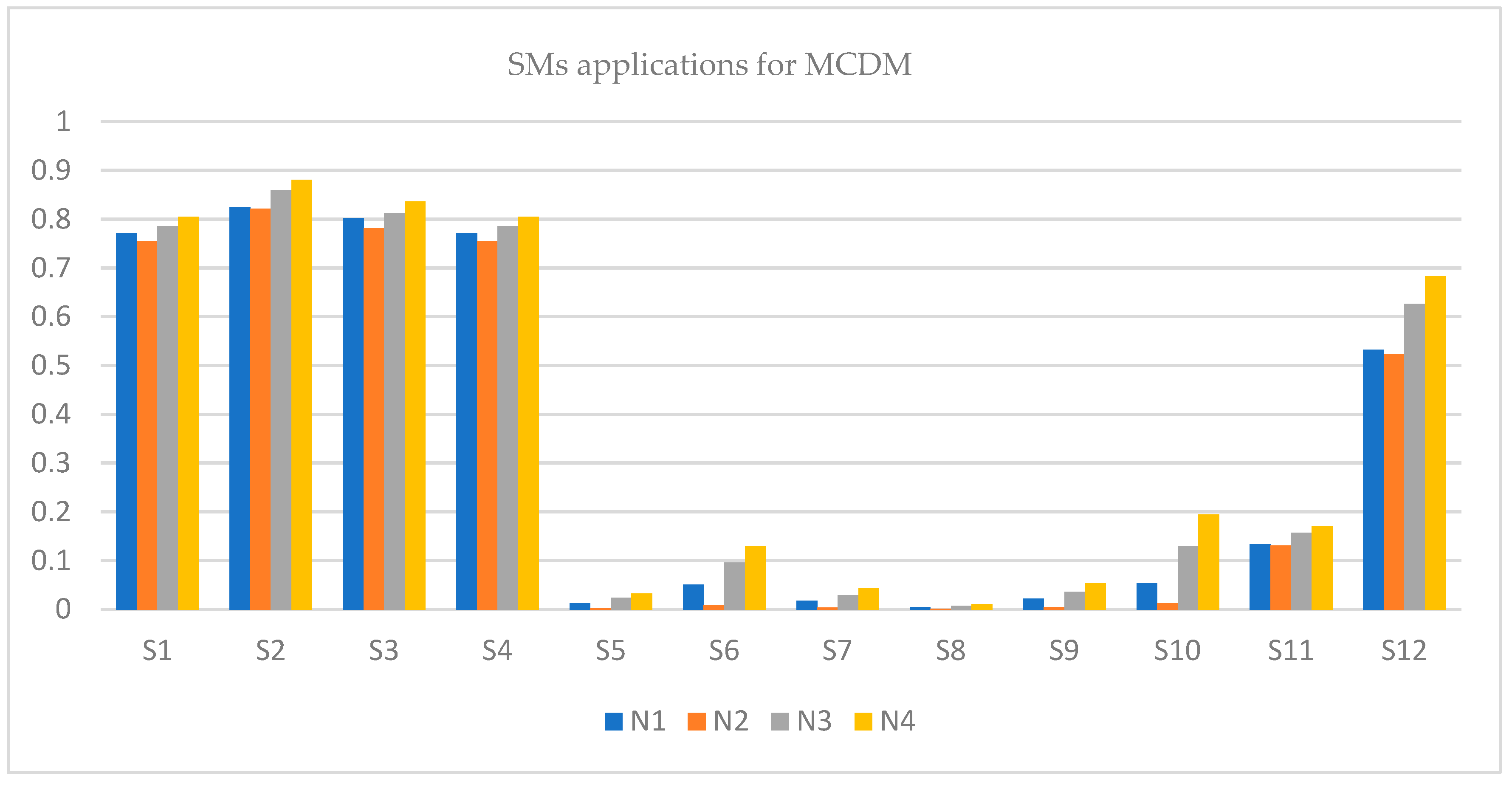
Analyzing
Table 13, for SMs the result obtained is
Hence, is the best choice as the SM of is greater than all the remaining pairs. Furthermore, due to the complex nature of TSFNs, the SMs of IFSs and PFSs cannot be applied to this sort of data.
The outcomes of
Table 13 are portrayed in
Figure 9, which shows that after applying the proposed SMs,
is the best choice for MCDM purposes.
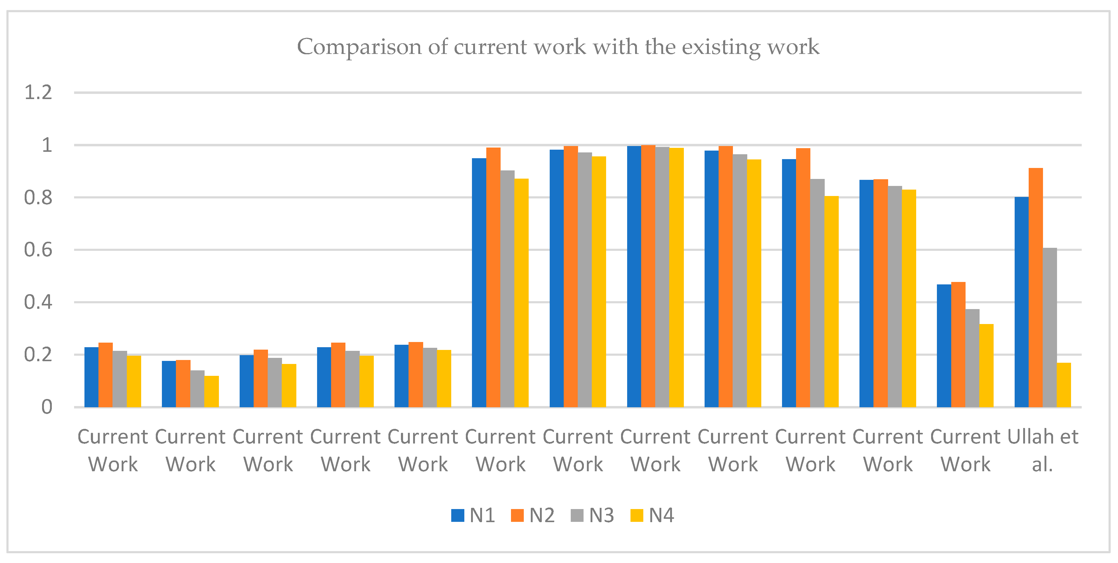
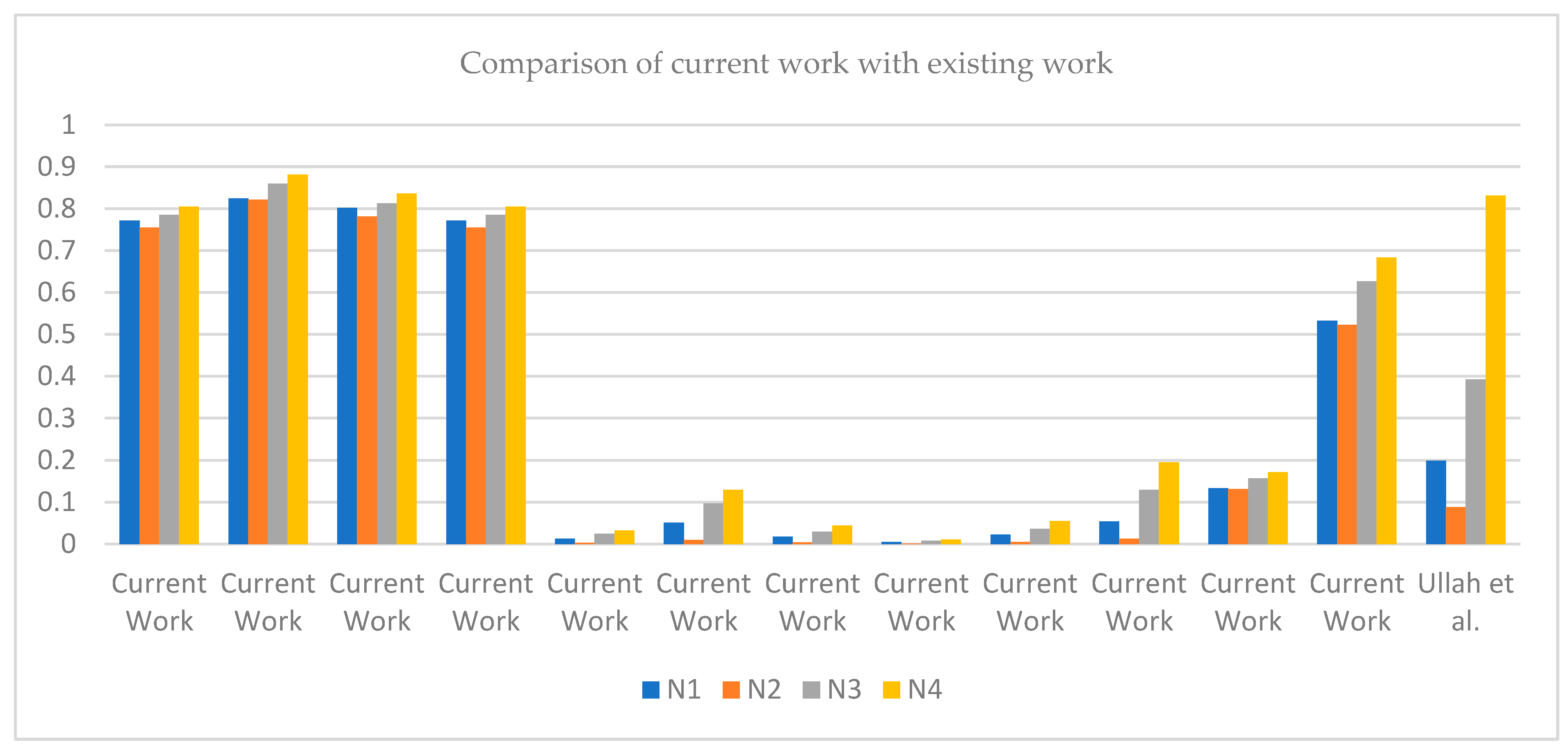
Comparative Study: This section aims to compare the results achieved using SM for TSFSs in the current work with results obtained using SM for TSFSs, as proposed by Ullah et al. [
28]. Here, we also present the limitations of the previously defined SMs of IFSs and PFSs. A brief discussion of the calculated results of this paper compared with other papers is given in
Table 14 below.
The results in
Table 14 support our hypothesis that the SM of TSFSs can manage large amounts of data. The benefit of the introduced SMs is that there are no restrictions on giving values to membership degrees in the environment of TSFSs as it includes all four degrees but there are restrictions on giving values to membership degrees in IFSs, PyFSs, and PFSs. All existing SMs failed to solve the issues due to the absence of RD and restricted range, especially when the data are given in the environment of TSFSs. It is also concluded from
Table 14 that
is the best choice as the SM of
is greater than all the remaining pairs. Therefore, it is said that
is the best choice, which supports our claim.
Figure 10 depicts a comparison of our study with others, and it also explains that our results are suitable and more accurate than those of previous work.


