
On the Chromatic Index of the Signed Generalized Petersen Graph GP(n,2)


1
School of Mathematical Science, Yangzhou University, Yangzhou 225002, China
2
Department of Mathematics, School of Mathematics and Statistics, Guizhou University, Guiyang 550025, China
3
Department of Mathematics, Shanghai University, Shanghai 200444, China
*
Author to whom correspondence should be addressed.
Axioms 2022, 11(8), 393; https://0-doi-org.brum.beds.ac.uk/10.3390/axioms11080393
Submission received: 22 June 2022
/
Revised: 5 August 2022
/
Accepted: 7 August 2022
/
Published: 10 August 2022
(This article belongs to the Special Issue Graph Theory with Applications)
Abstract
:Let G be a graph and be a mapping. The pair , denoted by , is called a signed graph. A (proper) l-edge coloring of is a mapping from each vertex–edge incidence of to such that for each edge , and no two vertex–edge incidences have the same color; that is, . The chromatic index is the minimal number q such that has a proper q-edge coloring, denoted by . In 2020, Behr proved that the chromatic index of a signed graph is its maximum degree or maximum plus one. In this paper, we considered the chromatic index of the signed generalized Petersen graph and show that its chromatic index is its maximum degree for most cases. In detail, we proved that (1) if mod 6; (2) if .
1. Introduction
The graphs considered in this paper are finite and simple. The Petersen graph is a cubic graph with 10 vertices and 15 edges. The Petersen graph appears as a counterexample in many aspects of graph theory. It does not have a 3-edge-coloring proved by Naserasr et al. [1]. The Petersen graph has been widely studied in many aspects of graph theory. Bezrukov et al. [2] defined the nth Cartesian power of Petersen graph and got its cutwidth and wirelength. Then, they generalized these results to the Cartesian product of and m-dimensional binary hypercube. In 1969, Watkins gave the definition of generalized Petersen graph. Let n and k be positive integers with ; then the generalized Petersen graph has vertex set and three types of edges: (i) spoke edges: ; (ii) outer-cycle edges: ; (iii) inner-cycle edges: . All subscripts are modulo n. Obviously, the generalized Petersen graph is a 3-regular graph. The outer-cycle edges form the outer cycle, denoted , and the inner-cycle edges form the inner cycles, denoted , where and . The spoke edges form a perfect matching, denoted . For the edge , the pairs are called the incidences. For terminology and notations not defined here, we refer to [3,4].
Given a graph G and a mapping , the pair , denoted by , is called a signed graph. Here, is a signature of and is the sign of edge e. An edge e is positive if , and it is negative otherwise. We denote by the set of negative edges of . We call graph G the underlying graph of the signed graph . The sign of is the product of the signs of its edges. A cycle is balanced if its sign is and unbalanced otherwise. Switching at a vertex v means negating the sign of every edge that has v as an endpoint. Switching at a vertex set X means switching each in turn. If can be obtained from by switching at some vertices, then we say that they are switching equivalent, denoted by . We also call and equivalent signatures of .
The coloring of signed graphs was first considered by Cartwright and Harry [5]. The coloring of is a mapping from to a color set such that every two vertices joined by a positive edge receive the same color and every two vertices joined by a negative edge receive different colors. They observed that has a 2-coloring if and only if is balanced. In 2016, Máčajová et al. [6] introduced the chromatic number of a signed graph and proved the Brooks’ theorem for signed graph. The proper edge coloring of signed graphs was introduced by Behr [7], and independently, by Zhang et al. [8]. These two definitions are equivalent. Here, we use Behr’s definition, which is based on the signed color set ; that is, if , and = if . A (proper) q-edge coloring of is a mapping from each vertex–edge incidence of to such that for each edge , and no two vertex–edge incidences have the same color; that is, . The chromatic index is the minimal number q such that has a proper n-edge coloring, denoted by . For an edge , if e is negative, and must be colored by the same color, say, c; we can also say that e is colored by c in this case. If e is positive, and must be colored by opposite colors, say, c and ; we also say that e is colored by . Note that every edge can be colored by 0 if .
Zhang et al. [8] mainly showed that if or if G is a planar graph. Behr [7] proved the signed version of Vizing’s theorem; that is, for any signed graph , . The signed graph is type I (type II, respectively) if (, respectively). It is an interesting topic to determine whether a signed graph is type I or type II. The generalized Petersen graph is a famous and well-studied family of graphs. Steimle et al. [9] showed that if n is fixed, when and are isomorphic, there are several properties for the pair . Ralucca et al. [10] studied the spectrum of and added into the family of graphs with known spectra. Ebrahimi et al. [11] proved the necessary and sufficient condition for to have an efficient dominating set, and for several specific cases, authors gave the domination number of . We would like to lay more attention on the coloring of . A Tait coloring of a cubic graph is an edge-coloring in three colors such that each color is incident to each vertex. Castagna et al. [12] proved that all but the original Petersen graph have a Tait coloring. Watkins [13] gave another method to prove that generalized Petersen graphs, except the Petersen graph, have Tait coloring. Khennoufa et al. [14] studied the chromatic number of the edge coloring the total k-labeling of generalized Petersen graphs, and proved that for and , the edge coloring total k-labeling chromatic number of is 3 if n is odd or k is even, and the corresponding chromatic number is 2 if n is even and k is odd. Chen et al. [15] showed that if and , the strong chromatic index of each generalized Petersen graph is at most nine. Li et al. [16] studied the injective edge coloring numbers of and . They got specific values for with , and for with . Yang et al. [17] studied the strong chromatic index of when . In [18], Cai et al. studied the edge coloring of the generalized Petersen graph and got the following results. When , the chromatic index of is three. When , for all signatures but some special cases, the chromatic index of is three. In this paper, we mainly considered the edge coloring of signed generalized Petersen graph , where , and n satisfies certain conditions: (1) mod 6; (2) (). The main aim in this paper is to show that deleting perfect matching of the signed generalized Petersen graph consists of balanced cycles. Note that the perfect matching can be colored by zero, and the left balanced cycles can be colored by ; then, we get a 3-coloring of the signed generalized Petersen graph.
2. Preliminaries
In this section, we introduce some existing properties and results, which can be used to prove our main theorems.
Firstly, we give some notation which will be used in the following paper. Obviously, the generalized Petersen graph has an outer-cycle, , inner-cycles and spokes. For convenience, we use (, respectively) to denote the set of negative edges on the outer cycle (inner cycles, respectively) of . We let . We denote negative edges in spokes set of by . We set . In the same way, , . Let X be a subset of . We used to denote a graph obtained from G by deleting the subset X.
In [7], Behr gave several properties of edge coloring of some special structures of signed graphs.
Lemma 1
([7]). Every signed path can be properly edge colored with (where ). Furthermore, every signed path has exactly two different colorings.
Lemma 2
([7]). A signed cycle C can be properly edge colored with (where ) if and only if C is balanced. Furthermore, every balanced cycle has exactly two different colorings.
Behr also showed that switching does not affect the edge chromatic number of signed graphs.
Lemma 3
([7]). Suppose γ is a proper n-coloring of and is obtained from by switching a vertex set X. Define a new coloring which is obtained from γ by negating all colors on all incidences involving vertices from X. Then, is a proper n-coloring of .
Zaslavsky [19] gave the necessary and sufficient conditions of switching equivalence of two signed graphs and .
Lemma 4
([19]). Two signed graphs and are switching equivalent if and only if they have the same set of unbalanced cycles.
Since we will use matchings of the generalized Petersen graph to complete our proofs, we describe the structures of matchings of generalized Petersen graphs.
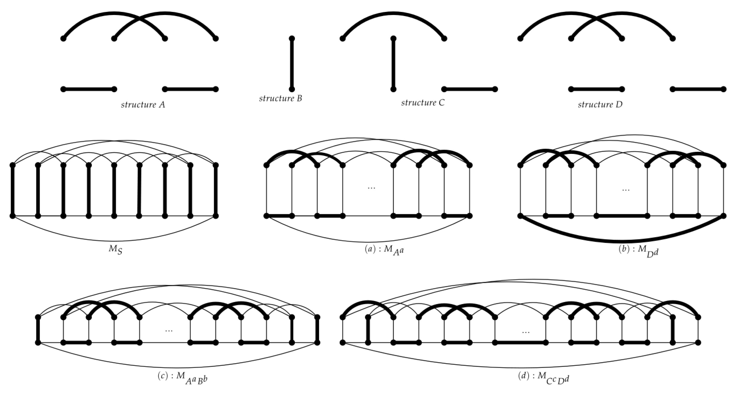
Proposition 1
([20]). Let be the set of perfect matchings of .
(1) For , if there are no spokes in M, then M should be one of the two perfect matchings illustrated in Figure 1(a,b); if there are spokes in M, then the number of spokes between any two consecutive spokes in M is even. Specifically, if there is only one spoke, it implies that n is odd.
(2) Let α denote the number of spokes between any two consecutive spokes in perfect matching M. can be divided into two subsets:
Refer to Proposition 1. We use with to denote perfect matching , and use with to denote .
Cai et al. gave the following lemma and proposition, which also play an important role in our proofs.
Lemma 5
([18]). If has a perfect matching, denoted by , and is formed of balanced cycles, then is 3-edge-colorable.
Proposition 2
([18]). For with any signature σ, let such that is minimized; then all of the following results hold.
(1) , where ;
(2) ;
(3) forms a matching of .
By [20], has the four types of perfect matchings: (1) the matching consists of all spokes, denoted by ; (2) the matching is only formed of structure A(, respectively), denoted by , where ; (3) the matching consists of structures A and B, denoted by , where (here we let these structures A be consecutive; that is, ); (4) the matching consists of structures C and D, denoted by , where (here we let these structures C be consecutive). If n takes some certain values, we can obtain several special perfect matchings of . For proving later results, we make use of the following matchings.
Proposition 3.
There are several perfect matchings of to be used in our proof, which are
(1) and , when mod 6;
(2) , , and , when ;
(3) , and , when .
By Proposition 3, it is easy to check that for mod 6, has the perfect matching . Moreover, the edge set of has special properties. Thus, we give the specific edge set of the perfect matching .
Definition 1.
For mod 6, let and (mod 3),. Furthermore, is a partition of that is and , where .
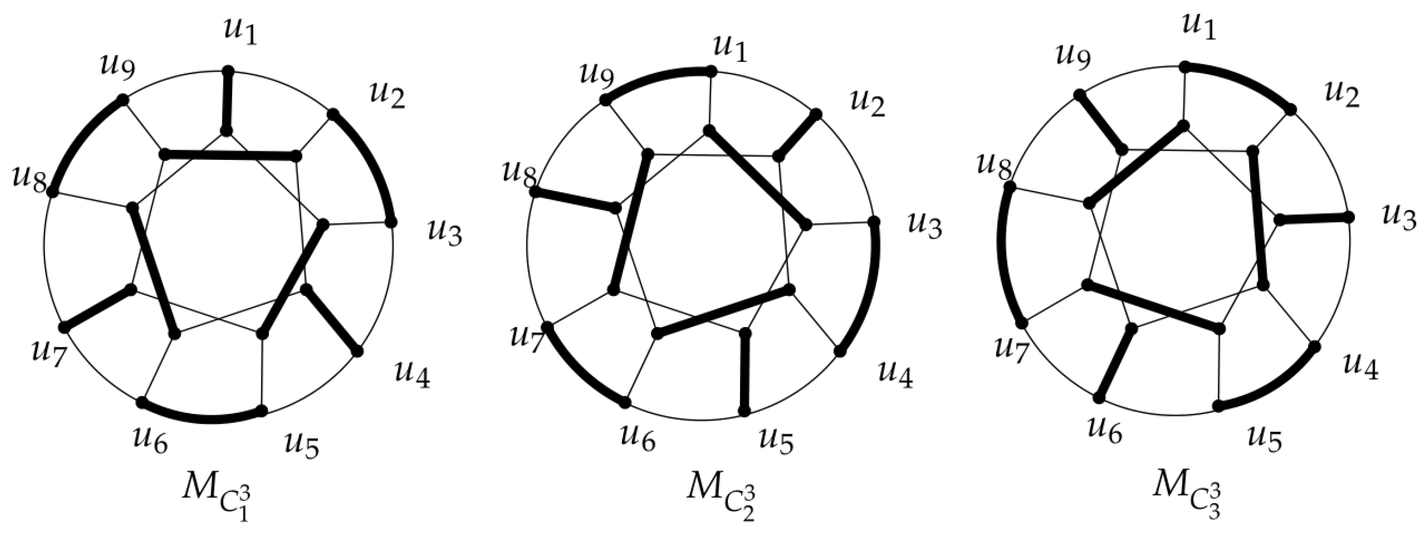
In Figure 2, we give an example of the matching for .
Proposition 4.
If mod 6, is a Hamilton cycle for .
Proof.
Due to symmetry, we prove the case , and other cases can be proved using the same method. All subscripts are modulo n. Let . Firstly, it is easy to check that H is a 2-regular graph. Moreover, H has three kinds of edge: (a) spokes: (mod ; (b) outer-cycle edges: (mod ; (c) inner-cycle edges: (mod .
To show is a Hamilton cycle, we use to denote p 6-paths. It is easy to check that and . Then p 6-paths contain all edges of H. Therefore, H is a Hamilton cycle, that is , where . □
According to Proposition 3, for , there are several special perfect matchings of the generalized Petersen graph . Next, we discuss the graph obtained from by deleting the above perfect matching. If , the generalized Petersen graph has an outer cycle and two inner cycles denoted by and . For convenience, we set . In the following, we characterize several matchings that play an important role in our proofs.
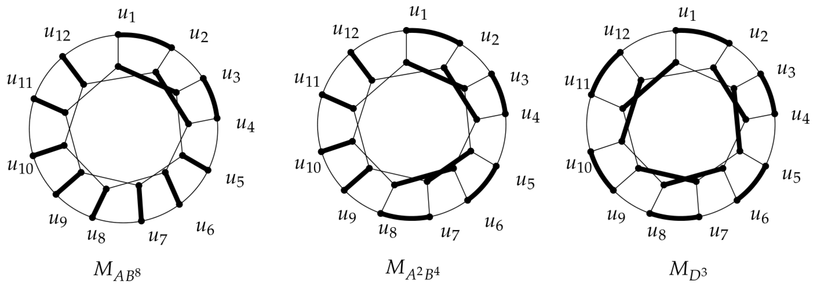
In Figure 3, we depict three kinds of perfect matching of .
Definition 2.
Here we define the edge sets of three special perfect matchings.
Case 1.If , for , the perfect matching has the following edges:
(i) ;
(ii) (mod 4),};
(iii) (mod 4),}.
Case 2.If , for , the perfect matching has the following edges:
(i) ;
(ii) ;
(iii) .
Case 3.If , for , the perfect matching has the following edges:
(i) ;
(ii) ;
(iii) .
Proposition 5.
For and , consists of p cycles.
Proof.
Without loss of generality, we prove the case . Let . It is easy to check that R is a 2-regular graph. Moreover, by Definition 2(case 1), R has three kinds of edge: (a) spokes: all; (b) outer-cycle edges: (mod 4),}; (c) inner-cycle edges: (mod 4),}.
R has p 8-cycles: . Each cycle contains two outer-cycle edges and two inner-cycle edges, and it is easy to check that and . Then, p 8-cycles contain all edges of R. Thus, consists of p 8-cycles, where . □
Proposition 6.
For and , is a Hamilton cycle, where .
Proof.
Let . Without loss of generality, we prove the case . It is easy to check that is a 2-regular graph. All subscripts are modulo n.
(1) When , by Definition 2(case 2), has three kinds of edge: (a) spokes: ; (b) outer-cycle edges: ; (c) inner-cycle edges: .
Firstly, starting at , it passes through ; then it passes the edge to the inner cycle. In the inner cycle it consecutively passes vertices . Here it goes through p inner-cycle vertices with odd subscripts.
Next, it passes the edge to the outer cycle. It will pass vertices . Then, it passes through outer-cycle vertices.
Then, it can pass the edge to the inner cycle. On the inner cycle it will pass . Here it passes through p inner-cycle vertices with even subscripts. Finally, it will pass the edge to the outer cycle. Now we obtain a cycle. Moreover, the cycle passes through all outer-cycle vertices and inner-cycle vertices. Thus, is a Hamilton cycle; that is, .
(2) When , by Definition 2(case 2), has three kinds of edge: (a) spokes: ; (b) outer-cycle edges: ; (c) inner-cycle edges: .
Firstly, starting at , it goes through the following vertices: . Now it passes outer-cycle vertices and inner-cycle vertices with odd subscripts and even subscripts, respectively.
Secondly, it passes the edge to the inner cycle. On the inner cycle it will passes vertices . Here, it passes through inner-cycle vertices with odd subscripts.
Thirdly, it passes the edge to the outer cycle; it passes vertices: . Here it goes through outer-cycle vertices.
Next, it can pass the edge to the inner cycle. In the inner cycle it will passes the following vertices: . Here it passes through inner-cycle vertices with even subscripts.
Finally, it will pass the edge to the outer cycle. Now, we obtain a cycle. Furthermore, the cycle passes through all inner-cycle vertices and outer-cycle vertices. Thus, is Hamilton cycle; that is, . □
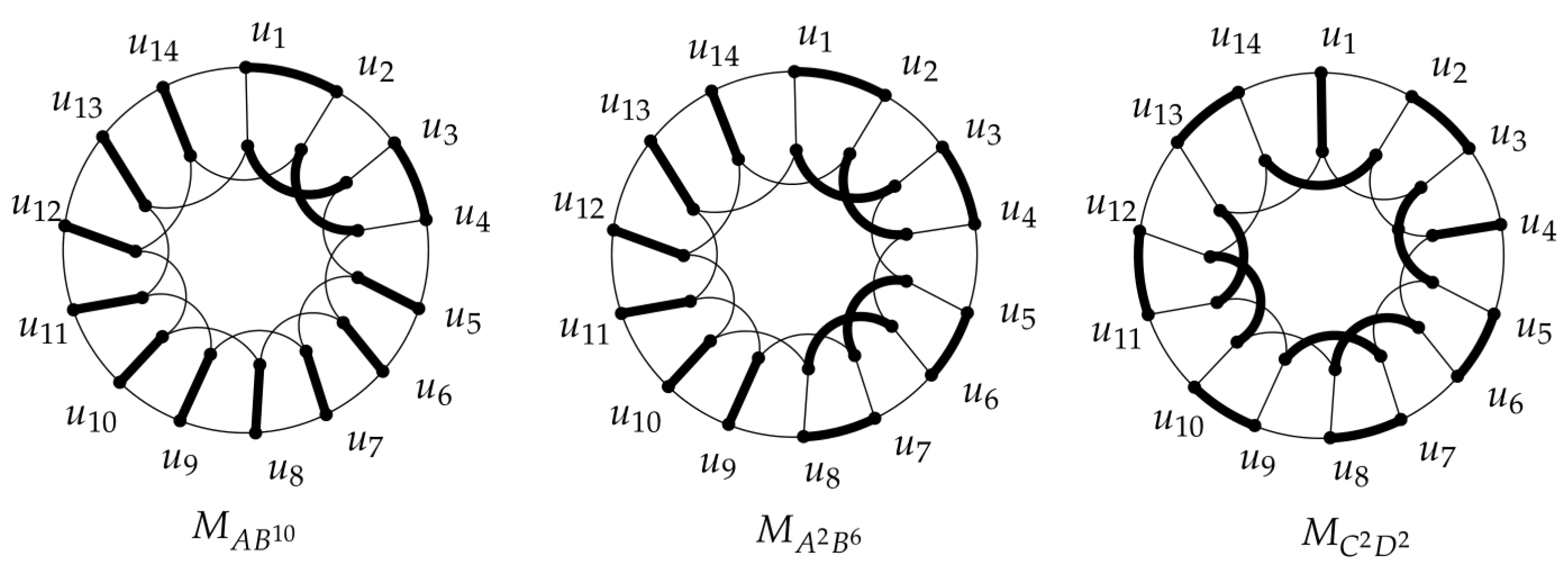
We portray three kinds of perfect matchings of in Figure 4.
Proposition 7.
For and ,
(1) when , is a Hamilton cycle;
(2) when , consists of cycles of length 8 and a cycle of length 20.
Proof.
In the following, we prove the case . Due to symmetry, the other cases can be proved by the same method.
(1) Let . By Definition 2(case 3), then V has three kinds of edge: (a) spokes: ; (b) outer-cycle edges: ; (c) inner-cycle edges: .
Starting at , we can obtain a Hamilton cycle, which is . Thus, V is a Hamilton cycle.
(2) Let . By Definition 2(case 3), has three kinds of edge: (a) spokes: ; (b) outer-cycle edges: ; (c) inner-cycle edges: . The graph consists of outer-cycle edges and inner-cycle edges, respectively, and spokes.
Firstly, starting at point , we obtain a 20-cycle T: . The cycle T consists of six outer-cycle edges, six inner-cycle edges and eight spokes.
Furthermore, starting at points , we get cycles . It is easy to check that , and . Moreover, the 20-cycle and 8-cycles contain all edges of . Thus, consists of 8-cycles and a 20-cycle, where . □
Definition 3.
By Proposition 5, there is always an 8-cycle between two adjacent structures D. Let , and we denote the 8-cycles by . Moreover, , . It is easy to get that .
3. Main Results and Proof
In the following, we introduce our main results and proofs.
For mod 6, the signed generalized Petersen graph has perfect matchings . Next, we study the parity of and .
Lemma 6.
For any signature σ, mod 6. Let and . If and have opposite parity, then and have opposite parity.
Proof.
Without loss of generality, we assume that is odd and is even. By the Definition 1, is odd. Then, and have opposite parity, since . □
By Proposition 2, each cycle has at most one negative edge. If , due to symmetry, we can assume that the negative edge is on the outer cycle.
Lemma 7.
Let . For , if and have opposite parity, then is a balanced Hamilton cycle.
Proof.
According to Proposition 4, we know that is a Hamilton cycle. Without loss of generality, for , if we assume that is odd and is even, then is odd. For , it is easy to check that . There are even negative edges in the Hamilton cycle. Thus, is a balanced Hamilton cycle. □
In the following, we consider the case that there is a negative edge on each cycle.
Lemma 8.
Let . For , if and have the same parity, then is a balanced Hamilton cycle.
Proof.
. It is easy to check that and have the same parity. If and have the same parity, then and have the same parity. Therefore, is a balanced Hamilton cycle. □
The following theorem settles the issue for , mod 6.
Theorem 1.
For any σ, , where mod 6.
Proof.
Firstly, we show that there is always a perfect matching M such that consists of balanced cycles.
Claim 1.
For mod 6, there must be a perfect matching M such that consists of balanced cycles.
Proof of Claim 1.
When mod 6, the generalized Petersen graph has an outer cycle and an inner cycle since . Let such that is minimized. According to Proposition 2, , . In the following, we continue the proof according to the number of negative edges on the outer cycle and the inner cycle.
Case 1. and .
In this case, ; then, consists of two balanced cycles.
If , then the negative edge may be on the outer cycle or the inner cycle. Due to symmetry, we assume that the negative edge is on the outer cycle. By Proposition 4, is a Hamilton cycle.
Case 2. and .
Without loss of generality, let . In this case, for , . If and have the same parity, then is even. Thus, is a balanced Hamilton cycle, since . If and have opposite parity, then by Lemma 6, and have opposite parity. There must be a matching such that and have opposite parity for . By Lemma 7, is a balanced Hamilton cycle.
Case 3. and .
Let . We continue our proof according to whether the edge is on the matching .
Subcase 3.1..
In this case, is even for . It is not difficult to get that . If and have the same parity, then and have the same parity. By Lemma 8, is a balanced Hamilton cycle. If and have opposite parity, then by Lemma 6, and have opposite parity. There must be a matching such that and have the same parity for , so and have the same parity. By Lemma 8, is a balanced Hamilton cycle.
Subcase 3.2..
By Definition 1, are a partition of . As , for . Due to symmetry, we only consider the case . In this case, is odd for and is even. It is not difficult to get that . If and have the same parity, then and have the same parity. By Lemma 8, is a balanced Hamilton cycle. If and have opposite parity, then by Lemma 6, and have opposite parity. There must be a matching such that and have opposite parity for , so and have the same parity. By Lemma 8, is a balanced Hamilton cycle. □
By Claim 1, there is always a matching M such that consists of balanced cycles. Then, by Lemma 5, where mod 6. □
In the following, we study the edge coloring of the generalized Petersen graph for any signature and .
Lemma 9.
Let . For , if we can find a matching satisfying one of the following conditions:
(i) is odd. and have opposite parity.
(ii) is even. and have the same parity.
Then is a balanced Hamilton cycle.
Proof.
By Proposition 6, is a Hamilton cycle.
(i) It is easy to check that . When is odd, and have opposite parity. Since and have opposite parity, and have the same parity. Moreover, , so contains even negative edges. Therefore, is a balanced Hamilton cycle.
(ii) It is easy to check that . When is even, and have the same parity. Since and have the same parity, and have the same parity. Moreover, , so contains even negative edges. Therefore, is a balanced Hamilton cycle. □
Theorem 2.
For any σ, , where .
Proof.
Firstly, we show that there is always a perfect matching M such that consists of balanced cycles.
Claim 2.
For , there must be a perfect matching M such that consists of balanced cycles.
Proof of Claim 2.
If , then the generalized Petersen graph has an outer cycle and two inner cycles . Let such that is minimized. According to Proposition 2, each cycle has at most one negative edge. In the following, we continue the proof according to the number of negative edges on cycles.
Case 1. is odd.
In the following, we continue our discussion according to the parity of p.
Subcase 1.1.p is an odd integer.
Let . It is easy to check that is a Hamilton cycle for . By Lemma 9(i), if we can find a matching satisfying the condition, then is a balanced Hamilton cycle. Otherwise, for arbitrary i, and have the same parity.
If , by Proposition 7, is a Hamilton cycle. We denote the Hamilton cycle by T. We set , where . It is easy to check that for by Definition 3. Since and have the same parity, is even. Furthermore, , so is even. Therefore, T is a balanced Hamilton cycle.
If , by Proposition 7, consists of a 20-cycle and 8-cycles. Firstly, we denote the 20-cycle by T. Let , where . By Definition 3, it is easy to check that for , where . Since and have the same parity, is even. Furthermore, , so is even. Therefore, T is a balanced cycle. Next, by Definition 3, we denote 8-cycles by . Then, , where . Since , . Since and have the same parity, is even. Therefore, 8-cycles are balanced.
Subcase 1.2.p is an even integer.
In this case, we continue our proof by using the matching . By Proposition 5, consists of p 8-cycles. By Definition 3, we denote the p 8-cycles by (mod 4)}. Then, , where . Since , . Since and have the same parity, every 8-cycle contains even negative edges. Therefore, consists of p balanced cycles.
Case 2. is even.
By Lemma 9(ii), if we can find a matching satisfying the condition, then is a balanced Hamilton cycle. Otherwise, for arbitrary i, and have opposite parity.
Next, we continue our proof by using the matching . Let . By Proposition 6, it is easy to know that is a Hamilton cycle. For arbitrary i, , . If and have the same parity, then and have the same parity. If and have opposite parity, then and have opposite parity. Thus, and have the same parity. By Lemma 9, is a balanced Hamilton cycle. □
According to Claim 2, for , there is always a perfect matching M such that consists of balanced cycles. Thus, according to Lemma 5, for . □
4. Conclusions
In this paper, we proved that (1) if mod 6; (2) if , . For , there are still two unsolved cases, which are mod 6 and mod 6. When mod 6, is not a Hamilton cycle, and when mod 6, itself is not Hamiltonian. Thus, our method in this paper is not suitable for these two cases, which is one subject of our future work. In addition, it is also an interesting and challenging problem to consider for , since there is no characterization of perfect matchings of .
Author Contributions
Supervision, Q.S.; Writing—original draft, S.Z. and Q.S.; Writing—review & editing, H.C., Y.W. and Q.S. All authors have read and agreed to the published version of the manuscript.
Funding
This research was funded by National Natural Science Foundation of China (Nos.11801494, 11971196).
Institutional Review Board Statement
Not applicable.
Informed Consent Statement
Not applicable.
Acknowledgments
The authors would like to thank referees for their helpful comments.
Conflicts of Interest
The authors declare no conflict of interest.
References
- Naserasr, R.; Škrekovski, R. The Petersen graph is not 3-edge-colorable—A new proof. Discret. Math. 2003, 268, 325–326. [Google Scholar] [CrossRef]
- Bezrukov, S.; Das, S.; Elsässer, R. An Edge-Isoperimetric Problem for Powers of the Petersen Graph. Ann. Comb. 2000, 4, 153–169. [Google Scholar] [CrossRef]
- Murty, U.S.R.; Bondy, A. Graph Theory; Graduate Texts in Mathematics; Springer: London, UK, 2008; Volume 244. [Google Scholar]
- Diestel, R. Graph Theory, 4th ed.; Graduate Texts in Mathematics; Springer: Berlin/Heidelberg, Germany, 2008. [Google Scholar]
- Cartwright, D.; Harary, F. On the coloring of signed graphs. Elem. Math. 1968, 23, 85–89. [Google Scholar]
- Máčajová, E.; Raspaud, A.; škoviera, M. The chromatic number of a signed graph. Electron. J. Comb. 2016, 23, 1–14. [Google Scholar] [CrossRef]
- Behr, R. Edge coloring signed graphs. Discret. Math. 2020, 343, 111654. [Google Scholar] [CrossRef]
- Zhang, L.; Lu, Y.; Luo, R.; Ye, D.; Zhang, S. Edge coloring of signed graphs. Discret. Appl. Math. 2020, 282, 234–242. [Google Scholar] [CrossRef]
- Steimle, A.; Staton, W. The isomorphism classes of the generalized Petersen graphs. Discret. Math. 2009, 309, 231–237. [Google Scholar] [CrossRef]
- Ralucca, G.; Stănică, P. The spectrum of generalized Petersen graphs. Australas. J. Comb. 2011, 49, 39–46. [Google Scholar]
- Ebrahimi, B.; Jahanbakht, N.; Mahmoodian, E. Vertex domination of generalized Petersen graphs. Discret. Math. 2009, 309, 4355–4361. [Google Scholar] [CrossRef]
- Castagna, F.; Prins, G. Every generalized Petersen graph has a Tait coloring. Pac. J. Math. 1972, 40, 53–58. [Google Scholar] [CrossRef]
- Watkins, E. A theorem on Tait colorings with an application to the generalized Petersen graphs. J. Comb. Theory 1969, 6, 152–164. [Google Scholar] [CrossRef]
- Khennoufa, R.; Seba, H. Edge coloring total k-labeling of generalized Petersen graphs. Inf. Process. Lett. 2013, 113, 489–494. [Google Scholar] [CrossRef]
- Chen, M.; Miao, L.; Zhou, S. Strong Edge Coloring of Generalized Petersen Graphs. Mathematics 2020, 8, 1265. [Google Scholar] [CrossRef]
- Li, Y.; Chen, L. Injective edge coloring of generalized Petersen graphs. AIMS Math. 2021, 6, 7279–7943. [Google Scholar] [CrossRef]
- Yang, Z.; Wu, B. Strong edge chromatic index of the generalized Petersen graphs. Appl. Math. Comput. 2008, 321, 431–441. [Google Scholar] [CrossRef]
- Cai, H.; Sun, Q.; Xu, G.; Zheng, S. Edge Coloring of the signed generalized Petersen Graph. Bull. Malays. Math. Sci. Soc. 2022, 45, 647–661. [Google Scholar] [CrossRef]
- Zaslavsky, T. Signed graphs. Discret. Appl. Math. 1982, 4, 47–74. [Google Scholar] [CrossRef]
- Zhao, S.; Zhu, J.; Zhang, H. On the forcing spectrum of generalized Petersen graph P(n, 2). arXiv 2017, arXiv:1707.03701. [Google Scholar]
Figure 1.
All types of perfect matchings of . Here, bold lines denote the edges in the perfect matching.
Figure 1.
All types of perfect matchings of . Here, bold lines denote the edges in the perfect matching.

Figure 2.
The matching of . Here bold lines denote the edges in the perfect matching.

Figure 3.
For , the perfect matchings and of . Here, bold lines denote the edges in the perfect matching.
Figure 3.
For , the perfect matchings and of . Here, bold lines denote the edges in the perfect matching.

Figure 4.
For , the perfect matchings and of . Here, bold lines denote the edges in the perfect matching.
Figure 4.
For , the perfect matchings and of . Here, bold lines denote the edges in the perfect matching.

Publisher’s Note: MDPI stays neutral with regard to jurisdictional claims in published maps and institutional affiliations. |
© 2022 by the authors. Licensee MDPI, Basel, Switzerland. This article is an open access article distributed under the terms and conditions of the Creative Commons Attribution (CC BY) license (https://creativecommons.org/licenses/by/4.0/).
Share and Cite
MDPI and ACS Style
Zheng, S.; Cai, H.; Wang, Y.; Sun, Q. On the Chromatic Index of the Signed Generalized Petersen Graph GP(n,2). Axioms 2022, 11, 393. https://0-doi-org.brum.beds.ac.uk/10.3390/axioms11080393
AMA Style
Zheng S, Cai H, Wang Y, Sun Q. On the Chromatic Index of the Signed Generalized Petersen Graph GP(n,2). Axioms. 2022; 11(8):393. https://0-doi-org.brum.beds.ac.uk/10.3390/axioms11080393
Chicago/Turabian StyleZheng, Shanshan, Hongyan Cai, Yuanpei Wang, and Qiang Sun. 2022. "On the Chromatic Index of the Signed Generalized Petersen Graph GP(n,2)" Axioms 11, no. 8: 393. https://0-doi-org.brum.beds.ac.uk/10.3390/axioms11080393
Note that from the first issue of 2016, this journal uses article numbers instead of page numbers. See further details here.