Article

Color Image Recovery Using Generalized Matrix Completion over Higher-Order Finite Dimensional Algebra

1
School of Electronics and Information, Zhongyuan University of Technology, Zhengzhou 451191, China
2
Birkbeck College, University of London, London WC1E 7HY, UK
3
School of Information Engineering, Zhengzhou University, Zhengzhou 450001, China
*
Author to whom correspondence should be addressed.
Submission received: 6 August 2023 / Revised: 23 September 2023 / Accepted: 7 October 2023 / Published: 10 October 2023

Abstract

:
To improve the accuracy of color image completion with missing entries, we present a recovery method based on generalized higher-order scalars. We extend the traditional second-order matrix model to a more comprehensive higher-order matrix equivalent, called the “t-matrix” model, which incorporates a pixel neighborhood expansion strategy to characterize the local pixel constraints. This “t-matrix” model is then used to extend some commonly used matrix and tensor completion algorithms to their higher-order versions. We perform extensive experiments on various algorithms using simulated data and publicly available images. The results show that our generalized matrix completion model and the corresponding algorithm compare favorably with their lower-order tensor and conventional matrix counterparts.

1. Introduction

1.1. Background and Related Works

Vectors and matrices are fundamental to data analysis and processing, but it is often a struggle to encapsulate the complex, higher-order structures found in data such as color images, video sequences, and hyperspectral images. These multilinear data structures defy satisfactory representation by traditional vectors and matrices, prompting the use of tensors, i.e., higher-order extensions of vectors and matrices, for more accurate representation.
In real-world scenarios, it is common to find that high dimensional data often have low intrinsic dimensions. This property facilitates several advanced techniques and applications. For example, Floryan et al. [1] reduce data to their intrinsic dimensions, allowing more accurate and low-dimensional dynamical models to capture the essential behavior of high-dimensional systems with low-dimensional features. Li et al. [2] achieve efficiency and robustness by training deep neural networks in low-dimensional spaces without sacrificing performance. Chen et al. [3] use deep learning networks for nonparametric regression on low-dimensional manifolds, emphasizing the adaptability of the networks to low-dimensional geometric structures in data. Xu et al. [4] propose a method that improves high-dimensional data classification through efficient feature extraction and diverse feature fusion, outperforming mainstream ensemble methods.
This notion of a low intrinsic dimension often applies when the data are represented as matrices or tensors. Several methods take advantage of this property. Fu et al. [5] develop a low-rank tensor approximation model for multiview intrinsic subspace clustering that effectively reduces view-specific constraints and improves optimization, with notable success on real-world datasets. Wang et al.’s [6] tensor low-rank and sparse representation method skillfully preserves intrinsic 3D structures in hyperspectral anomaly detection. In addition, Liu et al. [7] comprehensively survey low-rank tensor approximation for hyperspectral image restoration, highlighting state-of-the-art techniques and current challenges in the field. This collective body of work underscores the flexibility and potential of using low-rank approximations to manage and interpret complex, high-dimensional data.
The collection of high-dimensional data can result in the loss of some elements. Low-rank tensor completion (LRTC) addresses this problem by reconstructing the missing components from known data elements. Unlike low-rank matrix completion (LRMC), which relies solely on second-order information, LRTC exploits higher-order information, making the study of low-rank tensor completion techniques an important frontier in many fields.
For example, Liu et al. [8] introduced the Sum of Matricization-based Nuclear Norms (SMNN), which is based on the Tucker rank of the tensor, and formulated three optimization algorithms for tensor completion via SMNN minimization, successfully applying them to visual data completion. Zhang et al. [9,10] developed the tubal nuclear norm (tubal-NN) approach based on the tubal-rank tensor, and designed an algorithm that uses tensor nuclear norm penalization for tensor completion. The algorithm is effective in video recovery and denoising. Lu et al. [11] constructed a tensor completion model using the tensor nuclear norm (TNN). They showed that the TNN is a specific atomic norm, and established a bound for guaranteed low-tubal-rank tensor recovery, thus providing recovery guarantees for tensor completion. Xue et al. [12] extended the tensor completion model to include the tensor truncated nuclear norm (T-TNN), thereby improving its effectiveness in real-world video and image processing.
In addition to these newly defined tensor norms, researchers are now developing other techniques that extend traditional concepts to new applications in tensor completion. For example, Zeng et al. [13] introduced a multimodal nuclear tensor factorization technique, which incorporates low-rank insights and an efficient block successive upper-bound minimization algorithm. The method was applied to tasks such as hyperspectral images, video, and MRI completion, with experimental results confirming its superior performance. Similarly, Wu et al. [14] presented the tensor wheel decomposition method, which characterizes complex interactions with only a few hyperparameters, improving performance on both synthetic and real data. Zhao et al. [15] presented a nonconvex model with a proximal majorization–minimization algorithm for robust low-rank tensor completion, providing theoretical guarantees and demonstrating high efficiency on visual data, including color and multispectral images.
In recommendation systems, Deng et al. [16] applied a meta-learning strategy with low-rank tensor completion for hyperparameter optimization and demonstrated its effectiveness. Nguyen [17] developed a consistency-based framework that emphasizes unit-scale consistency for matrix and tensor completion, with attributes such as fairness and the ability to exploit high-dimensional relationships. Hui et al. [18] integrated social–spatial context into tensor completion for time-aware point-of-interest recommendations, outperforming existing methods.
Tensor completion has also contributed to advance in data mining. Song et al. [19] reviewed recent tensor completion algorithms, examining four perspectives and various applications in data mining. Wu et al. [20] introduced a multiattentional tensor completion network for handling missing entries in road sensor data, demonstrating improved performance. Lee et al.’s [21] sign representable tensor model addresses both low and high rank signals for tensor completion, improving performance on human brain connectivity and topic data mining datasets.

1.2. Contributions and Organization of This Paper

Building on the success of low-rank tensor completion (LRTC) as compared with low-rank matrix completion (LRMC), this paper takes a leap forward by employing a higher-order t-matrix model with high-order circular convolution. This novel method forms a specific generalization of LRMC tailored to multi-way image recovery, including the completion of RGB images with missing entries.
Our model is inspired by the well-regarded completion algorithm proposed by Lu et al. [11]. Our model extends Lu et al.’s algorithm by incorporating a high-order methodology for high-dimensional data. Evaluations of our approach demonstrate competitive recovery performance, with favorable recovery performance compared to existing algorithms.
The practical implications of this work are multifaceted, providing solutions that not only improve visual data completion, but also offer broader applications in areas such as video recovery, data mining, and medical imaging. By integrating our higher-order generalization into existing systems, it is possible to create more efficient and robust mechanisms for handling high-order, high-dimensional data.
The contributions of this research are summarized as follows.
  • This research presents a t-matrix model that can extend traditional matrix methods to a higher order. The higher-order algorithm, termed “Higher-Order TNN”, is designed to exploit intricate structures in high-dimensional data and refines classical lower-order algorithms for missing entry recovery of RGB images. Compared to its predecessors, Higher-Order TNN offers significantly improved recovery performance.
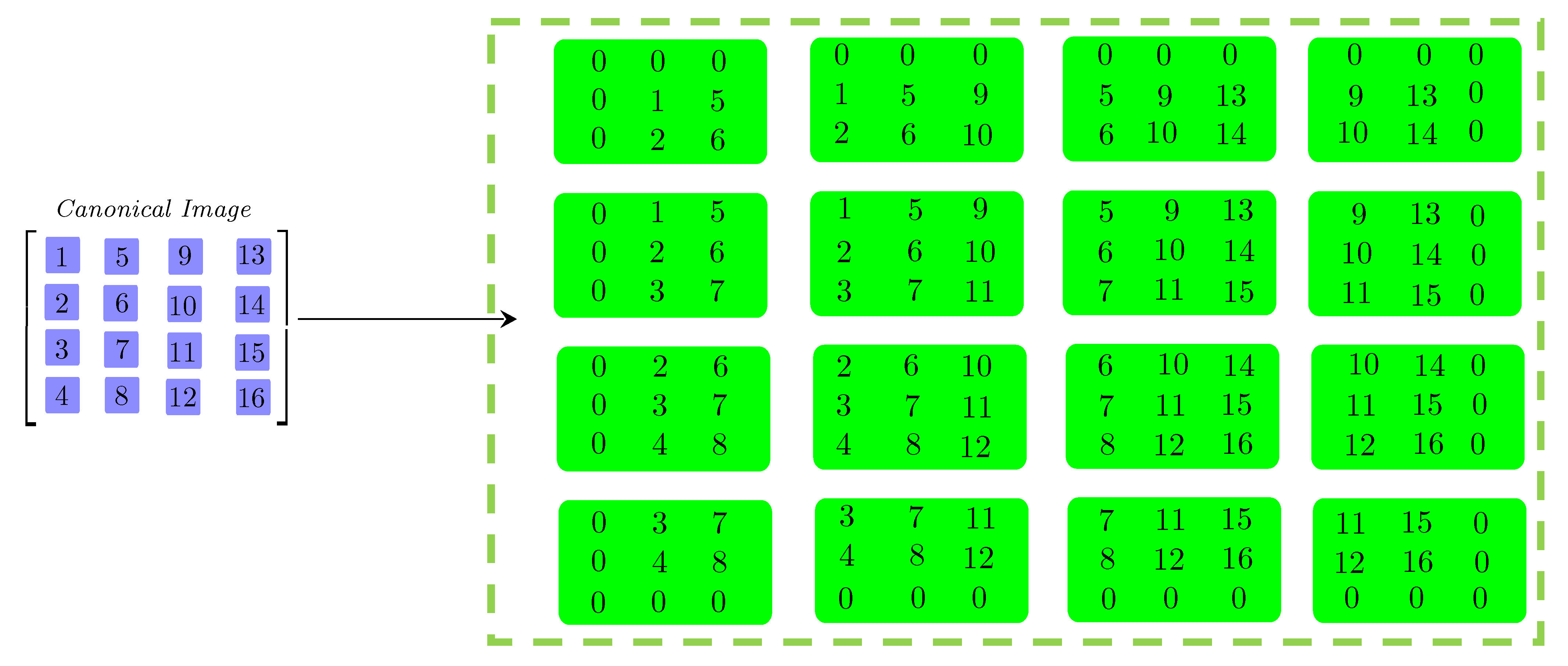
  • Using the t-matrix model over a finite-dimensional algebra, several image analysis algorithms are extended to a higher order using a novel pixel neighborhood strategy.
  • Many constructions in matrix and vector analysis are extended to the t-matrix model. Examples include rank, norm, and inner product. In addition, t-matrix versions of Lagrange multipliers are defined.
The rest of the paper is organized as follows: Section 2 introduces t-matrices, outlining their structure, representation, and possible extension. Section 3 describes the low-rank matrix completion (LRMC) methodology and its higher-order counterparts, explaining the use of t-scalars and t-matrices. Section 4 provides an in-depth exploration of rank considerations, presenting different notions of rank and the concept of higher-order rank. Section 5 details experimental validation and performance analysis, using both simulated random data and real-world datasets such as the Berkeley Segmentation Dataset. Section 6 summarizes the content of this paper and its implications. Appendix A provides further mathematical justification, explaining the mechanism of t-scalars and t-matrices from a unique matrix perspective of representation and operator theory, along with an exploration of the Lagrange multiplier with t-matrix variables.

2. T-Matrices

A t-matrix is a rectangular array composed of elements called t-scalars [22]. Since a t-scalar forms an array in C I 1 × × I N , a t-matrix with D 1 rows and D 2 columns can be represented by a multiway complex array in C I 1 × × I N × D 1 × D 2 . While various authors [23,24], including Kilmer et al. [10], categorize these t-matrices as tensors, we use the term “t-matrix over t-scalars”. The t-matrix model is used to extend many existing matrix algorithms.

2.1. T-Scalars

A complex array of order N is by definition an element of the set C, where C C I 1 × × I N . Similarly, a real array of order N is an element of the set R, where R R I 1 × × I N . The sets R and C share a commutative ring structure, in which the multiplication is defined by a circular convolution of order N and the addition is entry-wise. Elements of C and R are called t-scalars. In this paper, we focus primarily on C, since R is a subset of C. By further defining the multiplication of a t-scalar with a complex number by conventional scalar multiplication, we can elevate the ring C to a finite dimensional commutative algebra.
Using t-scalars not only allows us to construct novel matrices, but also allows the extension of many classical matrix algorithms into the realm of t-matrix algorithms.
We adopt the notions described by Liao and Maybank [22]. For example, the following definitions are given for t-scalars.
Definition 1
(Addition of T-scalars [22]). Consider two t-scalars x ˙ , y ˙ C I 1 × × I N as order-N arrays of size I 1 × × I N . The sum, c ˙ = x ˙ + y ˙ , with c ˙ C I 1 × × I N , is calculated element-wise,
( c ˙ ) i 1 , , i N = ( x ˙ ) i 1 , , i N + ( y ˙ ) i 1 , , i N i 1 , , i N .
Definition 2
(Multiplication of T-scalars [22]). Let x ˙ , y ˙ C I 1 × × I N be two t-scalars of size I 1 × × I N . Their product is defined as c ˙ = x ˙ y ˙ , where c ˙ results from the order-N circular convolution of x ˙ and y ˙ . Specifically, we have
( c ˙ ) i 1 , , i N = ( k 1 , , k N ) [ I 1 ] × × [ I N ] ( x ˙ ) k 1 , , k N · ( y ˙ ) k 1 , , k N , i 1 , , i N
where k n = mod ( i n k n , I n ) + 1 , for all n [ N ] .
Although order-two t-scalars share the data structure of order-two numerical arrays, they differ from matrices in that their multiplication is commutative. Nevertheless, when a linear transformation, such as the Fourier transform, is applied to a t-scalar, it is convenient to think of the underlying order-two arrays of t-scalars as matrices. This principle extends to higher-order t-scalars as well. When a multilinear transformation is applied to a higher-order t-scalar, the underlying higher-order array of the t-scalar can be treated as a tensor.
We use the notation tensor ( x ˙ ) to elevate the underlying order-N array of x ˙ to a conventional tensor of identical size and entries. With tensor ( x ˙ ) as the conventional tensor, the multiplication of two t-scalars is given in the Fourier domain by the following theorem.
Theorem 1
(Fourier Transform). Let x ˙ , y ˙ C be two t-scalars with the product c ˙ = x ˙ y ˙ C . Define x ˜ = F ( x ˙ ) , y ˜ = F ( y ˙ ) , and c ˜ F ( c ˙ ) as their respective multilinear Fourier transforms. For any t-scalar x ˙ C , its multilinear Fourier transform is given by the following multi-mode multiplication:
F ( x ˙ ) tensor ( x ˙ ) × 1 W 1 × n W n × N W N
where W n denotes the I n × I n Fourier matrix such that the following equation holds for all k 1 , k 2 [ I n ] ,
( W n ) k 1 , k 2 = exp 2 π I n 1 1 ( k 1 1 ) ( k 2 1 ) .
Consequently, the following Hadamard product holds for all i 1 , , i N :
( c ˜ ) i 1 , , i N = ( x ˜ ) i 1 , , i N · ( y ˜ ) i 1 , , i N .
Definitions 1 and 2 qualify all t-scalars as elements of a commutative ring C. An essential operation in C is the multiplication of elements of C with a scalar. This leads to the following definition.
Definition 3
(Scalar Multiplication [22]). Let x ˙ C C I 1 × × I N be a t-scalar and λ a complex number. Their multiplication, denoted as y ˙ λ · x ˙ C , is defined for all i 1 , , i N as follows:
( y ˙ ) i 1 , , i N = λ · ( x ˙ ) i 1 , , i N .
With the above definitions as a basis, we have the following proposition about the identity and zero t-scalars in the algebra C.
Proposition 1
(Identity T-scalar and Zero T-scalar [22]). Consider a t-scalar e ˙ C I 1 × × I N . In this case, ( e ˙ ) i 1 , , i N = 1 if i 1 = = i N = 1 , and ( e ˙ ) i 1 , , i N = 0 otherwise. Alternatively, if every entry of x ˙ is 0, we have this t-scalar as the zero t-scalar z ˙ . Note that each entry of the identity t-scalar is 1 in the Fourier domain, while the zero t-scalar remains unchanged in the Fourier domain.

2.2. T-Scalars as Finite-Dimensional Linear Operators

Since every t-scalar in the algebra C defines a commutative finite dimensional linear operator, operator theory allows us to determine the spectrum of any t-scalar x ˙ C . The spectrum, or the set of complex eigenvalues of x ˙ , corresponds to the K entries of the Fourier transform x ˜ (where K I 1 · I 2 I N ), taking multiplicity into account.
The eigenvalues, i.e., Fourier entries, of a t-scalar help to define concepts such as trace, Schatten norm, and singular values of a t-scalar. The following definitions are presented first, before a more detailed exploration of the above concepts later in this paper.
Definition 4
(Conjugate [22]). A unique t-scalar y ˙ in C is the conjugate of a t-scalar x ˙ in C if each eigenvalue of y ˙ is the complex conjugate of the corresponding eigenvalue of x ˙ . The conjugate is denoted by x ˙ * .
Definition 5
(Non-negativity [22]). A t-scalar x ˙ is said to be non-negative if and only if all of its complex eigenvalues (i.e., Fourier entries) are non-negative real numbers.
Definition 5 is crucial because it facilitates the generalization of various concepts of non-negativity, including matrix rank, space dimension, norm, and distance, to non-negative elements in C. We explore these generalizations below, as needed.
Consider any two non-negative t-scalars x ˙ , y ˙ . Their difference is self-conjugate because ( x ˙ y ˙ ) * = x ˙ y ˙ holds invariably. The element z ˙ C is the smallest non-negative element. If x ˙ y ˙ is non-negative, a partial order x ˙ y ˙ z ˙ is defined. If neither x ˙ y ˙ nor y ˙ x ˙ is non-negative, x ˙ and y ˙ are said to be incomparable.

2.3. T-Matrices

A t-matrix is a rectangular container of t-scalars. Since the underlying data forms of t-scalars are arrays in C I 1 × × I N , it is logical to represent the underlying data form of a t-matrix in C D 1 × D 2 as a higher-order array in C I 1 × × I N × D 1 × D 2 . We refer to this higher-order array format as the little-endian representation of a t-matrix. Conversely, some authors may arrange a t-matrix in C D 1 × D 2 as an array in C D 1 × D 2 × I 1 × × I N rather than in C I 1 × × I N × D 1 × D 2 . We call this form the big-endian representation. It is used by Kilmer et al. [10] in their paper. The conversion between the little-endian and big-endian protocols is straightforward. Because of the underlying multiway array structure of t-matrices, some authors refer to these t-matrices as tensors [25], although they differ from the tensors defined in other areas [26].
The operations on t-matrices are analogous to those on traditional matrices. Specifically, if we have a t-matrix in C D 1 × D 2 C I 1 × × I N × D 1 × D 2 and another in C D 2 × D 3 C I 1 × × I N × D 2 × D 3 , their multiplication yields a t-matrix in C D 1 × D 3 C I 1 × × I N × D 1 × D 3 . Similarly, constructs such as the conjugate transpose and the diagonal matrix can be defined analogously. For a more detailed discussion of these concepts, see [22].

2.4. Singular Value Decomposition of a T-Matrix

To exploit the structure of a t-matrix, it is often decomposed into a product of simpler matrices. In detail, the TSVD (Tensorial SVD) of a t-matrix X ˙ C D 1 × D 2 is given by
X ˙ = U ˙ S ˙ V ˙ *
where U ˙ C D 1 × D , S ˙ C D × D , and V ˙ C D 2 × D , where D min ( D 1 , D 2 ) . The symbol V ˙ * denotes the conjugate transpose of the t-matrix V ˙ , and S ˙ diag ( σ ˙ 1 , , σ ˙ D ) is a diagonal t-matrix with non-negative t-scalars as its diagonal entries in non-increasing partial order σ ˙ 1 σ ˙ D z ˙ .
In addition, the following generalized orthogonal constraints are available:
U ˙ * U ˙ = V ˙ * V ˙ = I ˙ diag ( e ˙ , , e ˙ ) C D × D C I 1 × × I N × D × D
Here, I ˙ denotes the identity t-matrix, which has diagonal entries of e ˙ and off-diagonal entries of z ˙ .
Equation (2) defines the tensorial singular value decomposition (TSVD) of a t-matrix. Numerous methods expound on the computational and operational aspects of TSVD. Among these, one particularly practical method employs the mechanism of spectral slices.
Given a t-matrix X ˙ C D 1 × D 2 , represented as a little-endian complex array in C I 1 × × I N × D 1 × D 2 , let X ˙ tensor ( X ˙ ) map this underlying array into a conventional tensor with identical size and entries. Complying with Equation (1), the Fourier transform of X ˙ is expressed as the following multi-mode multiplication:
X ˜ F ( X ˙ ) = tensor ( X ˙ ) × 1 W 1 × n W n × N W N
Since all operations on t-scalars in the Fourier domain are Fourier-entry-wise, the following definition can be used to decompose t-matrices in the Fourier domain and to establish further constructs.
Definition 6
(Spectral Slice [22]). For any t-matrix X ˙ C D 1 × D 2 C I 1 × × I N × D 1 × D 2 , its Fourier transform X ˜ C I 1 × × I N × D 1 × D 2 , as defined in Equation (4), can be partitioned into K spectral slices (where K = I 1 · I 2 I N ). Each spectral slice, indexed by ( i 1 , , i N ) , is a conventional complex matrix denoted by X ˜ ( i 1 , , i N ) C D 1 × D 2 . The matrix satisfies the following equation for all i 1 , , i N and d 1 , d 2 :
X ˜ ( i 1 , , i N ) d 1 , d 2 = ( X ˜ ) i 1 , , i N , d 1 , d 2 .
Using spectral slices, various constructs can be introduced. For example, the Tensor Singular Value Decomposition (TSVD) of a t-matrix is obtained by Algorithm 1.
Algorithm 1 Tensorial Singular Value Decomposition via Spectral Slices
1:
procedure  [ U ˙ , S ˙ , V ˙ ] = TSVD( X ˙
2:
    Apply Equation (4) to compute the transform X ˜ from X ˙
3:
    for  ( i 1 , , i N ) [ I 1 ] × × [ I N ]  do 
4:
       Compute the compact SVD of each spectral slice X ˜ ( i 1 , , i N ) = U · S · V H
5:
       Store the resulting U, S, and V in U ˜ ( i 1 , , i N ) , S ˜ ( i 1 , , i N ) , and V ˜ ( i 1 , , i N )
6:
    end for 
7:
    Apply the inverse transform F 1 to each of U ˜ , S ˜ , and V ˜ to obtain U ˙ , S ˙ , and V ˙ , respectively.
8:
end procedure
Note that Algorithm 1 computes the compact TSVD of a tensor X ˙ C D 1 × D 2 . In this decomposition, X ˙ = U ˙ S ˙ V ˙ * , where U ˙ C D 1 × D , S ˙ C D × D , and V ˙ C D 2 × D , where D min ( D 1 , D 2 ) .
Spectral slices facilitate the extension of many conventional algorithms, including the acclaimed Singular Value Thresholding (SVT) algorithm [27,28], which is an integral part of low-rank matrix completion (LRMC) problems. The implementation of Tensorial Singular Value Thresholding on a t-matrix is presented in Algorithm 2.
Algorithm 2 Tensorial Singular Value Thresholding via Spectral Slices
1:
procedure  Y ˙ = TSVT( X ˙ , τ ) where τ is a small positive constant 
2:
    Apply Equation (4) to compute the transform X ˜ of X ˙
3:
    for  ( i 1 , , i N ) [ I 1 ] × × [ I N ]  do 
4:
         Compute the compact SVD on each spectral slice X ˜ ( i 1 , , i N ) = U · S · V H
5:
         Store the result of the singular value thresholding U · C τ ( S ) · V H in Y ˜ ( i 1 , , i N )
6:
    end for 
7:
    Apply the inverse transform F 1 to Y ˜ to obtain Y ˙ , the approximation of X ˙
8:
end procedure
In Algorithm 2, lines 4 and 5, V H represents the conjugate transpose of V, while C τ ( S ) denotes the soft thresholding of S = diag ( σ 1 , , σ D ) . The threshold parameter τ is applied as C τ ( S ) = diag ( σ 1 , , σ D ) where σ d = max ( 0 , σ d τ ) for d [ D ] .

3. Low-Rank Matrix Completion and Its Generalizations

Besides the generalization of SVD to its higher-order counterpart TSVD, many other matrix algorithms and approaches can be extended analogously over t-scalars. One of them is the so-called low-rank matrix completion (LRMC).

3.1. Low-Rank Matrix Completion

A variant of the matrix completion problem is to determine the minimum rank matrix X R D 1 × D 2 that matches the desired matrix M for all observed entries within the index set Ω  [28]. This problem can be expressed mathematically as
minimize X rank ( X ) subject to ( X ) i , j = ( M ) i , j ( i , j ) Ω .
Given the NP-hard nature of the above minimization problem, in most practical scenarios the solution to Equation (6) can most likely be reformulated as the solution to the following convex optimization problem:
minimize X , E X * subject to X + E = M , G Ω ( E ) = array of zeros
where X * denotes the nuclear norm of X and G Ω : R D 1 × D 2 R D 1 × D 2 is a linear operator, which preserves entries within the set Ω and sets entries outside of Ω to zero.
The augmented Lagrange multiplier function for the minimization problem is formalized as follows [28].
L ( X , E , Y , τ ) = X * + Y , M X E + 1 2 τ M X E F 2
where Y is the dual variable matrix, τ > 0 , and Y , M X E is the inner product of the matrices Y and M X E .
The Alternating Direction Method of Multipliers (ADMM) [29,30] can be used to iteratively refine the optimization variables X and E, as described in Algorithm 3. Here, M R D 1 × D 2 , and Ω represents a random non-empty proper subset of the Cartesian product [ D 1 ] × [ D 2 ] . Furthermore, D τ in line 5 denotes the SVT operator with threshold τ .

3.2. Generalization of Matrix Completion over Higher-Order T-Scalars

Following the application of ADMM to the optimization of Equation (7), many authors have proposed methods to extend the completion process to third-order arrays. For example, using Kilmer et al.’s [10,25] “t-product” model, Lu et al. [11] extend the above completion approach to third-order tensors.
Algorithm 3 ADMM for solving Equation (7)
1:
procedure  X COMP = MatrixCompletion( M , Ω )  
2:
    Initialization: k 0 , Y 0 = E 0 array of zeros , α 0.9 , τ 0 10 4 , τ min 10 6
3:
    Set the missing entries of M, i.e., ( i , j ) Ω c , to zero  
4:
    while neither convergence nor predefined maximum iterations achieved do 
5:
         X k + 1 argmin X X * + 1 2 τ k X + E k M τ k · Y k F 2 D τ k ( M E k + τ k · Y k )  
6:
         E k + 1 G Ω ¯ ( M X k + 1 + τ k · Y k )  
7:
         Y k + 1 Y k + 1 τ k · ( M X k + 1 E k + 1 )  
8:
         τ k + 1 max α · τ k , τ min and k k + 1
9:
    end while 
10:
     X COMP X k
11:
end procedure
Although they are called tensor algorithms, Lu et al.’s [11] approach and other variants [9,12,31] are essentially matrix completion algorithms operating on first-order t-scalars. However, as noted above, t-scalers can be defined for any order. Since higher-order arrays encapsulate more structural information than their lower-order counterparts in real-world scenarios, we exploit this aspect by increasing the order of the arrays via a pixel neighborhood strategy originally introduced in [32].
Specifically, Figure 1 shows the application of a “ 3 × 3 pixel neighborhood” strategy to increase the order of a 4 × 4 pixel grayscale image. Note that the figure represents the result of the order-four array as a two-dimensional array of two-dimensional blocks.
The use of this pixel neighborhood strategy results in a fourth-order array of size 3 × 3 × 4 × 4 , which is interpreted as a 4 × 4 matrix with t-scalars of size 3 × 3 .
Note also that the underlying array format can be chosen in the form of 4 × 4 × 3 × 3 instead of 3 × 3 × 4 × 4 . We call the 3 × 3 × 4 × 4 construct the little-endian array format of t-matrices, and the other the big-endian format of t-matrices.
The endian protocol is not an integral part of the algebraic definitions of t-matrices. Several array programming languages, including MATLAB and Python (NumPy), provide convenient tools to facilitate conversion between endian protocols. While Kilmer et al.’s [10,25] “t-product” model uses big-endian, we use little-endian, which has the advantage of aligning the multimode multiplication formulation of the Fourier transform of t-matrices (as in Equation (4)) with that of t-scalars (as in Equation (1)).
Since each pixel value can be elevated to a t-scalar, allowing the conversion of a traditional matrix into a generalized one with higher-order fixed-size arrays as entries, the extension of Algorithm 3 to t-matrix completion is straightforward. The generalization of line 5 in Algorithm 3 can be achieved using TSVD, as described in Algorithm 2. Meanwhile, line 6 in Algorithm 3 is extended by the function G Θ ¯ , which preserves entries within the enhanced set Θ ¯ and sets those outside Θ ¯ to the zero t-scalar z ˙ .
We propose a t-matrix completion algorithm for recovering multispectral images with missing values, as described in Algorithm 4, where M R D 1 × D 2 × D 3 , Ω represents a random non-empty proper subset of the Cartesian product [ D 1 ] × [ D 2 ] × [ D 3 ] . The result Θ is a proper subset of [ I 1 ] × [ I 2 ] × [ D 3 ] × [ D 1 ] × [ D 2 ] , and the size of t-scalars is I 1 × I 2 × D 3 , where I 1 , I 2 are both odd numbers.
Algorithm 4 Higher-Order TNN: ADMM for recovering an image with missing values
1:
procedure  X COMP = SpectralImageCompletion( M , Ω )  
2:
    Assign the label 1 to the missing entries indexed by Ω .  
3:
     Construct M 1 , M 2 , , M D 3 R I 1 × I 2 × D 1 × D 2 using the I 1 × I 2 neighborhood strategy for every frontal slice of M.
4:
     Construct M UP R I 1 × I 2 × D 1 × D 2 × D 3 by aligning M 1 , M 2 , , M D 3 along the mode-5
5:
     Convert M UP into a t-matrix M ˙ C D 1 × D 2 R I 1 × I 2 × D 3 × D 1 × D 2 by permuting the indices of array.
6:
    Store the positions of the entries “ 1 ” of M ˙ within Θ .  
7:
    Initialization: k 0 , Y ˙ 0 array of zeros , E ˙ 0 array of zeros , α 0.9 , τ min 10 6
8:
    while neither convergence nor predefined maximum iterations reached do 
9:
         X ˙ k + 1 TSVT ( M ˙ E ˙ k + τ k · Y ˙ k , τ k )  
10:
         E ˙ k + 1 G Θ ¯ ( M ˙ X ˙ k + 1 + τ k · Y ˙ k )  
11:
         Y ˙ k + 1 Y k + 1 τ k ( M ˙ X ˙ k + 1 E ˙ k + 1 )  
12:
         τ k + 1 max α · τ k , τ min and k k + 1
13:
    end while 
14:
     Use the row-index-first (MATLAB compliant) protocol to reshape X ˙ k into an  I 1 I 2 × D 3 D 1 D 2 matrix, extract the central row, and subsequently reshape it with the row-index-first protocal into an array X DOWN R D 3 × D 1 × D 2 .
15:
     Permute the indices of X DOWN to convert it into an array in R D 1 × D 2 × D 3 .  
16:
    Adjust the entries of X DOWN to non-negative integers and store the adjusted array X DOWN as X COMP , as the recovered multispectral image.
17:
end procedure
The lines 3, 4, and 5 of the proposed algorithm up-convert the input multispectral image M, an initial array D 1 × D 2 × D 3 , into a D 1 × D 2 t-matrix M UP , with t-scalars of size I 1 × I 2 × D 3 . Conversely, line 14 down-converts the optimal t-matrix X ˙ k into a third-order array X DOWN .
Algorithm 4 is based on the tensor completion algorithm of Lu et al. [11]. Section 5 of this paper focuses on its empirical validation.

3.3. Computational Complexity

A t-matrix algorithm can be implemented using spectral slices of t-matrices. The number of spectral slices is equal to the dimension of the t-algebra, resulting in a computational complexity that is linearly proportional to the dimension. As a result, t-matrix algorithms often have an increased computational cost. However, each spectral slice operates independently, allowing efficient parallel processing of t-matrix algorithms. This data independence in the Fourier domain facilitates the use of array programming, which is compatible with many programming languages such as MATLAB, R, NumPy, Julia, and Fortran.

4. Rank Considerations

Matrix completion is the recovery of a low-rank matrix given a version of the matrix with some missing entries. Its generalization aims to recover an analogous higher-order t-matrix. However, the rank of a t-matrix is not yet specified, so let us look at some novel rank notions defined for higher-order arrays.

4.1. Tubal Rank and Average Rank

An RGB image consists of three monochromatic channels. Each channel in RGB images from the real world can be adequately approximated by low-rank matrices. However, when viewed as a third-order tensor, the canonical rank of an RGB image, which is defined by the minimal set of rank-one tensor addends, becomes computationally intractable.
Kilmer et al.’s approach is to introduce a novel rank concept, called tubal rank, for a third-order array. Specifically, for a given third-order array X ˙ , with its TSVD defined as X ˙ = U ˙ S ˙ V ˙ * , the tubal rank of X ˙ corresponds to the number of non-zero (i.e., not equal to z ˙ ) diagonal t-scalars in S ˙ . Nevertheless, by this definition, a t-matrix of full tubal rank can consist of a full-rank matrix as one of its spectral slices, with all other spectral slices being zero matrices.
To address this problem, Lu et al. [31] define the average of all spectral slice ranks as the “average rank” of a t-matrix. This “average rank” definition is more appropriate than the tubal rank. However, this term is only used for Lu et al.’s generalization of robust component analysis [31], not for the higher-order array recovery problem presented in [11]. The mathematical justification for using this average rank has not been adequately addressed.

4.2. Higher-Order Rank and Its Trace Variant

In addition to the tubal rank of Kilmer et al. and the average rank of Lu et al., another relevant concept is the higher-order rank introduced by Liao and Maybank [22]. Specifically, given a t-matrix X ˙ with its tensor singular value decomposition (TSVD) X ˙ = U ˙ S ˙ V ˙ * , the higher-order rank of X ˙ is a non-negative t-scalar given by the sum of the diagonal entries of the product S ˙ S ˙ , where S ˙ denotes the pseudoinverse of S ˙ .
This rank generalizes the definition of rank for traditional matrices. The pseudo-inverse of a t-matrix can be computed using spectral slices, similar to Algorithms 1 and 2. Specifically, the pseudo-inverse X ˙ of a t-matrix is defined by assigning the pseudo-inverse of each spectral slice to its corresponding slice in the result. It is not difficult to verify that the pseudo-inverse X ˙ defined above is equal to the product V ˙ S ˙ U ˙ * . That is, the equation X ˙ = V ˙ S ˙ U ˙ * holds for any t-matrix X ˙ .
From the previous definition, it is easy to see that the higher-order rank of any t-matrix is a non-negative t-scalar. It can be sorted alongside comparable non-negative counterparts using the partial order introduced in Section 2.2. However, sometimes we prefer a more efficient rank notion similar to the fully ordered ones proposed by Kilmer et al. and Lu et al. as opposed to the partially ordered higher order rank. Reassuringly, the Szpilrajn extension theorem asserts that the partially ordered rank system proposed in [22] can always be extended to a fully ordered rank system.
There are several strategies for transforming the higher-order rank system into its fully ordered counterparts. Considering any higher-order rank of a t-matrix X ˙ , each of its eigenvalues, (i.e., Fourier entries,) is non-negative and the traditional matrix rank of the corresponding spectral slice of X ˙ . Consequently, Kilmer et al.’s tubal rank denotes the maximum value among these spectral points, while Lu et al.’s average rank is equal to their arithmetic mean.
Typically, in most scenarios, the average rank of Lu et al. is considered a superior statistic for a higher-order rank. However, to avoid fractional rank values, we propose using the sum, rather than the arithmetic mean, of the spectral points of a higher-order rank to define its corresponding fully ordered rank. Furthermore, since every t-scalar also functions as a finite-dimensional linear endomorphic operator, the previously defined “sum rank” of a t-matrix is equivalent to the trace of the higher-order rank, so it would be appropriate to formally label it as the “trace rank”.
The fairness of the above definitions can be given by using the representation theory known in the mathematical community. We give a brief discussion of representation theory with its application to justify the above definition in Appendix A.

5. Experiments

This part presents experimental validation and performance analysis of the algorithms.

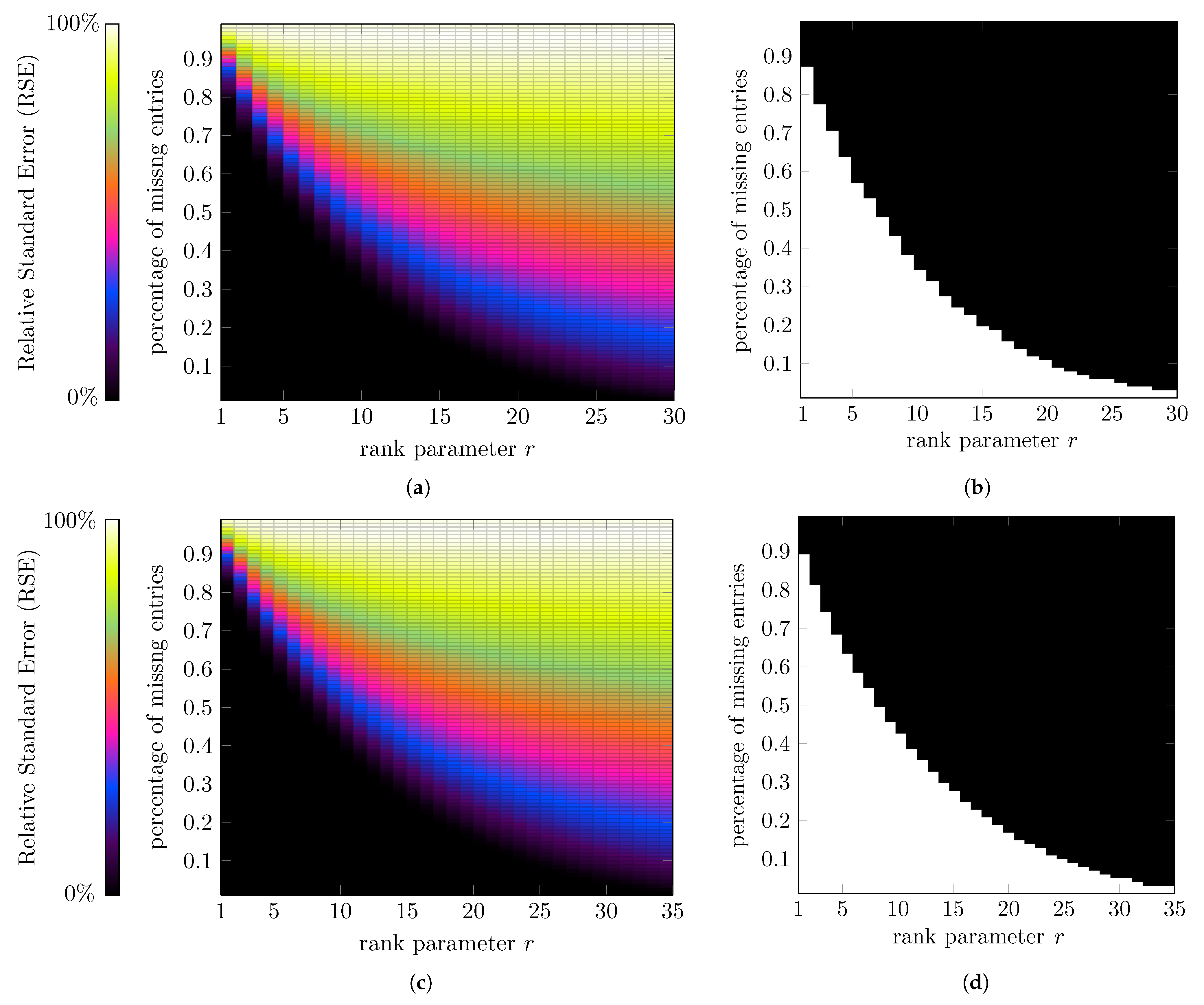
5.1. Experiments on Simulated Random Data

To evaluate the completion capability of the proposed Higher-Order TNN algorithm, we use simulated random t-matrices. Specifically, we generate two random t-matrices P ˙ C D × r and Q ˙ C r × D , which are represented as arrays in R I 1 × I 2 × I 3 × D × r and R I 1 × I 2 × I 3 × r × D , where I 1 × I 2 × I 3 = 3 × 3 × 3 and r < D . The parameter r is (with high probability) the tubal rank as defined by Kilmer et al. [10,25]. The real numbers in the underlying arrays of P ˙ and Q ˙ are independently sampled from the Gaussian distribution N ( 0 , 1 ) .
The product Y ˙ = P ˙ · Q ˙ gives a random t-matrix in C D × D R I 1 × I 2 × I 3 × D × D . The trace rank of Y ˙ is, with high probability, rank trace Y ˙ = I 1 I 2 I 3 · r . From the underlying array of Y ˙ , we randomly and uniformly select entries to simulate missing data. The resulting incomplete Y ˙ , with a varying percentage of missing entries, and a rank parameter r for Y ˙ , serve as inputs to the Higher-Order TNN algorithm.
The Higher-Order TNN algorithm produces a t-matrix X ˙ C D × D R I 1 × I 2 × I 3 × D × D , which is an estimate of Y ˙ . Let · F be the Frobenius norm. If the Relative Standard Error
RSE tensor ( Y ˙ ) tensor ( X ˙ ) F / tensor ( Y ˙ ) F
is less than a threshold, the completion by the Higher-Order TNN algorithm is considered successful.
Figure 2 illustrates the RSE distributions and phase transitions for fifth-order array completions using the proposed Higher-Order TNN. Figure 2a shows the RSE distribution with the parameter D = 40 . Figure 2b shows a phase transition corresponding to D = 50 , where the white and black dots represent successful ( RSE < 1 × 10 2 ) and failed completions, respectively. Figure 2a,c show the RSE distributions with D = 40 and D = 50  Figure 2b,d shows the phase transitions associated with D = 40 and D = 50 , respectively.

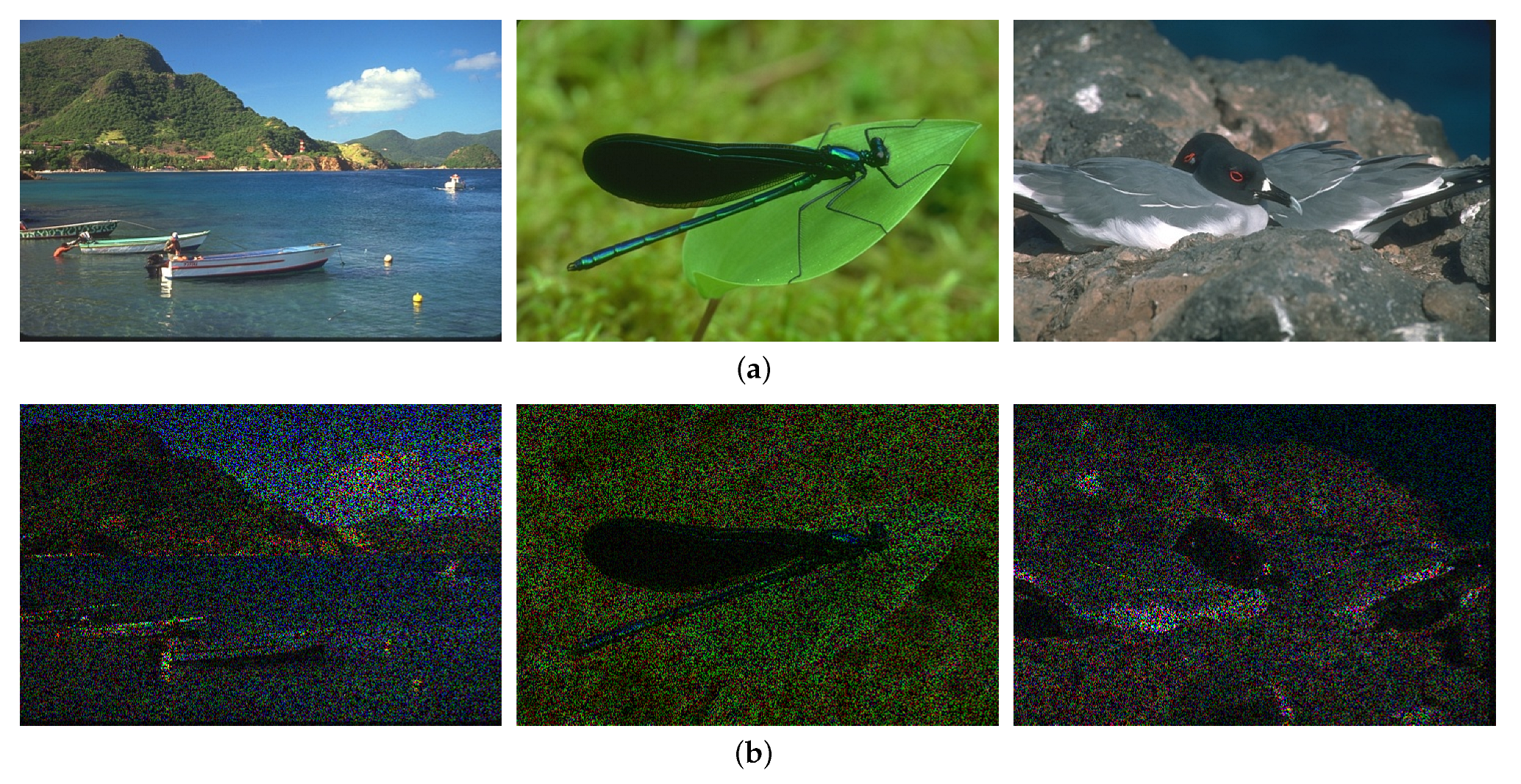
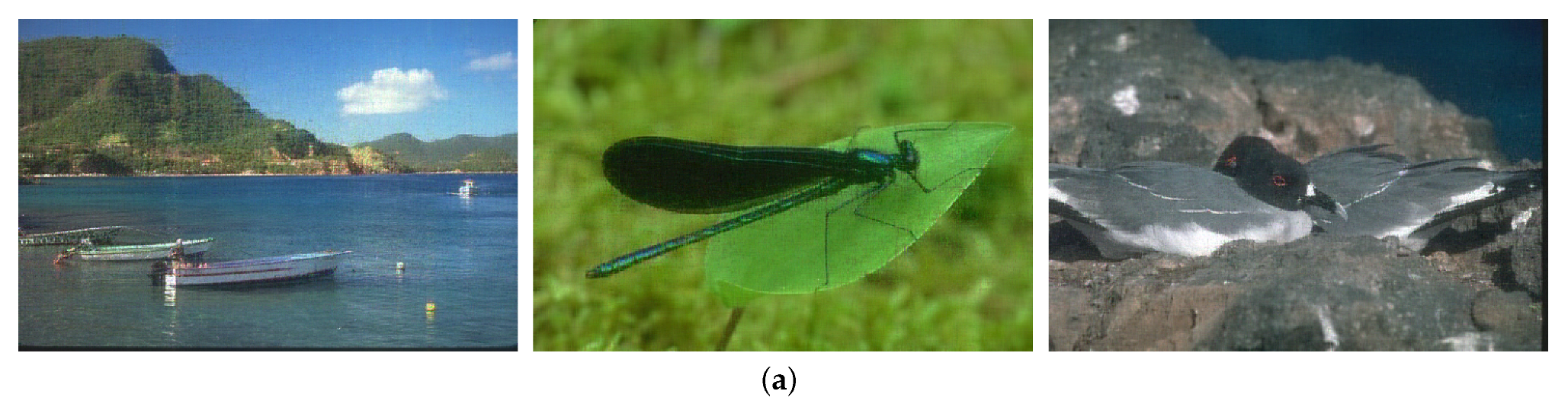
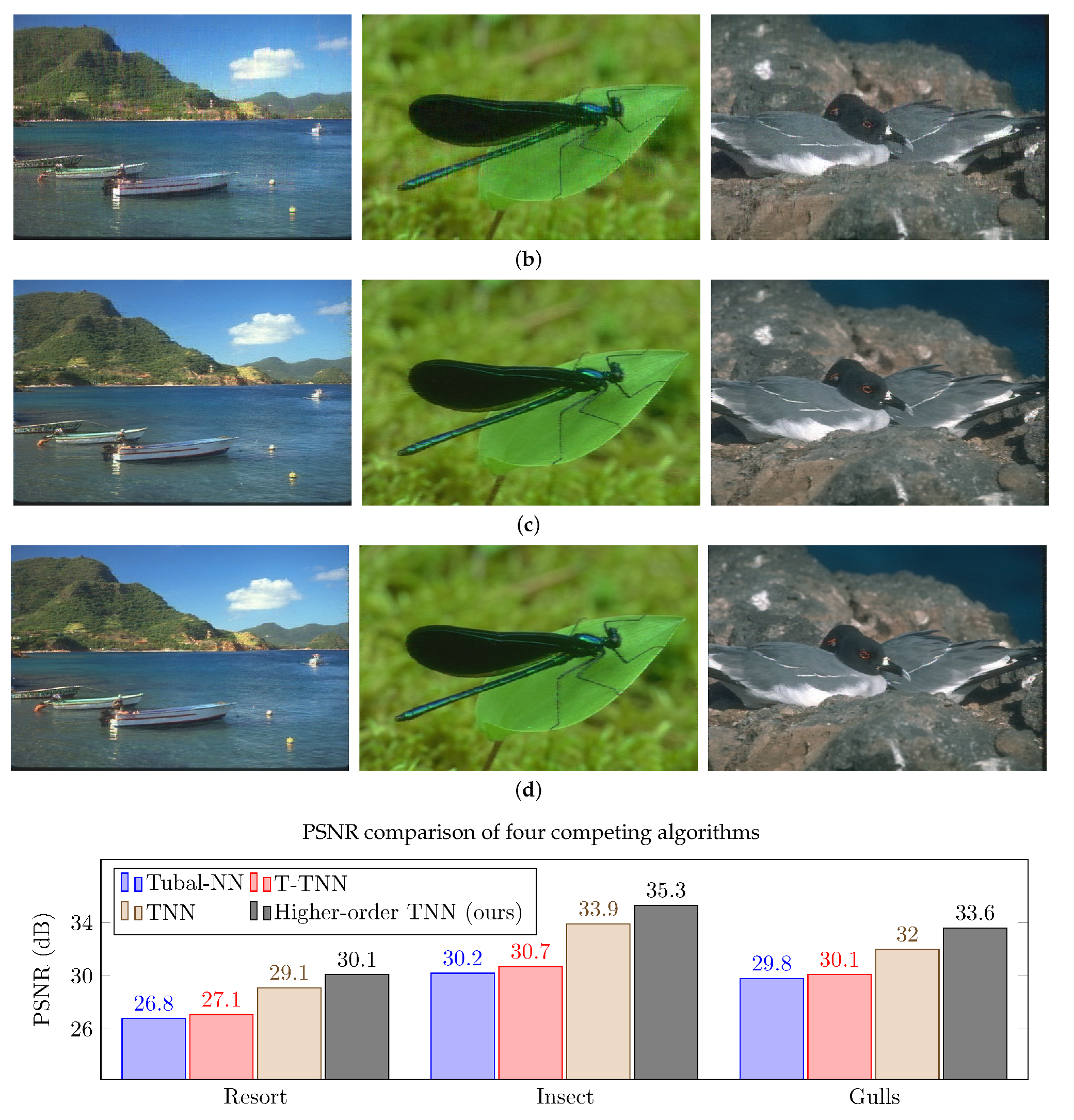
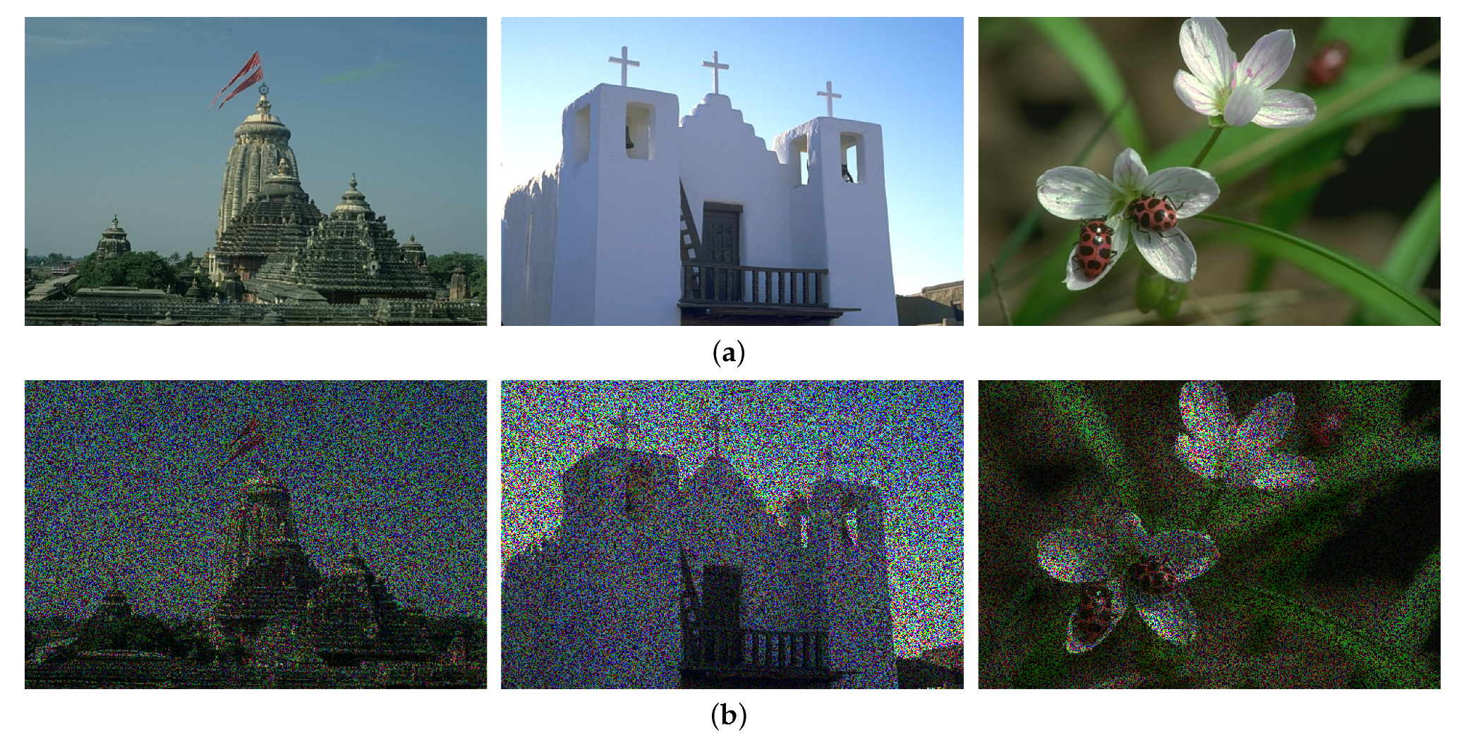
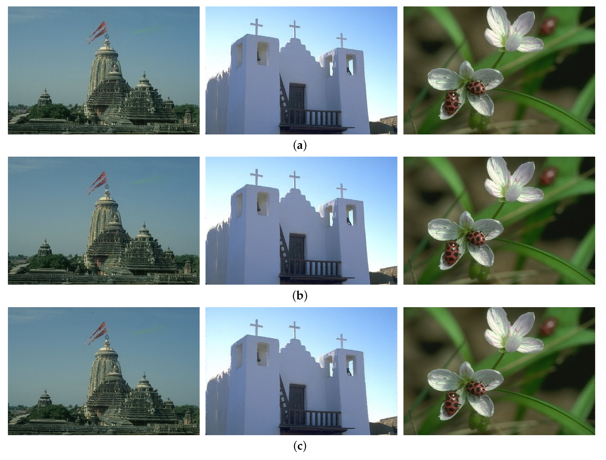
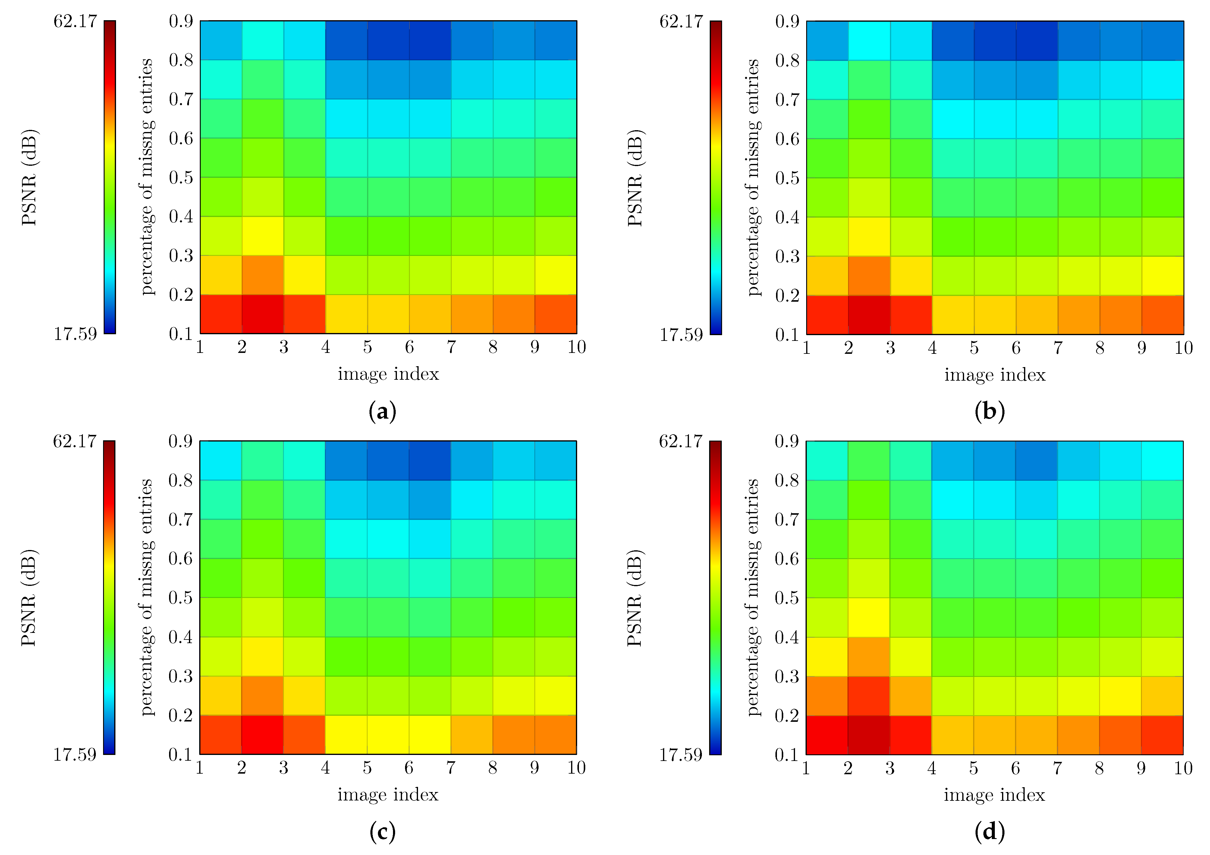
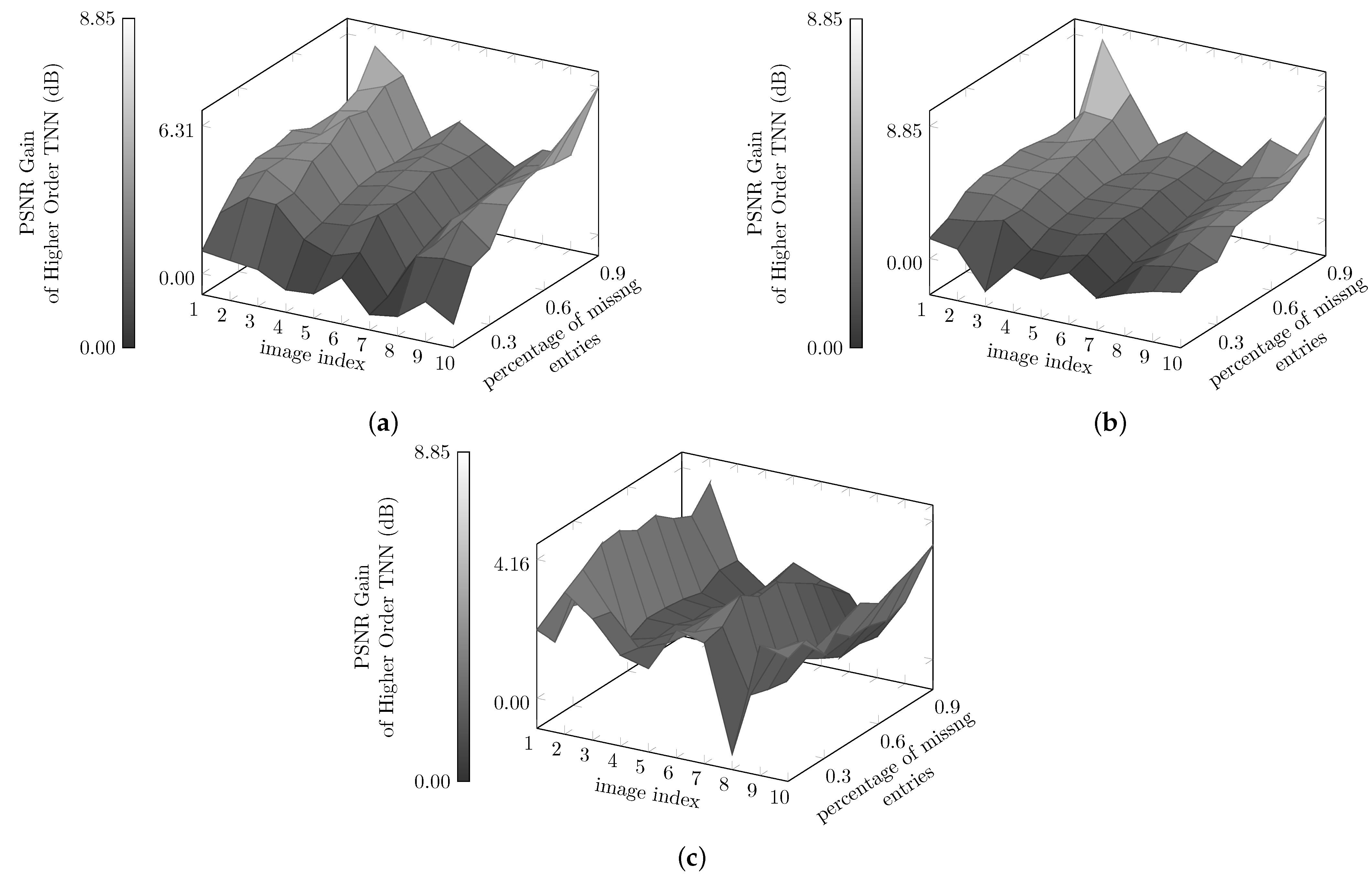
5.2. Experiments on BSD Color Images

In the following experiments, we use the Berkeley Segmentation Dataset as a benchmark to compare the performance of four related algorithms: tubal-TNN [9], T-TNN [12], TNN [11], and our Higher-Order TNN. Three RGB images, namely “Resort”, “Insect”, and “Seagulls”, are selected for the first experiment. These images are represented as 321 × 481 × 3 unsigned integer arrays.
To compare the completion performance, we randomly select 70 % of the pixel values of each image as “missing” entries. The incomplete images, with missing values set to zero, provide a visual representation in Figure 3, which shows the original complete images alongside their incomplete versions.
We use the three competing algorithms and our Higher-Order TNN, described in Algorithm 4, to obtain a complete RGB image of equal size. The quality of the image completion is quantified by the Peak Signal to Noise Ratio (PSNR), defined as
PSNR = 10 · log 10 D 1 · D 2 · D 3 X COMP M F 2
where D 1 · D 2 · D 3 is the number of entries in the RGB image. Note that the entries of X COMP and M are scaled such that the largest entry value in each scaled array is 1.
Figure 4 presents visual and quantitative comparisons of the performance of four competing algorithms in completing the observed images: “Resort”, “Insect”, and “Seagulls” from the Berkeley Segmentation Dataset. The proposed Higher-Order TNN outperforms its competitors in terms of PSNRs by at least 1 dB, 1.4 dB, and 1.6 dB, respectively.
In our second experiment, we use three different images—“Temple”, “Chapel”, and “Grass-flower”, each with 50 % entries randomly missing, to perform completions analogous to the first experiment on the Berkeley images, each with 70 % entries randomly missing. Figure 5 shows the original images along with their incomplete versions.
Figure 6 shows the visual and quantitative comparisons of the four related image completion algorithms. Consistent with the results of the first experiment, the Higher-Order TNN significantly outperforms the other algorithms, achieving gains of at least 1.5 dB, 1.2 dB, and 2.2 dB, respectively.
After experiments on 6 RGB images, our research now includes 10 randomly selected RGB images from the Berkeley Segmentation Dataset, with the percentage of missing entries set to increments within 10 % , 20 % , , 90 % .
Figure 7 shows the 10 randomly selected RGB images used for the experiments. Figure 8 shows the PSNR heatmaps for four relevant algorithms: Tubal-NN [9], T-TNN [12], TNN [11], and our newly developed Higher-Order TNN on the images shown in Figure 7.
These results demonstrate the superior performance of the Higher-Order TNN, as it outperforms its counterparts in terms of PSNR.
For a clearer demonstration, Figure 9 shows the PSNR gains of our Higher-Order TNN over tubal-NN, T-TNN, and TNN. It shows that the PSNR gains of Higher-Order TNN over its counterparts are predominantly positive.

6. Conclusions

In this paper, we consider the problem of higher-order array completion using the higher-order t-matrix model. By adopting a consistent solution, we generalize low-rank matrix completion for the recovery of RGB images with missing entries. Our proposed “Higher-Order TNN” method outperforms competitors such as tubal-TNN, T-TNN, and TNN in terms of recovery performance, demonstrating the ability to exploit higher-order relationships within high-dimensional data and showing advantages.
Our solution not only improves visual data completion, but also paves the way for broader applications. Integrating higher-order generalization into existing systems lays the foundation for more robust and efficient handling of high-order, high-dimensional data. Furthermore, any t-matrix algorithm based on spectral slices of t-matrices has a computational complexity linear in the dimension of the t-algebra. Its independent spectral slices enable faster parallel computation using array programming techniques supported by many programming languages.
We demonstrate this with a generalization of Lu et al.’s [11] tensor completion algorithm to its higher-order version by formulating its matrix model over a finite-dimensional algebra. This is achieved through a novel pixel neighborhood strategy.
The study also provides a consistent methodology for exploring various properties of the t-matrix model, including the notions of rank, norm, and inner product. Compared to the existing “t-product” model, our approach offers new insights into t-scalars and t-matrices from a fresh perspective of representation and operator theory. Moreover, the higher-order Lagrange multiplier with t-matrix variables adds to our contributions.
The inclusion of the novel “trace rank”, nuclear norm, Schatten p-norm, and the adaptation of the recent tensor completion algorithm by Lu et al. for higher-order scenarios highlight our results. The experiments emphasize the competitive advantage of our higher-order matrix completion algorithm in RGB image recovery.

Author Contributions

Author Contributions: Conceptualization, L.L. (Liang Liao) and S.J.M.; methodology, L.L. (Liang Liao); software, Z.G. and Q.G.; validation, L.L. (Liang Liao), Y.W. and F.Y.; formal analysis, L.L. (Liang Liao); investigation, L.L. (Liang Liao), Z.G. and Q.G.; resources, C.L.; data curation, L.L. (Liang Liao), Q.G. and Z.G.; writing—original draft preparation, Z.G. and L.L. (Liang Liao); writing—review and editing, L.L. (Liang Liao) and S.J.M.; visualization, L.L. (Liang Liao), Z.G. and Q.G.; supervision, L.L. (Liang Liao), C.L. and Z.L.; project administration, L.L. (Liang Liao), Q.Z. and L.L. (Lun Li); funding acquisition, L.L. (Liang Liao) and Y.W. All authors have read and agreed to the published version of the manuscript.

Funding

This research was supported by Henan Center for Outstanding Overseas Scientists (No. GZS2020012), “Machine Intelligence and High-Dimensional Data Analysis” Research Team Development program (K2022TD001), and the Key Technologies R&D Program of Henan (Nos. 232102211020, 222102210016).

Data Availability Statement

The original data contributions presented in this study are included in the article.

Conflicts of Interest

The authors declare no conflict of interest.

Appendix A. A Mathematical Justification

The ADMM optimization for low-rank matrix completion described in Algorithm 3 relies on the Lagrange multiplier given in Equation (8). However, the generalized ADMM optimization presented in Algorithm 4 currently lacks a corresponding Lagrange multiplier. To construct a valid Lagrange multiplier, we define a new nuclear norm, a real-valued inner product, and a Frobenius-like norm.

Appendix A.1. Matrix Representation for T-Scalars and Higher-Order Measures

A representation of an algebra C requires a vector space V and a homomorphism from C into End ( V ) , the endomorphism algebra of V.
Each t-scalar in C is represented by a diagonal complex matrix. The diagonal entries of the matrix are the Fourier entries of the t-scalar, resulting in the following mapping for all x ˙ C :
x ˙ M ( x ˙ ) diag F 1 ( x ˙ ) , , F K ( x ˙ ) .
Here, F 1 ( x ˙ ) , , F K ( x ˙ ) represent the Fourier entries of F ( x ˙ ) .
It is obvious that F 1 ( x ˙ ) , , F K ( x ˙ ) are eigenvalues of both the t-scalar x ˙ and the matrix M ( x ˙ ) . The conjugate x ˙ * maps to the conjugate transpose M ( x ˙ ) H of M ( x ˙ ) . The following mapping is one-to-one.
x ˙ * M ( x ˙ ) H = diag F 1 ( x ˙ ) ¯ , , F K ( x ˙ ) ¯ .
Since any t-scalar x ˙ is a normal operator, i.e., x ˙ * x ˙ = x ˙ x ˙ * , there exists a unique non-negative square root | x ˙ | x ˙ * x ˙ , which leads to the following one-to-one mapping:
| x ˙ | diag | F 1 ( x ˙ ) | , , | F K ( x ˙ ) | .
In operator theory, such a non-negative square root is called a positive operator, alternatively a “non-negative operator”, by Definition 5, despite its less common usage. This non-negative operator (t-scalar) can appropriately be called the higher-order absolute value of x ˙ .
In addition, a t-scalar behaves as an endomorphism within the finite-dimensional algebra C and as such has a trace. The trace of any given t-scalar x ˙ can be computed via
trace ( x ˙ ) = F 1 ( x ˙ ) + + F K ( x ˙ ) .
This trace, when pertaining to a non-negative t-scalar (a non-negative operator), is a non-negative real number. This property elevates the partial order of non-negative t-scalars to a total order. Therefore, the trace of the higher-order absolute value x ˙ * x ˙ , or the trace norm of x ˙ C , can be determined.
The trace norm of a t-scalar is the nuclear norm of its matrix representation. For any t-scalar x ˙ , this relation can be expressed as
trace | x ˙ | trace M | x ˙ | = M ( x ˙ ) * , x ˙ C .
Equation (A5) implies that the norm of M ( x ˙ ) serves as a real-valued, totally ordered amplitude of x ˙ . Together with M ( x ˙ ) * , the Schatten 2-norm M ( x ˙ ) 2 is also a valid norm of x ˙ . However, due to the non-isometric nature of the Fourier transform, M ( x ˙ ) 2 is not equal to the Frobenius norm tensor ( x ˙ ) F .
The non-negative t-scalar | x ˙ | x ˙ * x ˙ fully encompasses the amplitude information of the t-scalar x ˙ . Both the Schatten 2-norm and the Frobenius norm of the underlying tensor of x ˙ can be derived from | x ˙ | as follows:
M ( x ˙ ) 2 = K · tensor ( x ˙ ) F = trace | x ˙ | .
where K is the dimension of the algebra C.

Appendix A.2. A Representation Model for T-Matrices and Higher-Order Measures

Consider a t-matrix X ˙ C D 1 × D 2 , characterized by its higher-order singular values σ ˙ 1 σ ˙ 2 σ ˙ n z ˙ . The higher order Schatten p-norm of X ˙ is defined by
N p ( X ˙ ) = n σ ˙ n p 1 / p z ˙ .
A t-matrix X ˙ C D 1 × D 2 can be represented by placing the diagonal matrix of each corresponding t-scalar into its respective block in the final matrix. If the diagonal matrix size of a t-scalar is K × K , then the matrix representation of X ˙ is C K D 1 × K D 2 , as shown by Liao et al. [33].
However, matrix representations are not unique. In addition to the above format, a more convenient representation uses the direct sum of matrices, also known as the block diagonal sum. This operation combines several matrices into a larger one, where the summand matrices are arranged along the main diagonal and off-diagonal blocks are filled with zeros. In this appendix, we stick to this representation in the direct sum of matrices.
Given a t-matrix X ˙ C D 1 × D 2 with spectral slices denoted by X ˜ 1 , , X ˜ K , the direct sum representation of X ˙ is established via a bijective mapping:
X ˙ M ( X ˙ ) X ˜ 1 X ˜ 2 X ˜ K X ˜ 1 0 0 0 X ˜ 2 0 0 0 X ˜ K .
This mapping extends the bijective mapping for t-scalars given in Equation (A1). Kilmer et al. [10,25] proposed the first version of this mapping for the analysis of t-matrices with order-one entries.
It is easy to see that X ˙ * M ( X ˙ ) H = k = 1 K X ˜ k H . Furthermore, given the one-to-one nature of the mapping, we can define the rank of X ˙ by the rank of M ( X ˙ ) , which leads to the following equation:
rank X ˙ rank M ( X ˙ ) = k = 1 K rank X ˜ k .
This definition corresponds to the “trace rank” discussed in Section 4.2. The direct sum representation also provides a mathematical justification for Algorithm 1. In particular, if the singular value decomposition of the summand X ˜ k is X ˜ k = U k · S k · V k H , the following equation of direct sums holds for all X ˙ ,
k = 1 K X ˜ k = k = 1 K U k · S k · V k H = k = 1 K U k · k = 1 K S k · k = 1 K V k H .
In addition, the following equation is obtained from the TSVD of X ˙ :
X ˙ = M 1 k = 1 K U k M 1 k = 1 K S k M * k = 1 K V k
where M * ( · ) is a shorthand for ( M 1 ( · ) ) * .

Appendix A.3. Lagrange Multiplier with T-Matrix Variables

The direct sum properties also validate the spectral-slice-wise mechanism exhibited in Algorithms 2–4. We present a generalized version of Equation (8). The Lagrange multiplier with t-matrix variables has the following form:
L ( X ˙ , E ˙ , Y ˙ , τ ) = X ˙ * + Y ˙ , M ˙ X ˙ E ˙ + 1 2 τ M ˙ X ˙ E ˙ 2 2 .
The real-valued Schatten 2-norm X ˙ 2 can also be derived from the higher-order Schatten 2-norm N p ( X ˙ ) given in Equation (A7). Consequently, for all t-matrices X ˙ , the following equation holds:
X ˙ 2 M ( X ˙ ) 2 = trace N 2 ( X ˙ ) 2 0 .
It is important to note that X ˙ 2 is measured by spectral slices and the Fourier transform is not isometric. Therefore, unlike the case for conventional matrices, the Schatten 2-norm X ˙ 2 and the Frobenius norm tensor ( X ˙ ) F are different. For any t-matrix X ˙ , the equality X ˙ 2 = K · tensor ( X ˙ ) F holds.
Similarly, the nuclear norm of any t-matrix X ˙ is defined by the nuclear norm of M ( X ˙ ) . As with the Schatten 2-norm, the real-valued nuclear norm X ˙ * can be derived from its higher-order counterpart N 1 ( X ˙ ) as follows:
X ˙ * M ( X ˙ ) * = trace N 1 ( X ˙ ) .
Currently, a real inner product X ˙ , Y ˙ of a pair of t-matrices X ˙ , Y ˙ is required to have the full Lagrange multiplier as in Equation (A12). However, if the inner product X ˙ , Y ˙ is defined as trace M ( X ˙ ) H M ( Y ˙ ) , it will be complex.
To ensure a real-valued inner product instead of a complex-valued one, a feasible strategy is to map M ( X ˙ ) to a real matrix for any t-matrix X ˙ .
According to representation theory, any complex number a + b 1 can be represented as a 2 × 2 real matrix using the following mapping:
a + b 1 a b b a .
By replacing each complex entry of M ( X ˙ ) C K D 1 × K D 2 with its 2 × 2 real matrix equivalent, the complex matrix M ( X ˙ ) C K D 1 × K D 2 can be isomorphically transformed into a real matrix R ( X ˙ ) R 2 K D 1 × 2 K D 2 . Thus, the real inner product for any pair of t-matrices X ˙ and Y ˙ can be defined as
X ˙ , Y ˙ ( 1 / 2 ) · trace R ( X ˙ ) T R ( Y ˙ ) .
The coefficient ( 1 / 2 ) is essential to account for the doubling of absolute values in the real representation.
The following required investigation is standard in convex analysis with the Lagrange multiplier given by Equation (A12) and has been studied extensively by previous authors. Therefore, it is beyond the scope of this appendix.

References

  1. Floryan, D.; Graham, M.D. Data-driven discovery of intrinsic dynamics. Nat. Mach. Intell. 2022, 4, 1113–1120. [Google Scholar] [CrossRef]
  2. Li, T.; Tan, L.; Huang, Z.; Tao, Q.; Liu, Y.; Huang, X. Low dimensional trajectory hypothesis is true: DNNs can be trained in tiny subspaces. IEEE Trans. Pattern Anal. Mach. Intell. 2022, 45, 3411–3420. [Google Scholar] [CrossRef]
  3. Chen, M.; Jiang, H.; Liao, W.; Zhao, T. Nonparametric regression on low-dimensional manifolds using deep ReLU networks: Function approximation and statistical recovery. Inf. Inference J. IMA 2022, 11, 1203–1253. [Google Scholar] [CrossRef]
  4. Xu, Y.; Yu, Z.; Cao, W.; Chen, C.L.P. A novel classifier ensemble method based on subspace enhancement for high-dimensional data classification. IEEE Trans. Knowl. Data Eng. 2021, 35, 16–30. [Google Scholar] [CrossRef]
  5. Fu, L.; Yang, J.; Chen, C.; Zhang, C. Low-rank tensor approximation with local structure for multi-view intrinsic subspace clustering. Inf. Sci. 2022, 606, 877–891. [Google Scholar] [CrossRef]
  6. Wang, M.; Wang, Q.; Hong, D.; Roy, S.K.; Chanussot, J. Learning tensor low-rank representation for hyperspectral anomaly detection. IEEE Trans. Cybern. 2022, 53, 679–691. [Google Scholar] [CrossRef]
  7. Liu, N.; Li, W.; Wang, Y.; Tao, R.; Du, Q.; Chanussot, J. A survey on hyperspectral image restoration: From the view of low-rank tensor approximation. Sci. China Inf. Sci. 2023, 66, 140302. [Google Scholar] [CrossRef]
  8. Liu, J.; Musialski, P.; Wonka, P.; Ye, J. Tensor Completion for Estimating Missing Values in Visual Data. IEEE Trans. Pattern Anal. Mach. Intell. 2012, 35, 208–220. [Google Scholar] [CrossRef]
  9. Zhang, Z.; Ely, G.; Aeron, S.; Hao, N.; Kilmer, M. Novel methods for multilinear data completion and de-noising based on tensor-SVD. In Proceedings of the IEEE Conference on Computer Vision and Pattern Recognition, Columbus, OH, USA, 23–28 June 2014; pp. 3842–3849. [Google Scholar]
  10. Kilmer, M.E.; Martin, C.D. Factorization strategies for third-order tensors. Linear Algebra Its Appl. 2011, 435, 641–658. [Google Scholar] [CrossRef]
  11. Lu, C.; Feng, J.; Lin, Z.; Yan, S. Exact low tubal rank tensor recovery from Gaussian measurements. arXiv 2018, arXiv:1806.02511. [Google Scholar]
  12. Xue, S.; Qiu, W.; Liu, F.; Jin, X. Low-rank tensor completion by truncated nuclear norm regularization. In Proceedings of the 2018 24th IEEE International Conference on Pattern Recognition (ICPR), Beijing, China, 20–24 August 2018; pp. 2600–2605. [Google Scholar]
  13. Zeng, H.; Xue, J.; Luong, H.Q.; Philips, W. Multimodal core tensor factorization and its applications to low-rank tensor completion. IEEE Trans. Multimed. 2022; early access. [Google Scholar] [CrossRef]
  14. Wu, Z.; Huang, T.; Deng, L.; Dou, H.; Meng, D. Tensor wheel decomposition and its tensor completion application. Adv. Neural Inf. Process. Syst. 2022, 35, 27008–27020. [Google Scholar]
  15. Zhao, X.; Bai, M.; Sun, D.; Zheng, L. Robust tensor completion: Equivalent surrogates, error bounds, and algorithms. SIAM J. Imaging Sci. 2022, 15, 625–669. [Google Scholar] [CrossRef]
  16. Deng, L.; Xiao, M. A New Automatic Hyperparameter Recommendation Approach Under Low-Rank Tensor Completion e Framework. IEEE Trans. Pattern Anal. Mach. Intell. 2022, 45, 4038–4050. [Google Scholar] [CrossRef]
  17. Nguyen, T.; Uhlmann, J. Tensor completion with provable consistency and fairness guarantees for recommender systems. ACM Trans. Recomm. Syst. 2023, 1, 1–26. [Google Scholar] [CrossRef]
  18. Hui, B.; Yan, D.; Chen, H.; Ku, W.-S. Time-sensitive POI Recommendation by Tensor Completion with Side Information. In Proceedings of the 2022 IEEE 38th International Conference on Data Engineering (ICDE), Kuala Lumpur, Malaysia, 9–12 May 2022; pp. 205–217. [Google Scholar]
  19. Song, Q.; Ge, H.; Caverlee, J.; Hu, X. Tensor completion algorithms in big data analytics. ACM Trans. Knowl. Discov. Data 2019, 13, 1–48. [Google Scholar] [CrossRef]
  20. Wu, X.; Xu, M.; Fang, J.; Wu, X. A multi-attention tensor completion network for spatiotemporal traffic data imputation. IEEE Internet Things J. 2022, 9, 20203–20213. [Google Scholar] [CrossRef]
  21. Lee, C.; Wang, M. Beyond the signs: Nonparametric tensor completion via sign series. Adv. Neural Inf. Process. Syst. 2021, 34, 21782–21794. [Google Scholar]
  22. Liao, L.; Maybank, S.J. Generalized visual information analysis via tensorial algebra. J. Math. Imaging Vis. 2020, 62, 560–584. [Google Scholar] [CrossRef]
  23. Chang, S.Y.; Wei, Y. T-product tensors—Part II: Tail bounds for sums of random T-product tensors. Comput. Appl. Math. 2022, 41, 99. [Google Scholar] [CrossRef]
  24. Yu, Q.; Zhang, X. T-product factorization based method for matrix and tensor completion problems. Comput. Optim. Appl. 2022, 84, 761–788. [Google Scholar] [CrossRef]
  25. Kilmer, M.E.; Braman, K.; Hao, N.; Hoover, R.C. Third-order tensors as operators on matrices: A theoretical and computational framework with applications in imaging. SIAM J. Matrix Anal. Appl. 2021, 34, 148–172. [Google Scholar] [CrossRef]
  26. Lim, L.-H. Tensors and Hypermatrices, Handbook of Linear Algebra (Leslie Hogben, Ed.); CRC Press: Boca Raton, FL, USA, 2013. [Google Scholar]
  27. Candès, E.J.; Li, X.; Ma, Y.; Wright, J. Robust principal component analysis? J. ACM (JACM) 2021, 58, 1–37. [Google Scholar] [CrossRef]
  28. Candès, E.; Recht, B. Exact matrix completion via convex optimization. Commun. ACM 2012, 55, 111–119. [Google Scholar] [CrossRef]
  29. Lin, Z.; Li, H.; Fang, C. Alternating Direction Method of Multipliers for Machine Learning; Springer: Berlin/Heidelberg, Germany, 2022. [Google Scholar]
  30. Han, D.-R. A survey on some recent developments of alternating direction method of multipliers. J. Oper. Res. Soc. China 2022, 10, 1–52. [Google Scholar] [CrossRef]
  31. Lu, C.; Feng, J.; Chen, Y.; Liu, W.; Lin, Z.; Yan, S. Tensor robust principal component analysis with a new tensor nuclear norm. IEEE Trans. Pattern Anal. Mach. Intell. 2019, 42, 925–938. [Google Scholar] [CrossRef]
  32. Liao, L.; Maybank, S.J. General data analytics with applications to visual information analysis: A provable backward-compatible semisimple paradigm over t-algebra. arXiv 2020, arXiv:2011.00307. [Google Scholar]
  33. Liao, L.; Lin, S.; Li, L.; Zhang, X.; Zhao, S.; Wang, Y.; Wang, X.; Gao, Q.; Wang, J. Approximation of Images via Generalized Higher Order Singular Value Decomposition over Finite-Dimensional Commutative Semisimple Algebra. arXiv 2022, arXiv:2202.00450. [Google Scholar]
Figure 1. Elevating a 4 × 4 grayscale image to a fourth-order array using a central 3 × 3 pixel neighborhood strategy.
Axioms 12 00954 g001
Figure 2. RSE distributions and phase transitions (threshold RSE = 1 × 10 2 ) of Higher-Order TNN, with D = 40 and 50. (a) RSE distribution, D = 40 . (b) phase transition, D = 40 . (c) RSE distribution, D = 50 . (d) phase transition, D = 50 .
Axioms 12 00954 g002
Figure 3. Three original and observed images: “Resort”, “Insect”, and “Seagulls” from the Berkeley Segmentation Dataset. (a) Original images. (b) Observed images with missing 70 % entries.
Axioms 12 00954 g003
Figure 4. Visual and quantitative comparisons of the performance of four related algorithms in completing the images “Resort”, “Insect”, and “Seagulls”. (a) Tubal-NN [9]. (b) T-TNN [12]. (c) TNN [11]. (d) Higher-Order TNN (ours).
Axioms 12 00954 g004aAxioms 12 00954 g004b
Figure 5. Three original and observed images: “Temple”, “Chapel”, and “Grass-flower” from the Berkeley Segmentation Dataset. (a) Orignal images. (b) Observed images with 50 % entries missing.
Axioms 12 00954 g005
Figure 6. Visual and quantitative comparisons of the performance of four related algorithms in completing the images “Temple”, “Chapel”, and “Grass-flower”. (a) Tubal-NN [9]. (b) T-TNN [12]. (c) TNN [11]. (d) Higher-Order TNN (ours).
Axioms 12 00954 g006aAxioms 12 00954 g006b
Figure 7. 10 random RGB images selected from the Berkeley Segmentation Dataset.
Axioms 12 00954 g007
Figure 8. PSNR heatmaps of four algorithms with different percentages of missing entries on 10 RGB images. (a) Tubal-NN [9]. (b) T-TNN [12]. (c) TNN [11]. (d) Higher-Order TNN (ours).
Axioms 12 00954 g008
Figure 9. Higher-Order TNN’s PSNR gains over its competitors. (a) PSNR gain over tubal-TNN. (b) PSNR gain over T-TNN. (c) PSNR gain over TNN.
Axioms 12 00954 g009
Disclaimer/Publisher’s Note: The statements, opinions and data contained in all publications are solely those of the individual author(s) and contributor(s) and not of MDPI and/or the editor(s). MDPI and/or the editor(s) disclaim responsibility for any injury to people or property resulting from any ideas, methods, instructions or products referred to in the content.

