Article

A Modified Quantum-Inspired Genetic Algorithm Using Lengthening Chromosome Size and an Adaptive Look-Up Table to Avoid Local Optima

1
Department of Computer Engineering, Mashhad Branch, Islamic Azad University, Mashhad 9187147578, Iran
2
Department of Electrical Engineering, Mashhad Branch, Islamic Azad University, Mashhad 9187147578, Iran
3
School of Business, University of Southern Queensland, Toowoomba 4350, Australia
*
Author to whom correspondence should be addressed.
Submission received: 9 August 2023 / Revised: 21 September 2023 / Accepted: 26 September 2023 / Published: 17 October 2023
(This article belongs to the Special Issue Computational Aspects of Machine Learning and Quantum Computing)

Abstract

:
The quantum-inspired genetic algorithm (QGA), which combines quantum mechanics concepts and GA to enhance search capability, has been popular and provides an efficient search mechanism. This paper proposes a modified QGA, called dynamic QGA (DQGA). The proposed algorithm utilizes a lengthening chromosome strategy for a balanced and smooth transition between exploration and exploitation phases to avoid local optima and premature convergence. Apart from that, a novel adaptive look-up table for rotation gates is presented to boost the algorithm’s optimization abilities. To evaluate the effectiveness of these ideas, DQGA is tested by various mathematical benchmark functions as well as real-world constrained engineering problems against several well-known and state-of-the-art algorithms. The obtained results indicate the merits of the proposed algorithm and its superiority for solving multimodal benchmark functions and real-world constrained engineering problems.

1. Introduction

Metaheuristic optimization algorithms have been proposed to tackle complex, high-dimensional problems without comprehensive knowledge of the problem’s nature and their search spaces’ derivative information, which is essential for finding critical points of the search space in classical optimization methods. Metaheuristics have the ability to treat optimization problems as black boxes. So, the input, output, and a proper fitness function of an optimization problem suffice to solve the problem. As a result, metaheuristic algorithms are problem-independent, meaning they can be applied to a wide variety of problems with subtle modifications. Metaheuristic algorithms provide acceptable results in a timely manner for many real-world optimization problems, but their computational cost is excessively high using conventional algorithms. Some examples of the applications are image and signal processing [1], engineering and structural design [2], routing problems [3], feature selection [4], stock market portfolio optimization [5], RNA prediction [6], and resource management problems [7].
Han and Kim proposed the prominent genetic quantum algorithm (GQA) [8] and the quantum-inspired evolutionary algorithm [9] for combinatorial optimization problems using qubit representation and quantum rotation gates instead of the ‘crossover’ operator, in the genetic algorithm (GA). The probabilistic representation of qubits used in quantum-inspired metaheuristic optimization algorithms instead of bits expands the diversity of individuals in the algorithm’s population, so it helps the optimization algorithm avoid premature convergence and getting stuck in local optima. Recently, a relatively large number of quantum-inspired metaheuristics have been proposed to solve a vast range of real-world optimization problems. Some recent examples are as follows. In [10,11,12], quantum-inspired metaheuristics are applied to image processing problems, and structural design applications are presented in [13,14,15,16]. In  [17,18,19,20,21,22], quantum-inspired metaheuristics are utilized for job-scheduling problems, and some examples of network applications of quantum-inspired metaheuristics are found in [23,24,25,26]. In [27], a quantum-inspired metaheuristic is used for quantum circuit synthesis. Other applications are feature selection [28,29], fuzzy c-means clustering [30], stock market portfolio optimization [31], flight control optimization [32,33], antenna positioning problems [34], airport gate allocation [35], and multi-objective optimization [36]. A comprehensive review of quantum-inspired metaheuristics and their variants is presented in [37,38]. Considering the diverse range of applications of quantum-inspired metaheuristics, it is clear that this scope has gained much attention, and this approach can solve real-world optimization problems effectively.
Metaheuristic optimization algorithms such as GA [39] have been widely used in solving some important optimization problems in, e.g., the field of quantum information and computation, such as in distributed quantum computing [40,41,42,43], in the design and the optimization of quantum circuits [44,45,46], and in finding stabilizers of a given sub-space [47], etc.
The main challenge in all metaheuristic algorithms is achieving a properly balanced transition between the exploration and exploitation phases. This paper proposed DQGA to establish a smooth transition between the exploration and exploitation phases. The principal objective of the proposed algorithms is to boost global search ability without deteriorating the local search.
DQGA enhances the search power of QGA with two contributions:
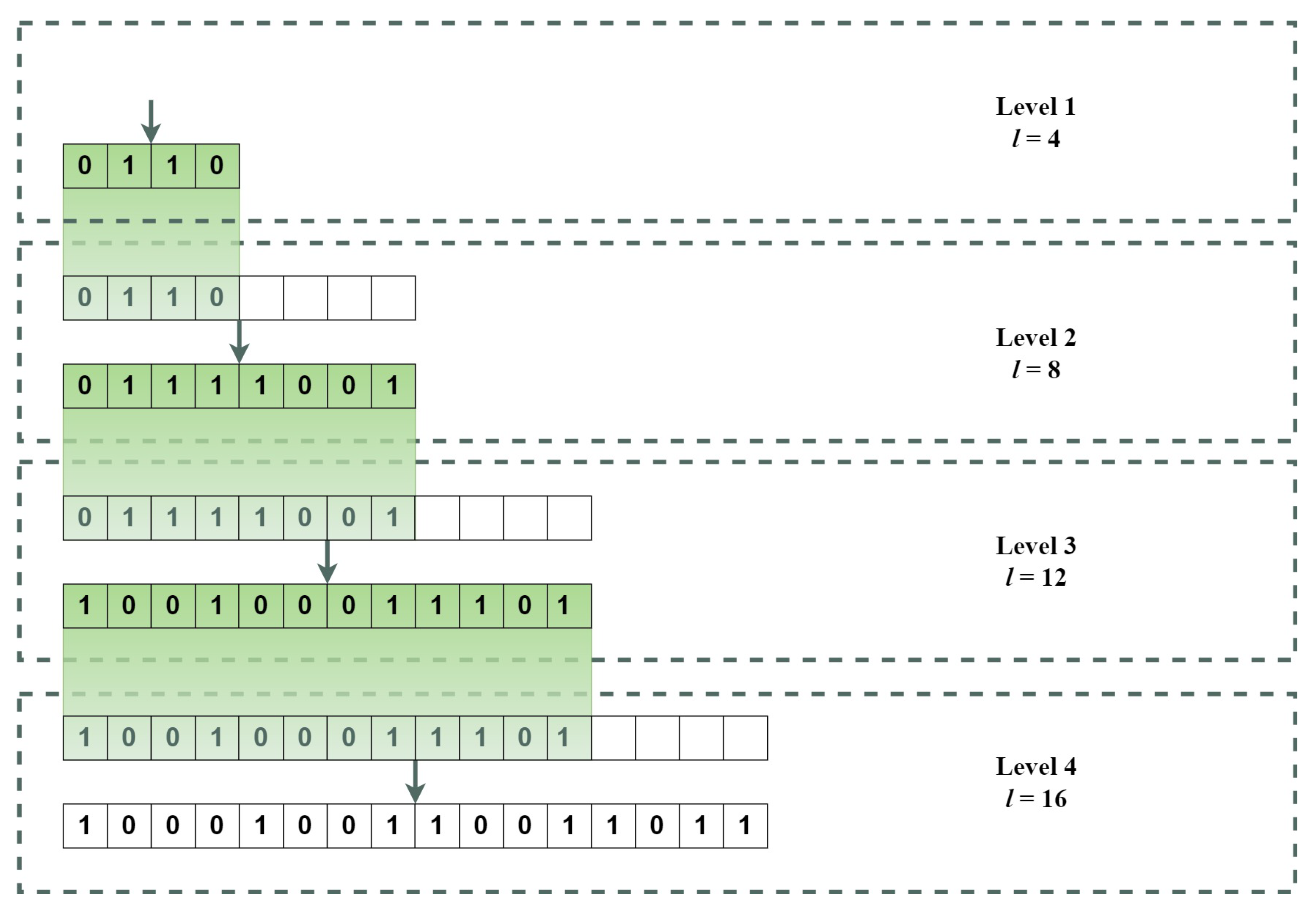
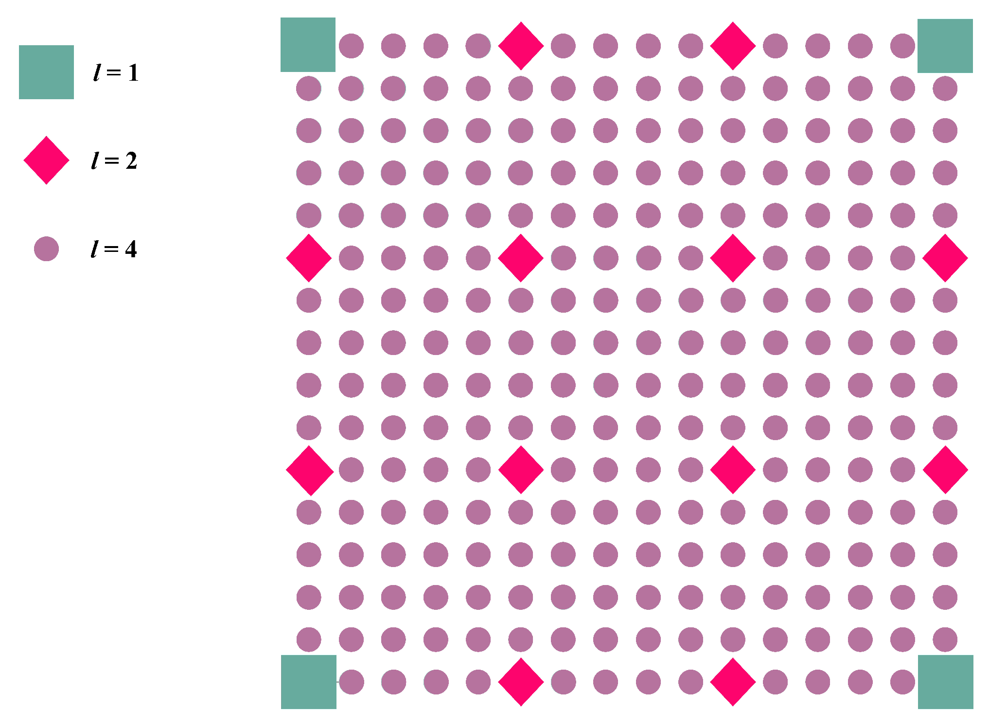
  • Lengthening Chromosomes Size: DQGA increases the size of chromosomes throughout the algorithm run. This strategy leads to increasing precision levels for the duration of generations. Low precision levels for early generations cause higher global focus and less attention to detail, favoring diversification. As opposed to that, higher precision in the last generations promotes intensification. This manner guarantees a smooth shift from the exploration phase to the exploitation phase. It should be noted that the concept of utilizing variable chromosome size was introduced in [48] as an attempt to find a suitable chromosome size for reducing computational time. Also, in [49], the authors used different chromosome sizes to cover diverse coarse-grained and fine-grained parts of a design in topological order. However, in this paper, we utilized incrementing chromosome size for different purposes, namely local optima and premature convergence avoidance.
  • Adaptive Rotation Steps: Unlike the look-up table of the original GQA, which consists of fixed values for all generations and ignores the current state of the qubits, the proposed DQGA uses an adaptive look-up table which helps the algorithm to search more properly and improves the exploration–exploitation transition.
The rest of this paper is structured as follows. Section 2 presents the quantum computing basics and an overview of GQA. The proposed DQGA algorithm is described in Section 3. The results and the comparisons of the performance of the proposed algorithm on benchmark functions and real-world engineering optimization problems are given in Section 4, as well as the comparison of the results with well-known metaheuristic algorithms. Finally, Section 5 concludes this work and points out future studies.

2. Fundamentals

2.1. Quantum Computing Basics

Like bits in classical processing are the basic units of information, quantum bits, or qubits, are the units of information in quantum computing. The mathematical representation of a qubit is a unit vector in a two-dimensional Hilbert space for which the basis vectors are denoted by the symbols 0 and 1 . Unlike classical bits, qubits can be in the superposition of 0 and 1 like α 0 + β 1 , where α and β are complex numbers such that | α 2 | + | β 2 | = 1 .
If the qubit is measured in the computational, i.e., { 0 , 1 } basis, the classic outcome of 0 is observed with the probability of | α | 2 and the classic outcome of 1 is observed with the probability of | β | 2 . If 0 is observed, the state of the qubit after the measurement collapses to 0 , otherwise, it collapses to 1  [50].
A register with m qubits is defined as:
α 1 α 2 α m β 1 β 2 β m , i { 1 , , m } , | α i | 2 + | β i | 2 = 1 .
An m-qubit register is able to represent 2 m states simultaneously. The probability of collapsing into each of these 2 m states after measurement is the multiplication of the corresponding probability amplitudes squared [40]. For example, consider a system comprised of three qubits as follows:
2 2 3 2 2 2 2 2 1 2 2 2 .
The state of the system can be described as:
3 4 000 + 3 4 001 + 1 4 010 + 1 4 011 + 3 4 100 + 3 4 101 + 1 4 110 + 1 4 111 ,
which means the probabilities for the system to represent the states 000 , 001 , 010 , 011 , 100 , 101 , 110 , and  111 are 3 16 , 3 16 , 1 16 , 1 16 , 3 16 , 3 16 , 1 16 , and  1 16 , respectively.
Manipulation of qubits is performed through quantum gates. A quantum gate is a linear transformation and is reversible. A unitary matrix U is used to define a quantum gate. A complex square matrix U is unitary if its conjugate transpose U and its inverse U 1 are the same. So for any unitary matrix U Equation (4) holds.
U U = U U = I .

2.2. GQA

The canonical QGA called GQA is presented by Han and Kim [8]. GQA is similar to its conventional counterpart GA in terms of being population-based and evolving a set of generations. Still, it differs from GA because it uses quantum rotation gates instead of the classical crossover operator. The probabilistic nature of qubit representation made the mutation operator expendable, so there is no mutation operator in GQA.
Just like its ancestor, QGA uses a population of individuals to become evolved through the generations, but unlike GA, the individuals consist of qubits instead of bits in GQA. The population at generation t is defined as:
Q ( t ) = { q 1 t q 2 t , q n t } ,
where n is the population size and q j t is a qubit chromosome and is defined by Equation (6),
q j t = α 1 t α 2 t α m t β 1 t β 2 t β m t ,
where m is the chromosome size and j = 1 , 2 , . . . , n . Updating qubits through the quantum rotation gate is visually illustrated in Figure 1 and is mathematically presented in Equation (7). To give an equal chance for all qubits to be measured into 0 and 1 , they are initialized by 1 2 .
α i β i = cos Δ θ i sin Δ θ i sin Δ θ i cos Δ θ i α i β i ,
where Δ θ i is the rotation angle and α i and β i are the probability amplitudes of the qubit after being updated. In each generation, the quantum rotation gates push the qubit population to be more likely to collapse into the best individual state.
It is worth mentioning that quantum gates are susceptible to noise that can affect the measurements for real quantum computer implementation of quantum-inspired metaheuristic optimization algorithms. However, because of the stochastic nature of metaheuristics, it is not necessarily a drawback. In fact, the noise in quantum gates can play the role of the mutation operator in conventional GA, as it randomly changes the state of qubits with a small probability, leading to further diversity in the population.

3. DQGA

In this section, DQGA is presented. The algorithm uses a lengthening chromosome size strategy and an adaptive look-up table to determine quantum rotation gates. As the algorithm works on different levels (i.e., different chromosome sizes), the whole number of generations should be appropriately distributed among the levels. So, we introduced a generation distribution scheme to maximize the algorithm’s performance in the given number of generations. The pseudo-code of DQGA is given in Algorithm 1, and  Figure 2 presents the flowchart of the algorithm. We will explain these concepts in detail in the following subsections.

3.1. Lengthening Chromosome Size Strategy

The lengthening chromosome size strategy enables the chromosomes of the algorithm to grow longer as the generations pass. This algorithm behavior guarantees a balanced transition between the exploration and exploitation phases. The algorithm starts with short-length chromosomes, which yield answers with low precision. At each level of the precision, the previous level best individual becomes the current level best individual and leads the population to previously found promising areas of the search space.
An example of this procedure is depicted in Figure 3. It shows an instance of a four-level run of the algorithm. The chromosome size on levels 1 to 4 are 4, 8, 12, and 16, respectively. At the end of the first level with chromosomes of size four, the best individual is ‘0110’, which is six by conversion to base 10, and 0.4 by normalization. The first level passes its best individual ‘0110’ to the second level, which is of length 8. So, the first 4 bits of the best individual of the second level are initialized by ‘0110’. Level 2 results in ‘01111001’ as the best individual after some number of iterations. Then it passes it to level 3. Finally, level 4 inherits its first iteration’s best individual from level 3, which is ‘100100011101’ in this example.
Please note that, although the most significant bits of each level’s best individual are initialized by the preceding level’s best individual, these bits will not necessarily remain the same throughout the evolution of that level. A rough analogy is that when someone tries to find a destination on a map, he first takes an overview of the map and then gradually increases his focus on the areas that seem to be the target for details. Figure 4 shows the exponential growth of solution precision by increasing the chromosome size.
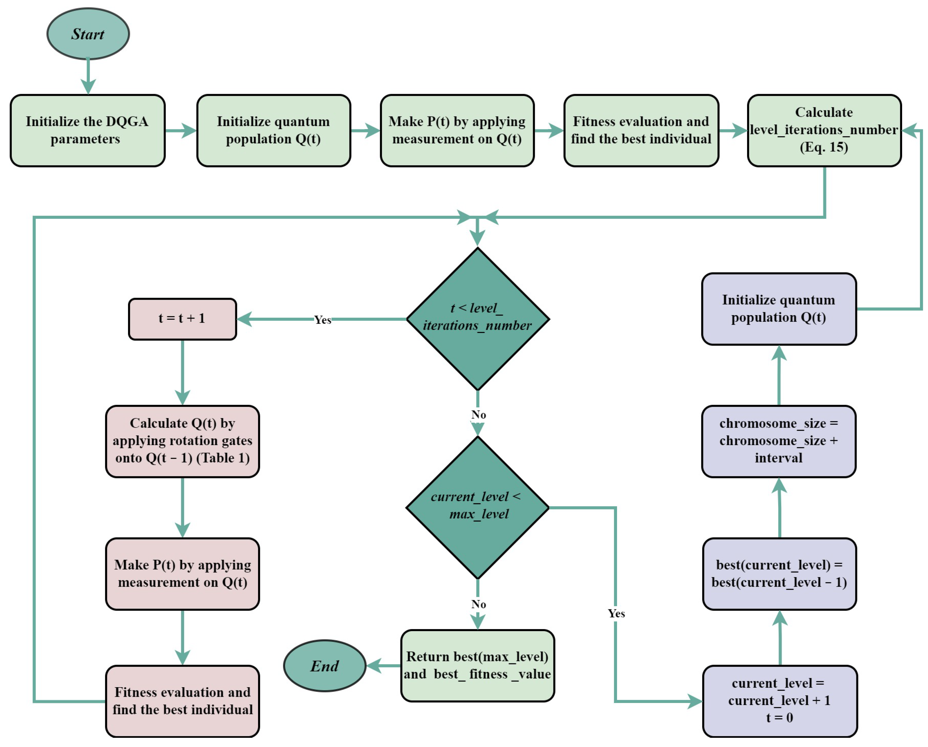
Algorithm 1 The pseudo-code of DQGA
  1:
initialize DQGA parameters ( m i n _ l e n g t h , m a x _ l e n g t h , i n t e r v a l )
  2:
c u r r e n t _ l e v e l 1
  3:
Calculate m a x _ l e v e l using Equation (8)
  4:
c h r o m o s o m e _ s i z e m i n _ l e n g t h
  5:
t 0
  6:
Initialize quantum population Q ( t )
  7:
Make binary population P ( t ) by applying measurement on Q ( t )
  8:
Evaluate fitness and find the best individual
  9:
Calculate l e v e l _ i t e r a t i o n s _ n u m b e r using Equation (16)
10:
while  ( c u r r e n t _ l e v e l m a x _ l e v e l )  do
11:
    while  ( t < l e v e l _ i t e r a t i o n s _ n u m b e r )  do
12:
         t t + 1
13:
        Calculate Q ( t ) using rotation gates on Q ( t 1 ) from Table 1
14:
        Make binary population P ( t ) by applying measurement on Q ( t )
15:
        Evaluate fitness and find the best individual
16:
    end while
17:
     t 0
18:
     c u r r e n t _ l e v e l c u r r e n t _ l e v e l + 1
19:
     b e s t _ i n d i v i d u a l ( c u r r e n t _ l e v e l ) b e s t _ i n d i v i d u a l ( c u r r e n t _ l e v e l 1 )
20:
     c h r o m o s o m e _ s i z e c h r o m o s o m e _ s i z e + i n t e r v a l
21:
    Initialize quantum population Q ( t )
22:
end while
23:
return  b e s t _ i n d i v i d u a l ( m a x _ l e v e l ) , b e s t _ f i t n e s s _ v a l u e
Table 1. Look-up table for DQGA.
x i b i f ( x ) f ( b ) Δ θ i
00falseEquation (15)
00trueEquation (15)
01falseEquation (10)
01trueEquation (12)
10falseEquation (11)
10trueEquation (13)
11falseEquation (14)
11trueEquation (14)
The main advantage of the lengthening chromosome strategy is local optima avoidance. At the early levels of the algorithm, we do not have many points on the search space, as the small number of bits cannot represent many numbers. Because of this, the chance of the local optima being found in the first levels is minuscule. This fact is also true for the global optimum, but we do not need to find the global optimum solution at the early stages. The algorithm can take its time searching all over the search space even with low precision and gradually elevate the focus at the endmost levels to exploit for the global best solution. We can be more confident that the algorithm would not become trapped in the local optima in this way.
The algorithm starts with a level of precision with chromosomes of length m i n _ l e n g t h for each dimension and increases the length of the chromosomes by i n t e r v a l genomes until the chromosomes length reaches m a x _ l e n g t h . So, the number of levels can be calculated by Equation (8).
m a x _ l e v e l = m a x _ l e n g t h m i n _ l e n g t h i n t e r v a l + 1 .

3.2. Look-Up Table with Adaptive Rotation Steps
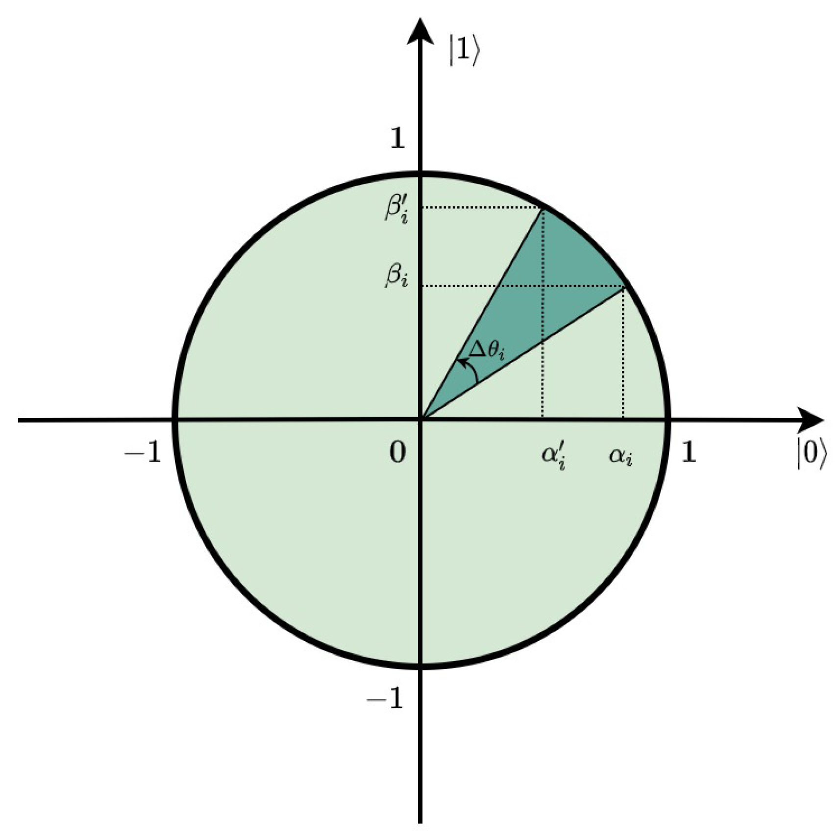
In DQGA, we introduced an adaptive look-up table to boost searchability. For the sake of simplicity and to gain better control of the quantum search space, all states are limited to reside between 0 to 90 degrees. Qubits with states closer to 90 degrees are more likely to collapse to 1 after measurement, while the probability for those closer to 0 degrees to be measured into 0 is more. We try to push the qubits to states that seem to yield better solutions during the algorithm. At early iterations of each level of the algorithm, the rotation steps toward the more fitted state are relatively small, giving the chance for the qubit to be measured even to the opposite state. The algorithm diversifies the search in this manner (exploration phase). As the number of iterations grows, the rotation steps become larger to make the qubit to be more and more likely to be measured into the best solution’s state (exploitation phase). The rotation steps are adjusted by coefficient m, which increases gradually throughout the iterations of each level, leading the rotation steps to become more prominent. Coefficient m is calculated using Equation (9).
m = 1 a b ( i t e r a t i o n / l e v e l _ i t e r a t i o n s _ n u m b e r ) , a b + 1 ,
where a and b are tuning parameters and in this paper we set them to 1.1 and 0.1, respectively.
To determine the rotation step Δ θ for each qubit, we consider three cases:
  • When the i t h bit of the best fitted binary solution of the previous generation b and current chromosome x are not equal, and b is more fitted than x , we rotate the corresponding qubit state in a direction that makes it more likely to collapse into the state of b i with a huge step. The rotation size of a huge step is formulated in Equation (10) for b i = 1 and x i = 0 and in and Equation (11) for b i = 0 and x i = 1 .
    Δ θ i = ( π / 2 θ i ) × m
    Δ θ i = θ i × m ,
    where m is the adjustment coefficient calculated by Equation (8).
  • When the i t h bit of the best fitted individual b and current chromosome x are different and x has a higher fitness value in comparison to b, the corresponding qubit is pushed to the state of x i but this time with a little caution or hesitation, as the previous iteration’s best individual guides us conversely. This leads to a relatively smaller rotation size, called medium step. Equations (12) and (13) show the mathematical representation of the case with b i = 1 and x i = 0 and the case with b i = 0 and x i = 1 , respectively.
    Δ θ i = ( π / 2 θ i ) × m 20
    Δ θ i = θ i × m 20 .
  • The last case is when b i and x i are identical. In this case, we do not care about which individual yields better fitness, as both of them share a similar state. So, we just move the qubit state by a tiny step in order to slightly confirm the last iteration’s best individual state regardless of the fitness comparison. These minor fluctuations help to keep the diversity of the population. Equation (14) expresses the tiny step when b i and x i are in state ‘1’, while Equation 15 shows otherwise.
    Δ θ i = ( π / 2 θ i ) × m 500
    Δ θ i = θ i × m 500 .
As Δ θ i is proportional to qubit’s state θ i , the rotation steps are calculated adaptively. It means that the wider the angle between the current state and the desired ket, the larger the rotation step will be. Table 1 presents the look-up table of DQGA and summarizes all the possible cases and their corresponding rotation steps.

3.3. Distribution of Generations in Different Precision Levels

As DQGA utilizes different chromosome sizes during the algorithm, we must assign a certain number of iterations to each level. Intuitively, it is clear that levels with small chromosome sizes need fewer epochs to reach a suitable solution in comparison to those consisting of a larger amount of genomes. Because when we use low levels of precision, the number of potential solutions is far less than the case with high levels of precision. As a result, we determined to distribute the whole iteration number to get consistently larger for more extended chromosome sizes. Equation (15) gives the number of iterations at each level.
l e v e l _ i t e r a t i o n s _ n u m b e r = L m a x _ l e n g t h ( m a x _ l e n g t h + 1 ) / 2 × n ,
where L is the number of each level and n is the whole number of iterations. The sum of the epochs of all levels equals to the whole number of generations. So, we have:
k = 1 m a x _ l e v e l l e v e l _ i t e r a t i o n s _ n u m b e r k = n .

4. Experimental Results and Comparison Discussion

In this section, the comparison results of utilizing the proposed algorithm to solve various optimization problems are presented to assess its efficiency and performance. The DQGA approach is applied to 10 benchmark functions and three classical constrained engineering problems. Furthermore, we applied the Wilcoxon rank-sum test in order to show the significance of the difference between the proposed algorithm and comparison algorithms’ results.

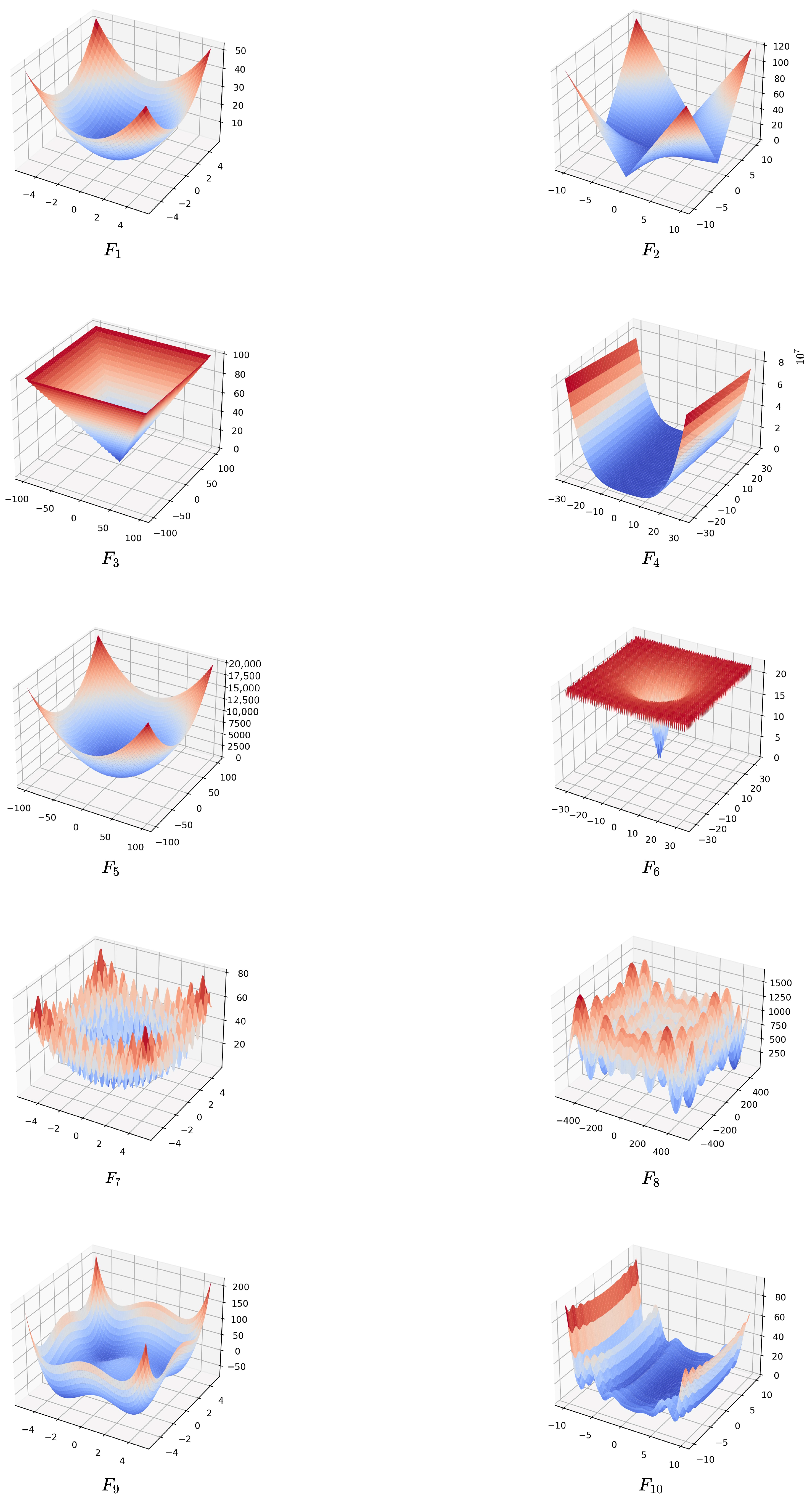
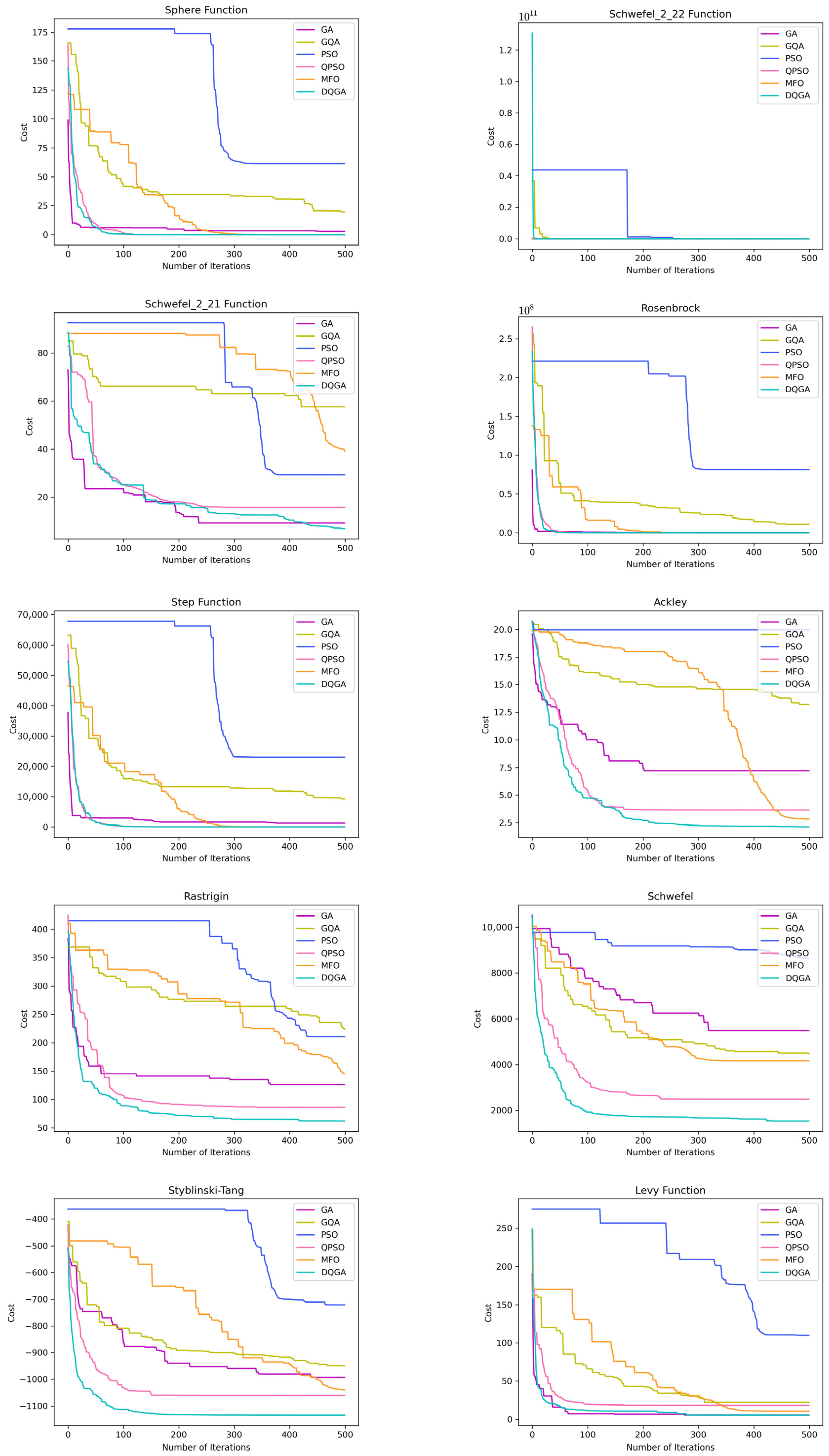
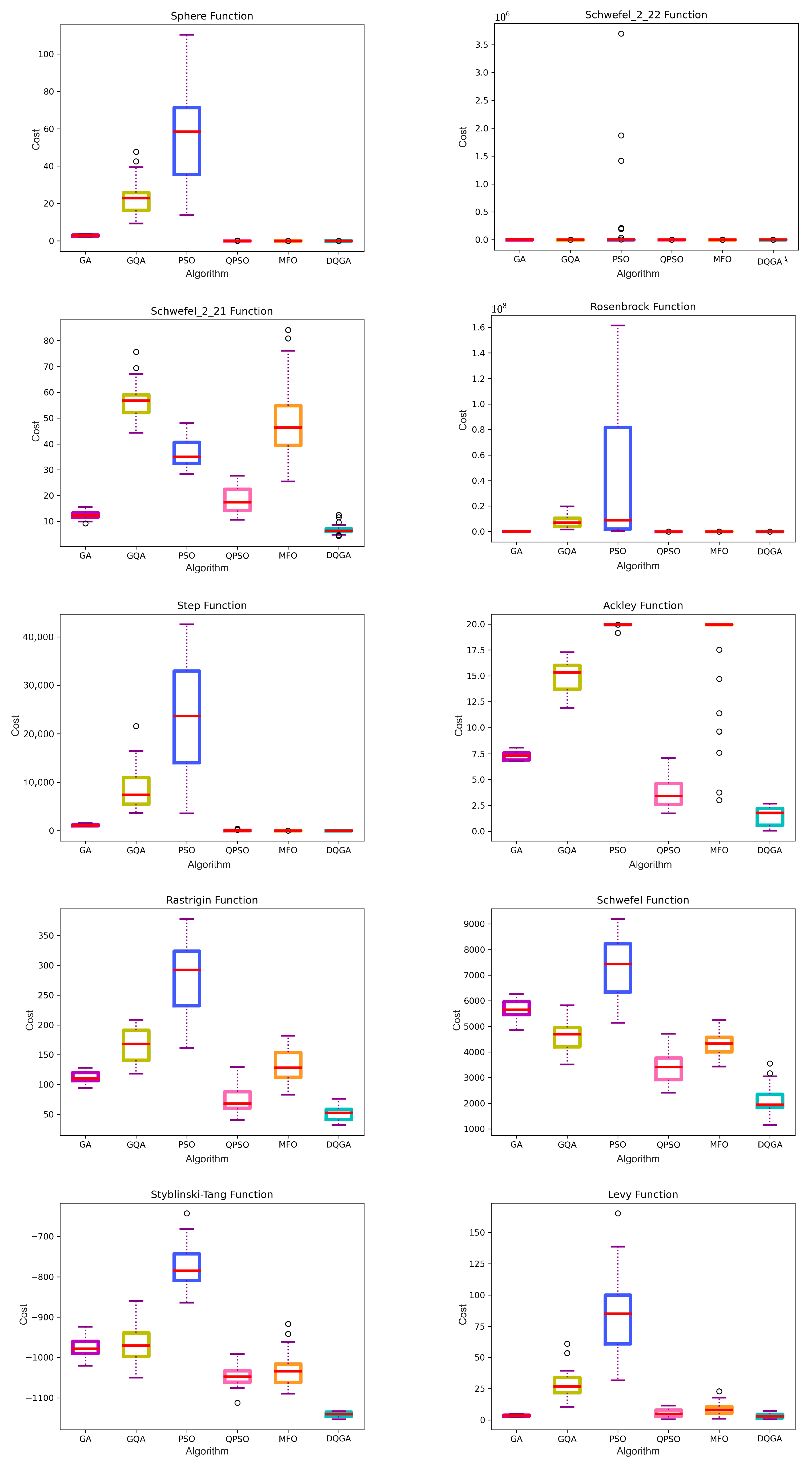
4.1. Testing DQGA on Benchmark Functions

To show the abilities of the metaheuristic algorithms, it is a common practice to test the metaheuristic algorithms by several benchmark functions with different properties. We chose 10 of the most famous benchmark functions from the optimization literature. The description, domain, and the optima of the benchmark functions are taken from [51,52,53]. The benchmark functions are depicted in Table 2 and are visualized in Figure 5. The first five functions are unimodal, meaning they have one global optimum and no local optima. Unimodal functions are suitable for testing the exploitation ability of optimization algorithms. Conversely, the last five benchmark functions are more challenging problems and are called multimodal functions. Each of these consists of numerous local optima. The number of dimensions for all the benchmark functions is set to 30.
We compared the results with five well-known and highly regarded metaheuristic algorithms, namely GA [54], GQA [8], PSO [55] which is, QPSO [56], and MFO [57]. The Python library Mealpy [58] is utilized to implement GA, PSO, and MFO algorithms for the comparison purpose. The number of iterations and the population size for all algorithms is set to 500 and 30, respectively. Table 3 shows the values of parameters for all algorithms in this experimental comparison.
As can be seen in Table 4, the results of DQGA for the benchmark functions are promising in comparison to other algorithms. For unimodal benchmark functions, the proposed algorithm yields the best average results for all the benchmark functions except for the Sphere function, which is the second best after MFO. The results for the multimodal test functions, which are more similar to real-world problems and are more challenging, are even better, and DQGA outperforms all the other algorithms in all multimodal benchmark functions.
In order to test the significance of the difference in the results, the Wilcoxon statistical test is applied pairwise between DQGA and other comparative algorithms with the level of significance α = 0.05 . The p-values obtained from the test are given in Table 5. From the results, it is apparent that none of the p-values is greater than 0.05, rejecting the null hypothesis and confirming the significance of the results.
To test the time efficiency of the proposed algorithm, we provided convergence curves that show and compare the algorithms’ iterations needed to reach specific fitness values. It should be noted that comparing the number of iterations is a more fair criterion than the total execution time, especially in our case, as the algorithms are of different implementation approaches that might have a substantial impact on the total execution time. For instance, multi-processing and multi-threading approaches can reduce the computational time to nearly one-fourth on a four-core CPU. For this reason, we chose to compare the algorithms based on the number of iterations criterion rather than the total execution time.
Figure 6 presents the convergence behavior of different algorithms in this experiment. The convergence curve of the proposed algorithm shows a steady improvement in the solution as the generations pass. The convergence speed is also very competitive with other algorithms. The pace is faster than other algorithms in most cases except for the Sphere function, Schwefel 2.21, Rosenbrock function, and Levy function which was roughly equivalent to GA and QPSO algorithms.
Boxplots in Figure 7 show the range of solutions in different runs. The low range of distribution of results for DQGA compared to the other algorithms verifies the reliability and consistency of the algorithm. The ranges are relatively lower or at least comparable to the best for DQGA except for the Levy function, in which the GA yielded more consistent results.

4.2. Constrained Engineering Design Optimization Using DQGA

As the ultimate purpose of metaheuristics is to tackle complex real-world problems and not merely solve mathematical benchmark functions, we also applied DQGA to three classical constrained engineering problems. The engineering problems are the pressure vessel design problem, the speed reducer design problem, and the cantilever beam design problem. The constraint handling technique used in this paper is the death penalty, meaning that the constraint violation leads to a substantial negative fitness and inability to compete with other solutions. The results obtained by DQGA were utterly satisfying and are presented in the following subsections in detail.

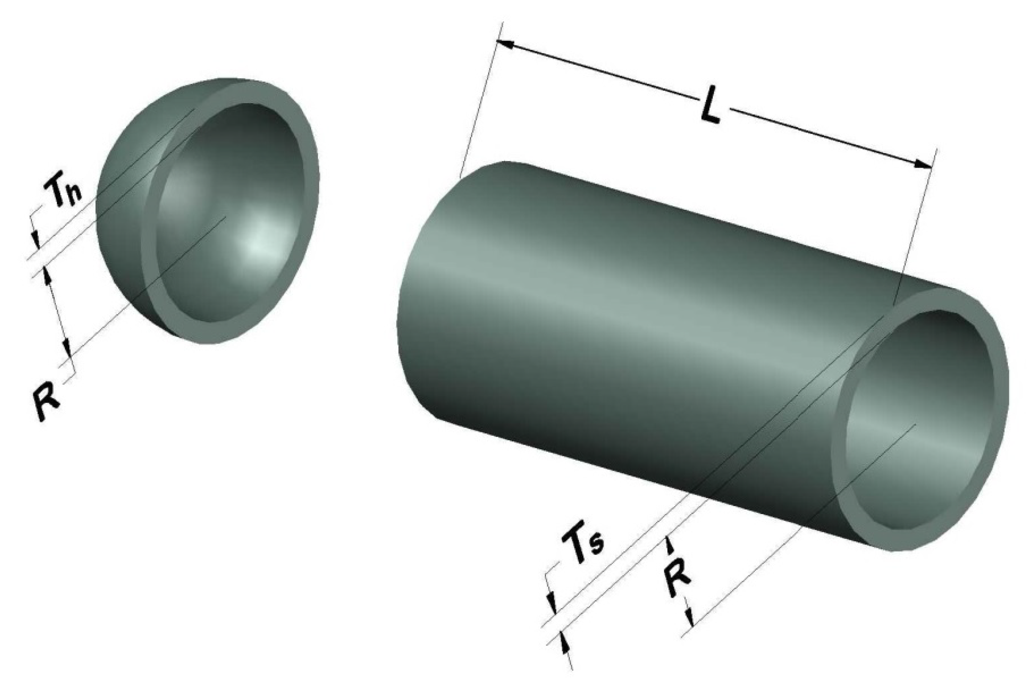
4.2.1. Pressure Vessel Design

The pressure vessel design problem was first introduced by [59]. The problem objective is to minimize the material, forming, and welding costs of producing a cylindrical vessel with two hemispherical caps at both ends (see Figure 8). The problem consists of four design variables: thickness of shell T S , thickness of head T h , inner radius R, and the cylindrical section’s length L. The problem is formulated as follows:
C o n s i d e r x = [ x 1 x 2 x 3 x 4 ] = [ T s T h R L ] , M i n i m i z e f ( x ) = 0.6224 x 1 x 3 x 4 + 1.7781 x 2 x 3 2 + 3.1661 x 1 2 x 4 + 19.84 x 1 2 x 3 , S u b j e c t t o g 1 ( x ) = 0.0193 x 3 x 1 0 , g 2 ( x ) = 0.00954 x 3 x 2 0 , g 3 ( x ) = 1296000 π x 3 2 x 4 4 3 π x 3 3 0 , D o m a i n 0 x 1 , x 2 99 , 10 x 3 , x 4 200 .
The results of applying DQGA to the pressure vessel design problem are given in Table 6 and are compared with the reported results of Branch-bound [60], GA [54], GWO [61], WOA [62], HHO [63], WSA [64], and AOA [65] algorithms. The results confirm that DQGA outperformed the other algorithms in solving this problem.

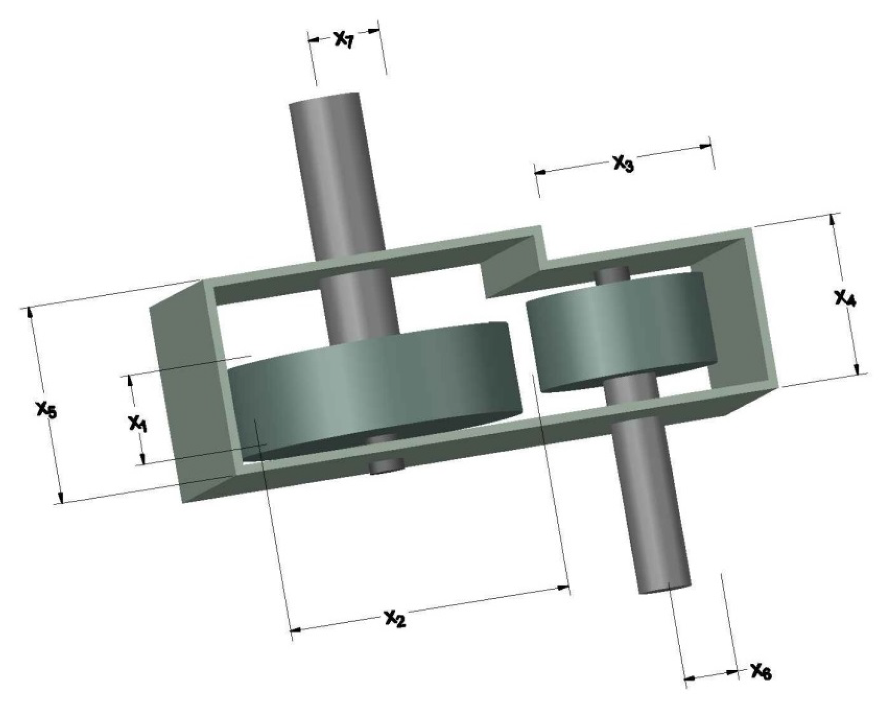
4.2.2. Speed Reducer Design

The speed reducer design problem aims to minimize the total weight of a speed reducer by concerning the bending stress on the gear teeth, stress on the surface, transverse deflections, and stresses in shafts constraints [67]. The problem has six continuous variables and one discrete variable x 3 , which corresponds to the number of teeth on the pinion. The structure of a speed reducer is given in Figure 9, and the problem description is defined in the following:
C o n s i d e r x = [ x 1 x 2 x 3 x 4 x 5 x 6 x 7 ] , M i n i m i z e f ( x ) = 0.7854 x 1 x 2 2 ( 3.3333 x 3 2 + 14.9334 x 3 43.0934 ) 1.508 x 1 ( x 6 2 + x 7 2 ) + 7.4777 ( x 6 3 + x 7 3 ) + 0.7854 ( x 4 x 6 2 + x 5 x 7 2 ) , S u b j e c t t o g 1 ( x ) = 27 x 1 x 2 2 x 3 1 0 , g 2 ( x ) = 397.5 x 1 x 2 2 x 3 2 1 0 , g 3 ( x ) = 1.93 x 4 3 x 2 x 3 x 6 4 1 0 , g 4 ( x ) = 1.93 x 5 3 x 2 x 3 x 7 4 1 0 , g 5 ( x ) = ( 745 x 4 / x 2 x 3 ) 2 + 16.9 × 10 6 110 x 6 3 1 0 , g 6 ( x ) = ( 745 x 4 / x 2 x 3 ) 2 + 157.5 × 10 6 85 x 7 3 1 0 , g 7 ( x ) = x 2 x 3 40 1 0 , g 8 ( x ) = 5 x 2 x 1 1 0 , g 9 ( x ) = x 1 12 x 2 1 0 , g 10 ( x ) = 1.5 x 6 + 1.9 x 4 1 0 , g 11 ( x ) = 1.1 x 7 + 1.9 x 5 1 0 , D o m a i n 2.6 x 1 3.6 , 0.7 x 2 0.8 , 17 x 3 28 , 7.3 x 4 8.3 , 7.8 x 5 8.3 , 2.9 x 6 3.9 , 5.0 x 7 5.3
Table 7 presents the comparison results for solving the speed reducer design problem by the proposed algorithm and CS [68], FA [69], WSA [64], hHHO-SCA [70], AAO [71], AO [72], and AOA [65] algorithms. It can be seen that DQGA obtained the best result among the comparison algorithms.

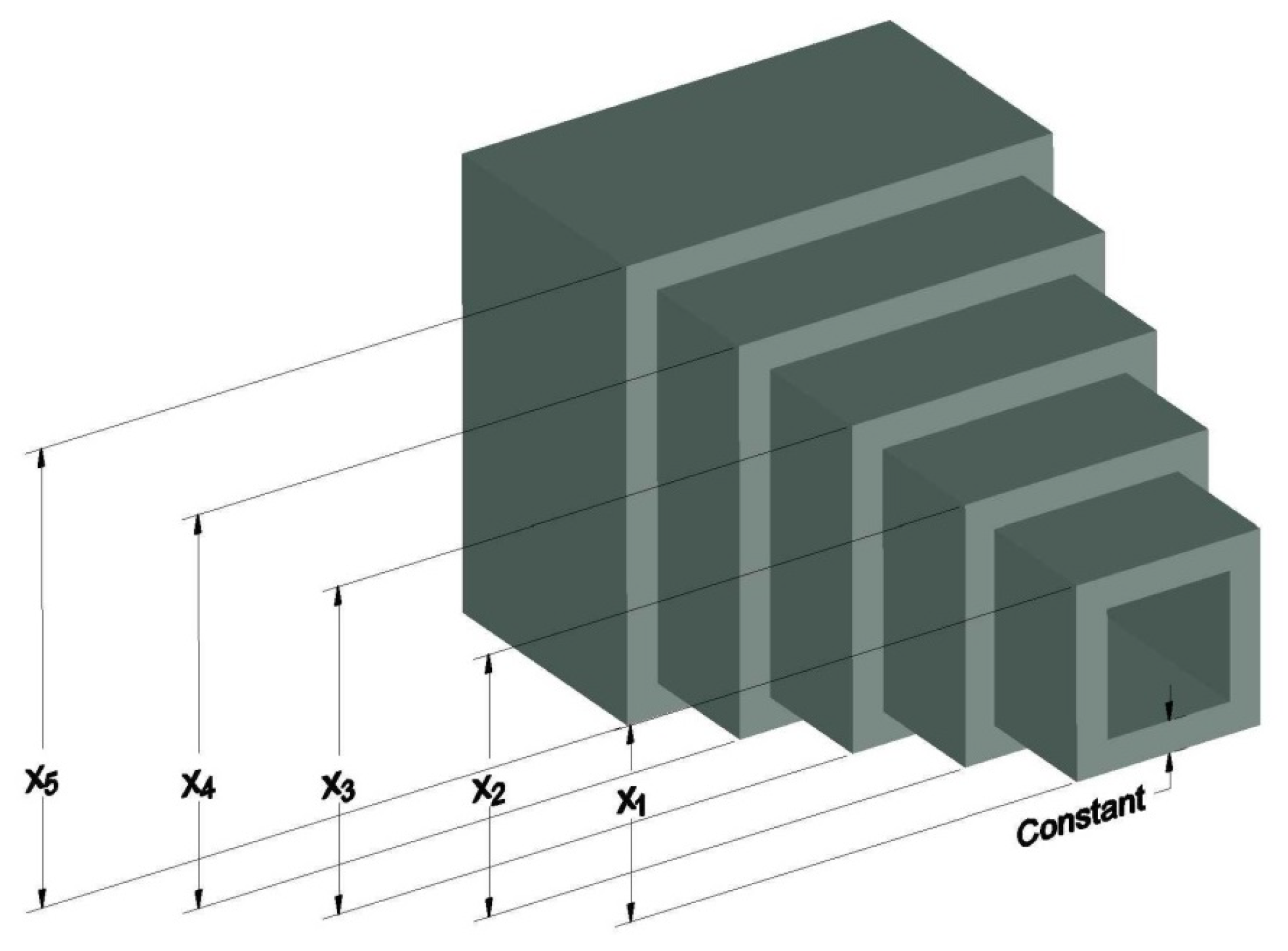
4.2.3. Cantilever Beam Design

The purpose of the problem is to find the minimum weight for a cantilever beam containing five hollow square based elements with constant thickness (Figure 10). The beam is fixed at the larger end with a vertical force acting at the other end.
C o n s i d e r x = [ x 1 x 2 x 3 x 4 x 5 ] , M i n i m i z e f ( x ) = 0.6224 ( x 1 + x 2 + x 3 + x 4 + x 5 ) , S u b j e c t t o g ( x ) = 61 x 1 3 + 27 x 2 3 + 19 x 3 3 + 7 x 4 3 + 1 x 5 3 1 0 , D o m a i n 0.01 x 1 , x 2 , x 3 , x 4 , x 5 100 .
DQGA is applied to this problem and the results are compared with several algorithms including CS [68], SOS [73], MFO [57], GCA_I [74], GCA_II [74], SMA [75], and AO [72]. The results are given in Table 8. From the results, it can be seen that DQGA presents the optimal solution for this problem in comparison to the other algorithms.

5. Conclusions and Potential Future Work

In this paper, we proposed a modified QGA called DQGA, which focuses not only on exploration and exploitation abilities but on smoothing the transition between the mentioned phases. These improvements are achieved by an adaptive look-up table and a lengthening chromosomes strategy, which clarifies the search space gradually and postpones the convergence to high precision solutions to the ending generations, avoiding the algorithm from premature convergence and being trapped in the local optima. Experimental tests were conducted to ensure that the proposed concepts are effective in practice. DQGA outperformed the comparative algorithms in most cases, especially for multimodal benchmark functions and the more challenging engineering design problems.
These promising results give hope that the presented algorithm has the potential to tackle other real-world optimization problems. Future studies may include applying DQGA to various applications, such as network applications, fuzzy controller design, image thresholding, flight control, and structural design. In addition, the binary-coded nature of the proposed algorithm makes it suitable for discrete optimization problems like the travelling salesman problem, the 01 knapsack problem, the job-scheduling problem, airport gate allocation, and feature selection. Moreover, a systematic and adaptive tuning of parameters of DQGA, such as the minimum and the maximum length of chromosomes and incremental intervals, can be considered for further studies.

Author Contributions

S.H. under the supervision of M.H. and S.A.H. developed and implemented the main idea and wrote the initial draft of the manuscript. S.H., M.H., S.A.H. and X.Z. verified the idea and the results and revised the manuscript. All authors have read and agreed to the published version of the manuscript.

Funding

This research received no external funding.

Institutional Review Board Statement

Not applicable.

Data Availability Statement

Data are available on request.

Conflicts of Interest

The authors declare no conflict of interest.

References

  1. Hemanth, J.; Balas, V. Nature Inspired Optimization Techniques for Image Processing Applications; Springer: Berlin/Heidelberg, Germany, 2019; Volume 150. [Google Scholar]
  2. Gandomi, A.; Yang, X.; Talatahari, S.; Alavi, A. Metaheuristic Applications in Structures and Infrastructures; Elsevier: Amsterdam, The Netherlands, 2013. [Google Scholar]
  3. Elshaer, R.; Awad, H. A taxonomic review of metaheuristic algorithms for solving the vehicle routing problem and its variants. Comput. Ind. Eng. 2020, 140, 106242. [Google Scholar] [CrossRef]
  4. Agrawal, P.; Abutarboush, H.; Ganesh, T.; Mohamed, A. Metaheuristic algorithms on feature selection: A survey of one decade of research (2009–2019). IEEE Access 2021, 9, 26766–26791. [Google Scholar] [CrossRef]
  5. Doering, J.; Kizys, R.; Juan, A.; Fito, A.; Polat, O. Metaheuristics for rich portfolio optimisation and risk management: Current state and future trends. Oper. Res. Perspect. 2019, 6, 100121. [Google Scholar] [CrossRef]
  6. Calvet, L.; Benito, S.; Juan, A.; Prados, F. On the role of metaheuristic optimization in bioinformatics. Int. Trans. Oper. Res. 2023, 30, 2909–2944. [Google Scholar] [CrossRef]
  7. Bhavya, R.; Elango, L. Ant-Inspired Metaheuristic Algorithms for Combinatorial Optimization Problems in Water Resources Management. Water 2023, 15, 1712. [Google Scholar] [CrossRef]
  8. Han, K.H.; Kim, J.H. Genetic quantum algorithm and its application to combinatorial optimization problem. In Proceedings of the 2000 Congress on Evolutionary Computation, CEC00 (Cat. No. 00TH8512), La Jolla, CA, USA, 16–19 July 2000; Volume 2, pp. 1354–1360. [Google Scholar]
  9. Han, K.H.; Kim, J.H. Quantum-inspired evolutionary algorithm for a class of combinatorial optimization. IEEE Trans. Evol. Comput. 2002, 6, 580–593. [Google Scholar] [CrossRef]
  10. Si-Jung, R.; Jun-Seuk, G.; Seung-Hwan, B.; Songcheol, H.; Jong-Hwan, K. Feature-based hand gesture recognition using an FMCW radar and its temporal feature analysis. IEEE Sens. J. 2018, 18, 7593–7602. [Google Scholar]
  11. Dey, A.; Dey, S.; Bhattacharyya, S.; Platos, J.; Snasel, V. Novel quantum inspired approaches for automatic clustering of gray level images using particle swarm optimization, spider monkey optimization and ageist spider monkey optimization algorithms. Appl. Soft Comput. 2020, 88, 106040. [Google Scholar] [CrossRef]
  12. Choudhury, A.; Samanta, S.; Pratihar, S.; Bandyopadhyay, O. Multilevel segmentation of Hippocampus images using global steered quantum inspired firefly algorithm. Appl. Intell. 2021, 52, 7339–7372. [Google Scholar] [CrossRef]
  13. Kaveh, A.; Dadras, A.; Geran malek, N. Robust design optimization of laminated plates under uncertain bounded buckling loads. Struct. Multidiscip. Optim. 2019, 59, 877–891. [Google Scholar] [CrossRef]
  14. Arzani, H.; Kaveh, A.; Kamalinejad, M. Optimal design of pitched roof rigid frames with non-prismatic members using quantum evolutionary algorithm. Period. Polytech. Civ. Eng. 2019, 63, 593–607. [Google Scholar] [CrossRef]
  15. Zhang, S.; Zhou, G.; Zhou, Y.; Luo, Q. Quantum-inspired satin bowerbird algorithm with Bloch spherical search for constrained structural optimization. J. Ind. Manag. Optim. 2021, 17, 3509. [Google Scholar] [CrossRef]
  16. Talatahari, S.; Azizi, M.; Toloo, M.; Baghalzadeh Shishehgarkhaneh, M. Optimization of Large-Scale Frame Structures Using Fuzzy Adaptive Quantum Inspired Charged System Search. Int. J. Steel Struct. 2022, 22, 686–707. [Google Scholar] [CrossRef]
  17. Konar, D.; Bhattacharyya, S.; Sharma, K.; Sharma, S.; Pradhan, S.R. An improved hybrid quantum-inspired genetic algorithm (HQIGA) for scheduling of real-time task in multiprocessor system. Appl. Soft Comput. 2017, 53, 296–307. [Google Scholar] [CrossRef]
  18. Alam, T.; Raza, Z. Quantum genetic algorithm based scheduler for batch of precedence constrained jobs on heterogeneous computing systems. J. Syst. Softw. 2018, 135, 126–142. [Google Scholar] [CrossRef]
  19. Saad, H.M.; Chakrabortty, R.K.; Elsayed, S.; Ryan, M.J. Quantum-inspired genetic algorithm for resource-constrained project-scheduling. IEEE Access 2021, 9, 38488–38502. [Google Scholar] [CrossRef]
  20. Wu, X.; Wu, S. An elitist quantum-inspired evolutionary algorithm for the flexible job-shop scheduling problem. J. Intell. Manuf. 2017, 28, 1441–1457. [Google Scholar] [CrossRef]
  21. Singh, K.V.; Raza, Z. A quantum-inspired binary gravitational search algorithm–based job-scheduling model for mobile computational grid. Concurr. Comput. Pract. Exp. 2017, 29, e4103. [Google Scholar] [CrossRef]
  22. Liu, M.; Yi, S.; Wen, P. Quantum-inspired hybrid algorithm for integrated process planning and scheduling. Proc. Inst. Mech. Eng. Part B J. Eng. Manuf. 2018, 232, 1105–1122. [Google Scholar] [CrossRef]
  23. Gupta, S.; Mittal, S.; Gupta, T.; Singhal, I.; Khatri, B.; Gupta, A.K.; Kumar, N. Parallel quantum-inspired evolutionary algorithms for community detection in social networks. Appl. Soft Comput. 2017, 61, 331–353. [Google Scholar] [CrossRef]
  24. Qu, Z.; Li, T.; Tan, X.; Li, P.; Liu, X. A modified quantum-inspired evolutionary algorithm for minimising network coding operations. Int. J. Wirel. Mob. Comput. 2020, 19, 401–410. [Google Scholar] [CrossRef]
  25. Li, F.; Liu, M.; Xu, G. A quantum ant colony multi-objective routing algorithm in WSN and its application in a manufacturing environment. Sensors 2019, 19, 3334. [Google Scholar] [CrossRef]
  26. Mirhosseini, M.; Fazlali, M.; Malazi, H.T.; Izadi, S.K.; Nezamabadi-pour, H. Parallel Quadri-valent Quantum-Inspired Gravitational Search Algorithm on a heterogeneous platform for wireless sensor networks. Comput. Electr. Eng. 2021, 92, 107085. [Google Scholar] [CrossRef]
  27. Chou, Y.H.; Kuo, S.Y.; Jiang, Y.C.; Wu, C.H.; Shen, J.Y.; Hua, C.Y.; Huang, P.S.; Lai, Y.T.; Tong, Y.F.; Chang, M.H. A novel quantum-inspired evolutionary computation-based quantum circuit synthesis for various universal gate libraries. In Proceedings of the Genetic and Evolutionary Computation Conference Companion 2022, Boston, MA, USA, 9–13 July 2022; pp. 2182–2189. [Google Scholar]
  28. Ramos, A.C.; Vellasco, M. Chaotic quantum-inspired evolutionary algorithm: Enhancing feature selection in BCI. In Proceedings of the 2020 IEEE Congress on Evolutionary Computation (CEC), Glasgow, UK, 19–24 July 2020; pp. 1–8. [Google Scholar]
  29. Barani, F.; Mirhosseini, M.; Nezamabadi-Pour, H. Application of binary quantum-inspired gravitational search algorithm in feature subset selection. Appl. Intell. 2017, 47, 304–318. [Google Scholar] [CrossRef]
  30. Di Martino, F.; Sessa, S. A novel quantum inspired genetic algorithm to initialize cluster centers in fuzzy C-means. Expert Syst. Appl. 2022, 191, 116340. [Google Scholar] [CrossRef]
  31. Chou, Y.H.; Lai, Y.T.; Jiang, Y.C.; Kuo, S.Y. Using Trend Ratio and GNQTS to Assess Portfolio Performance in the US Stock Market. IEEE Access 2021, 9, 88348–88363. [Google Scholar] [CrossRef]
  32. Qi, B.; Nener, B.; Xinmin, W. A quantum inspired genetic algorithm for multimodal optimization of wind disturbance alleviation flight control system. Chin. J. Aeronaut. 2019, 32, 2480–2488. [Google Scholar]
  33. Yi, J.H.; Lu, M.; Zhao, X.J. Quantum inspired monarch butterfly optimisation for UCAV path planning navigation problem. Int. J. Bio-Inspired Comput. 2020, 15, 75–89. [Google Scholar] [CrossRef]
  34. Dahi, Z.A.E.M.; Mezioud, C.; Draa, A. A quantum-inspired genetic algorithm for solving the antenna positioning problem. Swarm Evol. Comput. 2016, 31, 24–63. [Google Scholar] [CrossRef]
  35. Cai, X.; Zhao, H.; Shang, S.; Zhou, Y.; Deng, W.; Chen, H.; Deng, W. An improved quantum-inspired cooperative co-evolution algorithm with muli-strategy and its application. Expert Syst. Appl. 2021, 171, 114629. [Google Scholar] [CrossRef]
  36. Sadeghi Hesar, A.; Kamel, S.R.; Houshmand, M. A quantum multi-objective optimization algorithm based on harmony search method. Soft Comput. 2021, 25, 9427–9439. [Google Scholar] [CrossRef]
  37. Ross, O.H.M. A review of quantum-inspired metaheuristics: Going from classical computers to real quantum computers. IEEE Access 2019, 8, 814–838. [Google Scholar] [CrossRef]
  38. Hakemi, S.; Houshmand, M.; KheirKhah, E.; Hosseini, S.A. A review of recent advances in quantum-inspired metaheuristics. Evol. Intell. 2022, 1–16. [Google Scholar]
  39. Holland, J.H. Genetic algorithms. Sci. Am. 1992, 267, 66–73. [Google Scholar] [CrossRef]
  40. Houshmand, M.; Mohammadi, Z.; Zomorodi-Moghadam, M.; Houshmand, M. An evolutionary approach to optimizing teleportation cost in distributed quantum computation. Int. J. Theor. Phys. 2020, 59, 1315–1329. [Google Scholar] [CrossRef]
  41. Daei, O.; Navi, K.; Zomorodi-Moghadam, M. Optimized quantum circuit partitioning. Int. J. Theor. Phys. 2020, 59, 3804–3820. [Google Scholar] [CrossRef]
  42. Ghodsollahee, I.; Davarzani, Z.; Zomorodi, M.; Pławiak, P.; Houshmand, M.; Houshmand, M. Connectivity matrix model of quantum circuits and its application to distributed quantum circuit optimization. Quantum Inf. Process. 2021, 20, 1–21. [Google Scholar] [CrossRef]
  43. Dadkhah, D.; Zomorodi, M.; Hosseini, S.E. A new approach for optimization of distributed quantum circuits. Int. J. Theor. Phys. 2021, 60, 3271–3285. [Google Scholar] [CrossRef]
  44. Lukac, M.; Perkowski, M. Evolving quantum circuits using genetic algorithm. In Proceedings of the 2002 NASA/DoD Conference on Evolvable Hardware, Alexandria, VA, USA, 15–18 July 2002; pp. 177–185. [Google Scholar]
  45. Mukherjee, D.; Chakrabarti, A.; Bhattacherjee, D. Synthesis of quantum circuits using genetic algorithm. Int. J. Recent Trends Eng. 2009, 2, 212. [Google Scholar]
  46. Sünkel, L.; Martyniuk, D.; Mattern, D.; Jung, J.; Paschke, A. GA4QCO: Genetic algorithm for quantum circuit optimization. arXiv 2023, arXiv:2302.01303. [Google Scholar]
  47. Houshmand, M.; Saheb Zamani, M.; Sedighi, M.; Houshmand, M. GA-based approach to find the stabilizers of a given sub-space. Genet. Program. Evolvable Mach. 2015, 16, 57–71. [Google Scholar] [CrossRef]
  48. Kim, I.Y.; De Weck, O. Variable chromosome length genetic algorithm for progressive refinement in topology optimization. Struct. Multidiscip. Optim. 2005, 29, 445–456. [Google Scholar] [CrossRef]
  49. Pawar, S.N.; Bichkar, R.S. Genetic algorithm with variable length chromosomes for network intrusion detection. Int. J. Autom. Comput. 2015, 12, 337–342. [Google Scholar] [CrossRef]
  50. Sadeghi Hesar, A.; Houshmand, M. A memetic quantum-inspired genetic algorithm based on tabu search. Evol. Intell. 2023, 1–17. [Google Scholar]
  51. Yao, X.; Liu, Y.; Lin, G. Evolutionary programming made faster. IEEE Trans. Evol. Comput. 1999, 3, 82–102. [Google Scholar]
  52. Molga, M.; Smutnicki, C. Test functions for optimization needs. Test Funct. Optim. Needs 2005, 101, 48. [Google Scholar]
  53. Jamil, M.; Yang, X.S. A literature survey of benchmark functions for global optimization problems. arXiv 2013, arXiv:1308.4008. [Google Scholar]
  54. Holland, J.H. Adaptation in Natural and Artificial Systems: An Introductory Analysis with Applications to Biology, Control, and Artificial Intelligence; MIT Press: Cambridge, UK, 1992. [Google Scholar]
  55. Sun, J.; Feng, B.; Xu, W. Particle swarm optimization with particles having quantum behavior. In Proceedings of the 2004 Congress on Evolutionary Computation (IEEE Cat. No. 04TH8753), Portland, OR, USA, 19–23 June 2004; Volume 1, pp. 325–331. [Google Scholar]
  56. Yang, S.; Wang, M.; Jiao, L. A quantum particle swarm optimization. In Proceedings of the 2004 Congress on Evolutionary Computation (IEEE Cat. No. 04TH8753), Portland, OR, USA, 19–23 June 2004; Volume 1, pp. 320–324. [Google Scholar]
  57. Mirjalili, S. Moth-flame optimization algorithm: A novel nature-inspired heuristic paradigm. Knowl.-Based Syst. 2015, 89, 228–249. [Google Scholar]
  58. Van Thieu, N.; Mirjalili, S. MEALPY: An open-source library for latest meta-heuristic algorithms in Python. J. Syst. Archit. 2023, 139, 102871. [Google Scholar]
  59. Kannan, B.; Kramer, S.N. An augmented Lagrange multiplier based method for mixed integer discrete continuous optimization and its applications to mechanical design. J. Mech. Des. 1994, 116, 405–411. [Google Scholar] [CrossRef]
  60. Sandgren, E. Nonlinear Integer and Discrete Programming in Mechanical Design Optimization. J. Mech. Des. 1990, 112, 223–229. [Google Scholar] [CrossRef]
  61. Mirjalili, S.; Mirjalili, S.M.; Lewis, A. Grey wolf optimizer. Adv. Eng. Softw. 2014, 69, 46–61. [Google Scholar]
  62. Mirjalili, S.; Lewis, A. The whale optimization algorithm. Adv. Eng. Softw. 2016, 95, 51–67. [Google Scholar]
  63. Heidari, A.A.; Mirjalili, S.; Faris, H.; Aljarah, I.; Mafarja, M.; Chen, H. Harris hawks optimization: Algorithm and applications. Future Gener. Comput. Syst. 2019, 97, 849–872. [Google Scholar]
  64. Baykasoğlu, A.; Akpinar, Ş. Weighted Superposition Attraction (WSA): A swarm intelligence algorithm for optimization problems—Part 2: Constrained optimization. Appl. Soft Comput. 2015, 37, 396–415. [Google Scholar]
  65. Abualigah, L.; Diabat, A.; Mirjalili, S.; Abd Elaziz, M.; Gandomi, A.H. The arithmetic optimization algorithm. Comput. Methods Appl. Mech. Eng. 2021, 376, 113609. [Google Scholar]
  66. Coello, C.A.C. Use of a self-adaptive penalty approach for engineering optimization problems. Comput. Ind. 2000, 41, 113–127. [Google Scholar]
  67. Siddall, J.N. Analytical Decision-Making in Engineering Design; Prentice Hall: Hoboken, NJ, USA, 1972. [Google Scholar]
  68. Gandomi, A.H.; Yang, X.S.; Alavi, A.H. Cuckoo search algorithm: A metaheuristic approach to solve structural optimization problems. Eng. Comput. 2013, 29, 17–35. [Google Scholar]
  69. Baykasoğlu, A.; Ozsoydan, F.B. Adaptive firefly algorithm with chaos for mechanical design optimization problems. Appl. Soft Comput. 2015, 36, 152–164. [Google Scholar]
  70. Kamboj, V.K.; Nandi, A.; Bhadoria, A.; Sehgal, S. An intensify Harris Hawks optimizer for numerical and engineering optimization problems. Appl. Soft Comput. 2020, 89, 106018. [Google Scholar]
  71. Czerniak, J.M.; Zarzycki, H.; Ewald, D. AAO as a new strategy in modeling and simulation of constructional problems optimization. Simul. Model. Pract. Theory 2017, 76, 22–33. [Google Scholar]
  72. Abualigah, L.; Yousri, D.; Abd Elaziz, M.; Ewees, A.A.; Al-Qaness, M.A.; Gandomi, A.H. Aquila optimizer: A novel meta-heuristic optimization algorithm. Comput. Ind. Eng. 2021, 157, 107250. [Google Scholar]
  73. Cheng, M.Y.; Prayogo, D. Symbiotic organisms search: A new metaheuristic optimization algorithm. Comput. Struct. 2014, 139, 98–112. [Google Scholar]
  74. Chickermane, H.; Gea, H.C. Structural optimization using a new local approximation method. Int. J. Numer. Methods Eng. 1996, 39, 829–846. [Google Scholar]
  75. Zhao, J.; Gao, Z.M.; Sun, W. The improved slime mould algorithm with Levy flight. J. Phys. Conf. Ser. 2020, 1617, 012033. [Google Scholar] [CrossRef]
Figure 1. Updating a qubit state using quantum rotation gate.
Axioms 12 00978 g001
Figure 2. Flowchart of DQGA.
Axioms 12 00978 g002
Figure 3. An example of lengthening chromosomes.
Axioms 12 00978 g003
Figure 4. Exponential growth of precision by increasing the chromosome size. Possible points to represent different chromosome sizes for each dimension are shown.
Axioms 12 00978 g004
Figure 5. Two-dimensional representation of the benchmark functions’ search spaces.
Axioms 12 00978 g005
Figure 6. Comparison of convergence curves of DQGA and other algorithms.
Axioms 12 00978 g006
Figure 7. Box plots of the algorithms used in the comparison.
Axioms 12 00978 g007
Figure 8. Pressure vessel design problem.
Axioms 12 00978 g008
Figure 9. Speed reducer design problem.
Axioms 12 00978 g009
Figure 10. Cantilever beam design problem.
Axioms 12 00978 g010
Table 2. Description of benchmark functions.
Function NameFunction DescriptionDomain F min
Sphere Function F 1 ( x ) = i = 1 n x i 2 [ 5.12 , 5.12 ] 0
Schwefel 2.22 F 2 ( x ) = i = 1 n | x i | + i = 1 n | x i | [ 10 , 10 ] 0
Schwefel 2.21 F 3 ( x ) = max i | x i | , 1 i n [ 1.28 , 1.28 ] 0
Rosenbrock F 4 ( x ) = i = 1 n 1 100 x i + 1 x i 2 2 + ( x i 1 ) 2 [ 30 , 30 ] 0
Step Function F 5 ( x ) = i = 1 n ( x i + 0.5 ) 2 [ 100 , 100 ] 0
Ackley F 6 ( x ) = 20 exp ( 0.2 1 n i = 1 n x i 2 )
exp ( 1 n i = 1 n cos 2 π x i ) + 20 + e
[ 32 , 32 ] 0
Rastrigin F 7 ( x ) = 10 n + i = 1 n x i 2 10 cos ( 2 π x i ) [ 5.12 , 5.12 ] 0
Schwefel F 8 ( x ) = 418.9829 n i = 1 n x i sin | x i | [ 500 , 500 ] 0
Styblisky–Tang F 9 ( x ) = 1 2 i = 1 n ( x i 4 16 x i 2 + 5 x i ) [ 5 , 5 ] 39.16599 n
Levy F 10 ( x ) = sin 2 ( π ω 1 ) + i = 1 n 1 ( ω i 1 ) 2 ×
1 + 10 sin 2 ( π ω i + 1 ) +
( ω n 1 ) 2 1 + sin 2 ( 2 π ω n ) ,
w h e r e ω i = 1 + x i 1 4 , f o r i = 1 , , n
[ 10 , 10 ] 0
Table 3. Parameter values for optimization algorithms.
AlgorithmParameterValue
GA [54]Implementation typeReal-coded
Selection methodRoulette wheel
Crossover probability 80 %
Mutation methodFlip
Mutation probability 0.05 %
GQA [8]No Parameter setting
PSO [55] c 1 2
c 2 2
weight_min0.1
weight_max0.9
QPSO [56] a 1 1
a 2 0.5
MFO [57]a [ 2 , 1 ]
b1
DQGAmin_length16
max_length32
interval4
a1.1
b0.1
Table 4. Comparison results for the benchmark functions.
F GA [54]GQA [8]PSO [55]QPSO [56]MFO [57]DQGA
F 1 Mean
STD
2.90 × 10 0
4.06 × 10 1
2.32 × 10 1
9.40 × 10 0
5.58 × 10 1
2.76 × 10 1
2.39 × 10 2
3.38 × 10 2
1 . 28 × 10 5
2.53 × 10 5
3.05 × 10 4
2.02 × 10 4
F 2 Mean
STD
1.17 × 10 1
1.03 × 10 0
3.34 × 10 1
1.01 × 10 1
2.48 × 10 5
7.75 × 10 5
3.95 × 10 0
5.46 × 10 0
4.35 × 10 0
9.71 × 10 0
7 . 41 × 10 2
2.44 × 10 2
F 3 Mean
STD
1.24 × 10 1
1.30 × 10 0
5.70 × 10 1
6.53 × 10 0
3.65 × 10 1
5.26 × 10 0
1.67 × 10 1
5.07 × 10 0
4.94 × 10 1
1.41 × 10 1
7 . 86 × 10 0
2.43 × 10 0
F 4 Mean
STD
1.93 × 10 5
6.31 × 10 4
8.17 × 10 6
5.17 × 10 6
4.04 × 10 7
4.50 × 10 7
7.93 × 10 2
8.27 × 10 2
9.76 × 10 3
2.72 × 10 4
5 . 56 × 10 2
7.50 × 10 2
F 5 Mean
STD
1.17 × 10 3
1.72 × 10 2
8.70 × 10 3
4.40 × 10 3
2.31 × 10 4
1.07 × 10 4
5.59 × 10 1
7.11 × 10 1
7.63 × 10 0
5.01 × 10 0
2 . 37 × 10 0
1.71 × 10 0
F 6 Mean
STD
7.32 × 10 0
4.11 × 10 1
1.49 × 10 1
1.43 × 10 0
1.99 × 10 1
1.49 × 10 1
3.92 × 10 0
1.55 × 10 0
1.76 × 10 1
5.06 × 10 0
1 . 63 × 10 0
7.56 × 10 1
F 7 Mean
STD
1.12 × 10 2
9.79 × 10 0
1.64 × 10 2
2.89 × 10 1
2.82 × 10 2
6.10 × 10 1
7.55 × 10 1
2.49 × 10 1
1.31E+02
2.82 × 10 1
4 . 94 × 10 1
9.28 × 10 0
F 8 Mean
STD
5.67 × 10 3
3.58 × 10 2
4.63 × 10 3
5.80 × 10 2
7.29 × 10 3
1.15 × 10 3
3.28 × 10 3
4.28 × 10 2
4.29 × 10 3
4.63 × 10 2
1 . 91 × 10 3
4.03 × 10 2
F 9 Mean
STD
9.79 × 10 2
2.30 × 10 1
9.66 × 10 2
4.96 × 10 1
7.77 × 10 2
5.26 × 10 1
1.04 × 10 3
3.77 × 10 1
1.03 × 10 3
4.01 × 10 1
1 . 14 × 10 3
5.66 × 10 0
F 10 Mean
STD
3.54 × 10 0
6.90 × 10 1
2.88 × 10 1
1.04 × 10 1
8.60 × 10 1
3.30 × 10 1
5.45 × 10 0
3.18 × 10 0
8.45 × 10 0
4.75 × 10 0
3 . 27 × 10 0
1.85 × 10 0
Table 5. p-values of the Wilcoxon ranksum test between DQGA and comparison algorithms.
FunctionGA [54]GQA [8]PSO [55]QPSO [56]MFO [57]
F 1 1.73 × 10 6 1.73 × 10 6 1.73 × 10 6 1.73 × 10 6 1.73 × 10 6
F 2 1.73 × 10 6 1.73 × 10 6 1.73 × 10 6 1.73 × 10 6 3.82 × 10 1
F 3 1.73 × 10 6 1.73 × 10 6 1.73 × 10 6 1.73 × 10 6 1.73 × 10 6
F 4 1.73 × 10 6 1.73 × 10 6 1.73 × 10 6 6.14 × 10 1 3.29 × 10 1
F 5 1.73 × 10 6 1.73 × 10 6 1.73 × 10 6 1.73 × 10 6 3.42 × 10 6
F 6 1.73 × 10 6 1.73 × 10 6 1.73 × 10 6 2.60 × 10 6 1.73 × 10 6
F 7 1.73 × 10 6 1.73 × 10 6 1.73 × 10 6 1.15 × 10 4 1.73 × 10 6
F 8 1.73 × 10 6 1.73 × 10 6 1.73 × 10 6 1.92 × 10 6 1.73 × 10 6
F 9 1.73 × 10 6 1.73 × 10 6 1.73 × 10 6 1.73 × 10 6 1.73 × 10 6
F 10 7.73 × 10 3 1.73 × 10 6 1.73 × 10 6 6.16 × 10 4 2.16 × 10 5
Table 6. Results of different algorithms for the pressure vessel design problem.
Algorithm T s T h RLMinimum Weight
Branch-bound [60]1.1250.62548.97106.727982.5
GA [66]0.812500.4375042.097398176.654056059.94634
GWO [61]0.8125000.43450042.089181176.7587316051.5639
WOA [62]0.8125000.43750042.0982699176.6389986059.7410
HHO [63]0.817583830.407292742.09174576176.71963526000.46259
WSA [64]0.786542890.3934883540.75268075194.780598125929.62188231
AOA [65]0.83037370.416205742.75127169.34546048.7844
DQGA0.797607490.3942718541.31109227186.643660075921.48841641
Table 7. Results for speed reducer design problem using different algorithms.
Algorithm x 2 x 3 x 4 x 5 x 6 x 7 x 8 Minimum Weight
CS [68]3.50150.7000177.60507.81813.35205.28753000.9810
FA [69]3.5074950.7001177.71968.08083.3515125.2870513010.137492
WSA [64]3.5000000.7177.37.83.3502155.2866832996.348222
hHHO-SCA [70]3.5061190.7177.37.99143.4525695.2867493029.873076
AAO [71]3.49990.6999177.37.83.35025.28722996.783
AO [72]3.50210.7000177.30997.74763.36415.29943007.7328
AOA [65]3.503840.7177.37.72933.356495.28672997.9157
DQGA3.5000240.7177.37.83.3502265.2866212996.321084
Table 8. Comparison of the optimum results of different algorithms for the cantilever beam design problem.
Algorithm x 1 x 2 x 3 x 4 x 5 Minimum Weight
CS [68]6.00895.30494.50233.50772.15041.33999
SOS [73]6.018785.303444.495873.498962.155641.33996
MFO [57]5.9848725.3167274.4973333.5136162.1616201.339988
GCA_I [74]6.015.3044.493.4982.151.34
GCA_II [74]6.015.3044.493.4982.151.34
SMA [75]6.0177575.3108924.4937583.5011062.1501591.33996
AO [72]5.88815.54514.37983.59732.10261.3390
DQGA5.9674854.8212124.5026033.4886572.1615751.306752
Disclaimer/Publisher’s Note: The statements, opinions and data contained in all publications are solely those of the individual author(s) and contributor(s) and not of MDPI and/or the editor(s). MDPI and/or the editor(s) disclaim responsibility for any injury to people or property resulting from any ideas, methods, instructions or products referred to in the content.

