

An Intelligent Technique for Initial Distribution of Genetic Algorithms


1
Department of Informatics and Telecommunications, University of Ioannina, 45110 Ioannina, Greece
2
Division of Physical Sciences, Hellenic Naval Academy, Military Institutions of University Education, 18539 Piraeus, Greece
*
Author to whom correspondence should be addressed.
Axioms 2023, 12(10), 980; https://0-doi-org.brum.beds.ac.uk/10.3390/axioms12100980
Submission received: 15 September 2023
/
Revised: 11 October 2023
/
Accepted: 15 October 2023
/
Published: 17 October 2023
(This article belongs to the Special Issue Dynamic Optimization, Optimal Control and Machine Learning)
Abstract
:The need to find the global minimum in multivariable functions is a critical problem in many fields of science and technology. Effectively solving this problem requires the creation of initial solution estimates, which are subsequently used by the optimization algorithm to search for the best solution in the solution space. In the context of this article, a novel approach to generating the initial solution distribution is presented, which is applied to a genetic optimization algorithm. Using the k-means clustering algorithm, a distribution based on data similarity is created. This helps in generating initial estimates that may be more tailored to the problem. Additionally, the proposed method employs a rejection sampling algorithm to discard samples that do not yield better solution estimates in the optimization process. This allows the algorithm to focus on potentially optimal solutions, thus improving its performance. Finally, the article presents experimental results from the application of this approach to various optimization problems, providing the scientific community with a new method for addressing this significant problem.
Keywords:
optimization; genetic algorithm methods; initialization distribution; evolutionary techniques; stochastic methods; termination rulesMSC:
65K05; 90C59; 65K10; 90C90; 68U01; 68W501. Introduction
The task of locating the global minimum of a function f can be defined as:
with S:
This task finds application in a variety of real-world problems, such as problems from physics [1,2,3], chemistry [4,5,6], economics [7,8], medicine [9,10], etc. The methods aimed at finding the global minimum are divided into two major categories: deterministic methods and stochastic methods. The most-frequently encountered techniques of the first category are interval techniques [11,12], which partition the initial domain of the objective function until a promising subset is found to find the global minimum. The second category includes the vast majority of methods, and in its ranks, one can find methods such as controlled random search methods [13,14,15], simulated annealing methods [16,17,18], differential evolution methods [19,20], particle swarm optimization (PSO) methods [21,22,23], ant colony optimization methods [24,25], etc. Furthermore, a variety of hybrid techniques have been proposed, such as hybrid Multistart methods [26,27], hybrid PSO techniques [28,29,30], etc. Also, many parallel optimization methods [31,32] have appeared during the past few years or methods that take advantage of the modern graphics processing units (GPUs) [33,34].
One of the basic techniques included in the area of stochastic techniques is genetic algorithms, initially proposed by John Holland [35]. The operation of genetic algorithms is inspired by biology, and for this reason, they utilize the idea of evolution through genetic mutation, natural selection, and crossover [36,37,38].
Genetic algorithms can be combined with machine learning to solve complex problems and optimize models. More specifically, the genetic algorithm has been applied in many machine learning applications, such as in the article by Ansari et al., which deals with the recognition of digital modulation signals. In this article, the genetic algorithm is used to optimize machine learning models by adjusting their features and parameters to achieve better signal recognition accuracy [39]. Additionally, in the study by Ji et al., a methodology is proposed that uses machine learning models to predict amplitude deviation in hot rolling, while genetic algorithms are employed to optimize the machine learning models and select features to improve prediction accuracy [40]. Furthermore, in the article by Santana, Alonso, and Nieto, which focuses on the design and optimization of 5G networks in indoor environments, the use of genetic algorithms and machine learning models is identified for estimating path loss, which is critical for determining signal strength and coverage indoors [41].
Another interesting article is by Liu et al., which discuss the use of genetic algorithms in robotics [42]. The authors propose a methodology that utilizes genetic algorithms to optimize the trajectory and motion of digital twin robots. A similar study was presented by Nonoyama et al. [43], where the research focused on optimizing energy consumption during the motion planning of a dual-arm industrial robot. The goal of the research is to minimize energy consumption during the process of object retrieval and placement. To achieve this, both genetic algorithms and particle swarm optimization algorithms are used to adjust the robot’s motion trajectory, thereby increasing its energy efficiency.
The use of genetic algorithms is still prevalent even in the business world. In the article by Liu et al. [44], the application of genetic algorithms in an effort to optimize energy conservation in a high-speed methanol spark ignition engine fueled with methanol and gasoline blends is discussed. In this study, genetic algorithms are used as an optimization technique to find the best operating conditions for the engine, such as the air–fuel ratio, ignition timing, and other engine control variables, aiming to save energy and reduce energy consumption and emissions. In another research, the optimization of the placement of electric vehicle charging stations is carried out [45]. Furthermore, in the study by Chen and Hu [46], the design of an intelligent system for agricultural greenhouses using genetic algorithms is presented to provide multiple energy sources. Similarly, in the research by Min, Song, Chen, Wang, and Zhang [47], an optimized energy-management strategy for hybrid electric vehicles is introduced using a genetic algorithm based on fuel cells in a neural network under startup conditions.
Moreover, genetic algorithms are extremely useful in the field of medicine, as they are employed in therapy optimization, medical personnel training, genetic diagnosis, and genomic research. More specifically, in the study by Doewes, Nair, and Sharma [48], data from blood analyses and other biological samples are used to extract characteristics related to the presence of the SARS-CoV-2 virus that causes COVID-19. In this article, genetic algorithms are used for data analysis and processing to extract significant characteristics that can aid in the effective diagnosis of COVID-19. Additionally, there are studies that present the design of dental implants for patients using artificial neural networks and genetic algorithms [49,50]. Lastly, the contribution of genetic algorithms is significant in both implant techniques [51,52] and surgeries [53,54].
The current work aims to improve the efficiency of the genetic algorithm in global optimization problems, by introducing a new way of initializing the population’s chromosomes. In the new initialization technique, the k-means [55] method is used to find initial values of the chromosomes that will lead to finding the global minimum faster and more efficient than chromosomes generated by some random distribution. Also, the proposed technique discards chromosomes, which, after applying the k-means technique, are close to each other.
During the past few years, many researchers have proposed variations for the initialization of genetic algorithms, such as the work of Maaranen et al. [56], where they discuss the usage of quasi-random sequences in the initial population of a genetic algorithm. Similarly, Paul et al. [57] propose initializing the population of genetic algorithms using a vari-begin and vari-diversity (VV) population seeding technique. Also, in the same direction of research, Li et al. propose [58] a knowledge-based technique to initialize genetic algorithms used mainly in discrete problems. Recently, Hassanat et al. [59] suggested the incorporation of regression techniques for the initialization of genetic algorithms.
2. The Proposed Method
The fundamental operation of a genetic algorithm mimics the process of natural evolution. The algorithm begins by creating an initial population of solutions, called chromosomes, which represents a potential solution to the objective problem. The genetic algorithm operates by reproducing and evolving populations of solutions through iterative steps. Following the analogy to natural evolution, the genetic algorithm allows optimal solutions to “evolve” through successive generations. The main steps of the used genetic algorithm are described below:
- Initialization step:
- (a)
- Set as the number of chromosomes.
- (b)
- Set as the maximum number of allowed generations.
- (c)
- Initialize randomly the chromosomes in S. In most implementations of genetic algorithms, the chromosomes will be selected using some random number distribution. In the present work, the chromosomes will be selected using the sampling technique described in Section 2.3.
- (d)
- Set as the selection rate of the algorithm, with .
- (e)
- Set as the mutation rate, with .
- (f)
- Set iter = 0.
- For every chromosome : Calculate the fitness of chromosome .
- Genetic operations step:
- (a)
- Selection procedure: The chromosomes are sorted according to their fitness values. Denote as the integer part of ; chromosomes with the lowest fitness values are transferred intact to the next generation. The remaining chromosomes are substituted by offspring created in the crossover procedure. During the selection process, for each offspring, two parents are selected from the population using tournament selection.
- (b)
- Crossover procedure: For every pair of selected parents, two additional chromosomes and are produced using the following equations:where . The values are uniformly distributed random numbers, with [60].
- (c)
- Replacement procedure:
- i.
- For to , do:
- Replace using the next offspring created in the crossover procedure.
- ii.
- EndFor:
- (d)
- Mutation procedure:
- i.
- For every chromosome , do:
- For each element of , a uniformly distributed random number is drawn. The element is altered randomly if .
- ii.
- EndFor
- Termination check step:
- (a)
- Set .
- (b)
- If or the proposed stopping rule of Tsoulos [61] holds, then goto the local search step, else goto Step 2.
- Local search step: Apply a local search procedure to the chromosome of the population with the lowest fitness value, and report the obtained minimum. In the current work, the BFGS variant of Powell [62] was used as a local search procedure.
The current work proposes a novel method to initiate the chromosomes that utilizes the well-known technique of k-means. The significance of the initial distribution in the solution finding within optimization is essential across various domains and techniques. Apart from genetic algorithms, the initial distribution impacts other optimization methods like particle swarm optimization (PSO) [21], evolution strategies [63], and neural networks [64]. The initial distribution defines the starting solutions that will evolve and improve throughout the algorithm. If the initial population contains solutions close to the optimum, it increases the likelihood of evolved solutions being in proximity to the optimal solution. Conversely, if the initial population is distant from the optimum, the algorithm might need more iterations to reach the optimal solution or even get stuck in a suboptimal solution. In conclusion, the initial distribution influences the stability, convergence speed, and quality of optimization algorithm outcomes. Thus, selecting a suitable initial distribution is crucial for the algorithm’s efficiency and the discovery of the optimal solution in a reasonable time [65,66].
2.1. Proposed Initialization Distribution
The present work replaces the randomness of the initialization of the chromosomes by using the k-means technique. More specifically, the method takes a series of samples from the objective function, and then, the k-means method is used to locate the centers of these points. These centers can then be used as chromosomes in the genetic algorithm.
The k-means algorithm emerged in 1957 by Stuart Lloyd in the form of Lloyd’s algorithm [67], although the concept of clustering based on distance had been introduced earlier. The name “k-means” was introduced around 1967 by James MacQueen [68]. The k-means algorithm is a clustering algorithm widely used in data analysis and machine learning. Its primary objective is to partition a dataset into k clusters, where data points within the same cluster are similar to each other and differ from data points in other clusters. Specifically, k-means seeks cluster centers and assigns samples to each cluster, aiming to minimize the distance within clusters and maximize the distance between cluster centers [69]. The algorithm steps are presented in Algorithm 1.
2.2. Chromosome Rejection Rule
An additional technique for discarding chromosomes where they are similar or close to each other is listed and applied below. Specifically, each chromosome is extensively compared to all the other chromosomes, and those that have a very small or negligible Euclidean distance between them are sought, implying their similarity. Subsequently, the algorithm incorporates these chromosomes into the final initial distribution table, while chromosomes that are not similar are discarded.
2.3. The Proposed Sampling Procedure
The proposed sampling procedure has the following major steps:
- Take random samples from the objective function using a uniform distribution.
- Calculate the k centers of the points using the k-means algorithm provided in Algorithm 1.
- Remove from the set of centers C points that are close to each other.
- Return the set of centers C as the set of chromosomes.
| Algorithm 1 The k-means algorithm. |
|
3. Experiments
In the following, the benchmark functions used in the experiments, as well as the experimental results are presented. The test functions used here were proposed in a variety of research papers [72,73].
3.1. Test Functions
The definitions of the test functions used are given below:
- Bohachevsky 1 (Bf1) function:with .
- Bohachevsky 2 (Bf2) function:with .
- Branin function: with .
- CM function:where . In the experiments conducted, the value was used.
- Camel function:
- Easom function:with
- Exponential function, defined as:The values were used in the executed experiments.
- Griewank2 function:
- Griewank10 function: The function is given by the equation:with .
- Gkls function: is a function with w local minima, described in [74] with , and n is a positive integer between 2 and 100. The values and were used in the experiments conducted.
- Goldstein and Price function:with .
- Hansen function: , .
- Hartman 3 function:with and and
- Hartman 6 function:with and and
- Potential function: The molecular conformation corresponding to the global minimum of the energy of N atoms interacting via the Lennard–Jones potential [75] was used as a test function here, and it is defined by:The values were used in the experiments conducted. Also, for the experiments conducted, the values 1 were used.
- Rastrigin function:
- Rosenbrock function:The values were used in the experiments conducted.
- Shekel 5 function:with and
- Shekel 7 function:with and .
- Shekel 10 function:with and .
- Sinusoidal function:The values of and were used in the experiments conducted.
- Test2N function:The function has in the specified range, and in our experiments, we used .
- Test30N function:with , with the local minima in the search space. For our experiments, we used .
3.2. Experimental Results
The freely available software OPTIMUS was utilized for the experiments, available at the following address: https://github.com/itsoulos/OPTIMUS (accessed on 9 September 2023). The genetic algorithm variant of the OPTIMUS package used in the experiments conducted was the pDoubleGenetic algorithm, which can utilize different methods for the initialization of the chromosomes. The machine used in the experiments was an AMD Ryzen 5950X with 128 GB of RAM, running the Debian Linux operating system. To ensure research reliability, the experiments were executed 30 times for each objective function, employing different seeds for the random generator and reporting the mean values. The values used for the parameters in the experiments are listed in Table 1. The values in the experimental tables denote the average number of function calls. For the experimental tables, the following notation is used:
- The column UNIFORM indicates the incorporation of uniform sampling in the genetic algorithm. In this case, randomly selected chromosomes using uniform sampling were used in the genetic algorithm.
- The column TRIANGULAR defines the usage of the triangular distribution [76] for the initial samples of the genetic algorithm. For this case, randomly selected chromosomes with a triangular distribution were used in the genetic algorithm.
- The column KMEANS denotes the application of k-means sampling as proposed here in the genetic algorithm. In this case, randomly selected points were sampled from the objective function and k centers were produced using the k-means algorithm. In order to have a fair comparison between the results produced between the proposed technique and the rest, the number of centers produced by the k-means method was set to be equal to the number of chromosomes of the rest of the techniques. Ten-times the number of initial points were used to produce the centers. In addition, through the discard process of Algorithm 2, some centers were eliminated.
- The numbers in the cells represent the average number of function calls required to obtain the global minimum. The fraction in parentheses denotes the percentage where the global minimum was successfully discovered. If this fraction is absent, then the global minimum was successfully discovered in all runs.
- In every table, an additional line was added under the name TOTAL, representing the total number of function calls and, in parentheses, the average success rate in finding the global minimum.
| Algorithm 2 Chromosome rejection rule. |
|

Table 1.
The values for the parameters used in the experiments.
| Parameter | Meaning | Value |
|---|---|---|
| Number of chromosomes | 200 | |
| Initial samples for k-means | 2000 | |
| k | Number of centers in k-means | 200 |
| Maximum number of allowed generations | 200 | |
| Selection rate | 0.9 | |
| Mutation rate | 0.05 | |
| Small value used in comparisons |
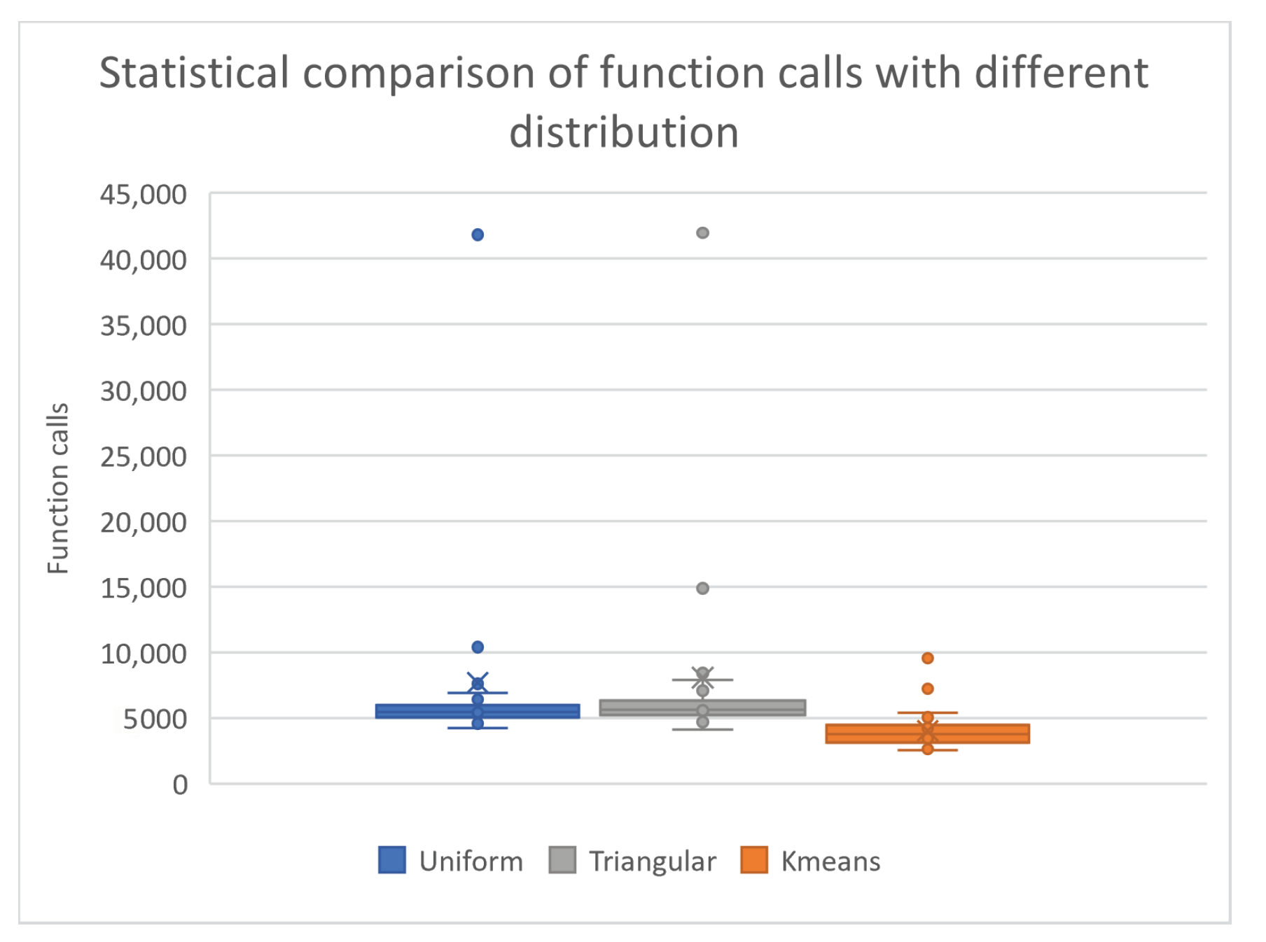
Table 2 presents the three different distributions for the initialization of the chromosomes, along with the objective function evaluations. It is evident that, with the proposed initialization, the evaluations are fewer compared to the other two initialization methods. Specifically, compared to the uniform initialization, there was a reduction of 47.88%, while in comparison to the triangular initialization, the reduction was 50.25%. As for the success rates, no significant differences were observed, and this is graphically outlined in Figure 1.
An additional set of experiments was performed to verify the reliability of the proposed technique with high-dimensional objective functions. The following functions were used:
- High conditioned elliptic function, defined as
- CM function, defined as
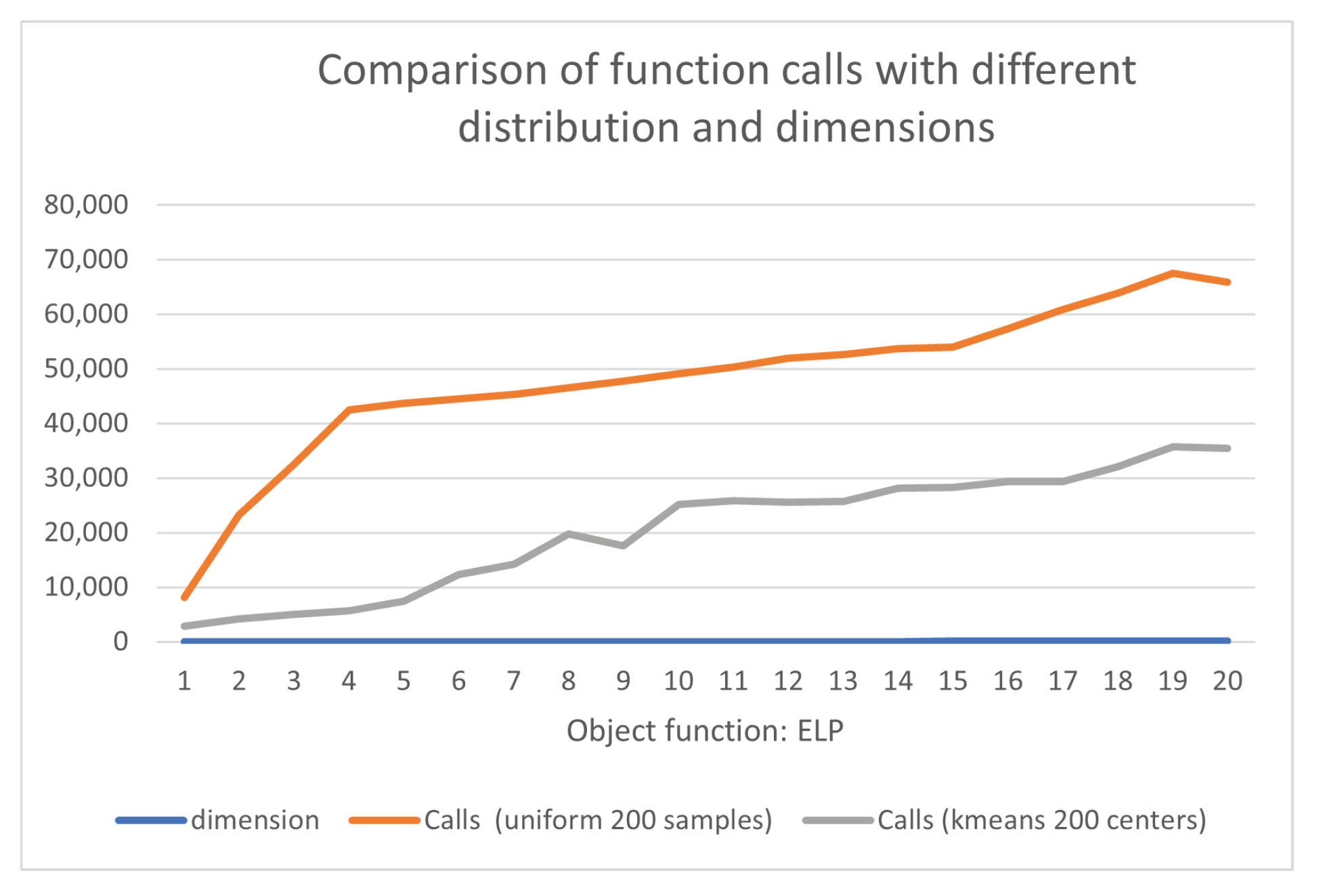
These were used as test cases in this series of experiments. For the first function, the dimension values were used, and the comparative results are outlined in Table 3 and graphically in Figure 2. It is evident that, with the proposed initialization, the results improved compared to those of the uniform distribution. Additionally, as expected, the required function evaluations increased in parallel with the dimension of the problem.
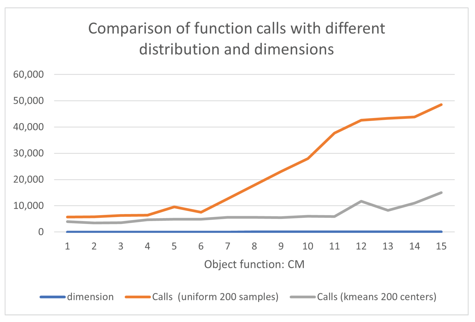
Likewise, a series of experiments was conducted for the CM function with the dimension n increased from 2 to 30, and the results are shown in Table 4 and graphically in Figure 3. The proposed initialization method requires fewer function calls to obtain the global minimum of the function, and also, the average success rate with the proposed initialization method reached 100%, whereas with the uniform distribution, it was smaller by 15%.
4. Conclusions
In this work, an innovative chromosome initialization method for genetic algorithms was proposed that utilizes the well-known k-means technique. These genetic algorithms are used to find the global minimum of multidimensional functions. This method replaces the initialization of chromosomes in genetic algorithms, which is traditionally performed by some random distribution, with centers produced by the k-means technique. In addition, in this technique, centers that are close enough are rejected from being genetic algorithm chromosomes. The above procedure significantly reduced the required number of function calls compared to random distributions, and furthermore, in difficult high-dimensional functions, it appears to be a more-efficient technique at finding the global minimum than random distributions. Future research may include the incorporation of parallel techniques such as MPI [77] or OpenMP [78] to speed up the method or application of the initialization process to other stochastic techniques such as particle swarm optimization or differential evolution.
Author Contributions
V.C., I.G.T. and V.N.S. conceived of the idea and methodology and supervised the technical part regarding the software. V.C. conducted the experiments, employing several datasets, and provided the comparative experiments. I.G.T. performed the statistical analysis. V.N.S. and all other authors prepared the manuscript. All authors have read and agreed to the published version of the manuscript.
Funding
Project name “iCREW: Intelligent small craft simulator for advanced crew training using Virtual Reality techniques” (project code:TAEDK-06195).
Institutional Review Board Statement
Not applicable.
Informed Consent Statement
Not applicable.
Data Availability Statement
Not applicable.
Acknowledgments
This research has been financed by the European Union: Next Generation EU through the Program Greece 2.0 National Recovery and Resilience Plan, under the call RESEARCH – CREATE – INNOVATE, project name “iCREW: Intelligent small craft simulator for advanced crew training using Virtual Reality techniques” (project code:TAEDK-06195).
Conflicts of Interest
The authors declare no conflict of interest.
References
- Yang, L.; Robin, D.; Sannibale, F.; Steier, C.; Wan, W. Global optimization of an accelerator lattice using multiobjective genetic algorithms. Nucl. Instruments Methods Phys. Res. Sect. A Accel. Spectrom. Detect. Assoc. Equip. 2009, 609, 50–57. [Google Scholar] [CrossRef]
- Iuliano, E. Global optimization of benchmark aerodynamic cases using physics-based surrogate models. Aerosp. Sci. Technol. 2017, 67, 273–286. [Google Scholar] [CrossRef]
- Duan, Q.; Sorooshian, S.; Gupta, V. Effective and efficient global optimization for conceptual rainfall-runoff models. Water Resour. Res. 1992, 28, 1015–1031. [Google Scholar] [CrossRef]
- Heiles, S.; Johnston, R.L. Global optimization of clusters using electronic structure methods. Int. J. Quantum Chem. 2013, 113, 2091–2109. [Google Scholar] [CrossRef]
- Shin, W.H.; Kim, J.K.; Kim, D.S.; Seok, C. GalaxyDock2: Protein–ligand docking using beta-complex and global optimization. J. Comput. Chem. 2013, 34, 2647–2656. [Google Scholar] [CrossRef]
- Liwo, A.; Lee, J.; Ripoll, D.R.; Pillardy, J.; Scheraga, H.A. Protein structure prediction by global optimization of a potential energy function. Biophysics 1999, 96, 5482–5485. [Google Scholar] [CrossRef]
- Gaing, Z.-L. Particle swarm optimization to solving the economic dispatch considering the generator constraints. IEEE Trans. Power Syst. 2003, 18, 1187–1195. [Google Scholar] [CrossRef]
- Maranas, C.D.; Androulakis, I.P.; Floudas, C.A.; Berger, A.J.; Mulvey, J.M. Solving long-term financial planning problems via global optimization. J. Econ. Dyn. Control. 1997, 21, 1405–1425. [Google Scholar] [CrossRef]
- Lee, E.K. Large-Scale Optimization-Based Classification Models in Medicine and Biology. Ann. Biomed. Eng. 2007, 35, 1095–1109. [Google Scholar] [CrossRef]
- Cherruault, Y. Global optimization in biology and medicine. Math. Comput. Model. 1994, 20, 119–132. [Google Scholar] [CrossRef]
- Wolfe, M.A. Interval methods for global optimization. Appl. Math. Comput. 1996, 75, 179–206. [Google Scholar]
- Csendes, T.; Ratz, D. Subdivision Direction Selection in Interval Methods for Global Optimization. SIAM J. Numer. Anal. 1997, 34, 922–938. [Google Scholar] [CrossRef]
- Price, W.L. Global optimization by controlled random search. J. Optim. Theory Appl. 1983, 40, 33–348. [Google Scholar] [CrossRef]
- Krivy, I.; Tvrdik, J. The controlled random search algorithm in optimizing regression models. Comput. Stat. Data Anal. 1995, 20, 229–234. [Google Scholar] [CrossRef]
- Ali, M.M.; Torn, A.; Viitanen, S. A Numerical Comparison of Some Modified Controlled Random Search Algorithms. J. Glob. Optim. 1997, 11, 377–385. [Google Scholar] [CrossRef]
- Kirkpatrick, S.; Gelatt, C.D.; Vecchi, M.P. Optimization by simulated annealing. Science 1983, 220, 671–680. [Google Scholar] [CrossRef]
- Ingber, L. Very fast simulated re-annealing. Math. Comput. Model. 1989, 12, 967–973. [Google Scholar] [CrossRef]
- Eglese, R.W. Simulated annealing: A tool for operational research. Eur. J. Oper. Res. 1990, 46, 271–281. [Google Scholar] [CrossRef]
- Storn, R.; Price, K. Differential Evolution—A Simple and Efficient Heuristic for Global Optimization over Continuous Spaces. J. Glob. Optim. 1997, 11, 341–359. [Google Scholar] [CrossRef]
- Liu, J.; Lampinen, J. A Fuzzy Adaptive Differential Evolution Algorithm. Soft Comput. 2005, 9, 448–462. [Google Scholar] [CrossRef]
- Kennedy, J.; Eberhart, R. Particle swarm optimization. In Proceedings of the ICNN’95—International Conference on Neural Networks, Perth, WA, Australia, 27 November–1 December 1995; Volume 4, pp. 1942–1948. [Google Scholar] [CrossRef]
- Poli, R.; Kennedy, J.K.; Blackwell, T. Particle swarm optimization An Overview. Swarm Intell. 2007, 1, 33–57. [Google Scholar] [CrossRef]
- Trelea, I.C. The particle swarm optimization algorithm: Convergence analysis and parameter selection. Inf. Process. Lett. 2003, 85, 317–325. [Google Scholar] [CrossRef]
- Dorigo, M.; Birattari, M.; Stutzle, T. Ant colony optimization. IEEE Comput. Intell. Mag. 2006, 1, 28–39. [Google Scholar] [CrossRef]
- Socha, K.; Dorigo, M. Ant colony optimization for continuous domains. Eur. J. Oper. Res. 2008, 185, 1155–1173. [Google Scholar] [CrossRef]
- Perez, M.; Almeida, F.; Moreno-Vega, J.M. Genetic algorithm with multistart search for the p-Hub median problem. In Proceedings of the 24th EUROMICRO Conference (Cat. No.98EX204), Vasteras, Sweden, 27 August 1998; Volume 2, pp. 702–707. [Google Scholar]
- De Oliveira, H.C.B.; Vasconcelos, G.C.; Alvarenga, G.B. A Multi-Start Simulated Annealing Algorithm for the Vehicle Routing Problem with Time Windows. In Proceedings of the 2006 Ninth Brazilian Symposium on Neural Networks (SBRN’06), Ribeirao Preto, Brazil, 23–27 October 2006; pp. 137–142. [Google Scholar]
- Liu, B.; Wang, L.; Jin, Y.H.; Tang, F.; Huang, D.X. Improved particle swarm optimization combined with chaos. Chaos Solitons Fractals 2005, 25, 1261–1271. [Google Scholar] [CrossRef]
- Shi, X.H.; Liang, Y.C.; Lee, H.P.; Lu, C.; Wang, L.M. An improved GA and a novel PSO-GA based hybrid algorithm. Inf. Process. Lett. 2005, 93, 255–261. [Google Scholar] [CrossRef]
- Garg, H. A hybrid PSO-GA algorithm for constrained optimization problems. Appl. Math. Comput. 2016, 274, 292–305. [Google Scholar] [CrossRef]
- Larson, J.; Wild, S.M. Asynchronously parallel optimization solver for finding multiple minima. Math. Program. Comput. 2018, 10, 303–332. [Google Scholar] [CrossRef]
- Bolton, H.P.J.; Schutte, J.F.; Groenwold, A.A. Multiple Parallel Local Searches in Global Optimization. In Recent Advances in Parallel Virtual Machine and Message Passing Interface, Proceedings of the EuroPVM/MPI 2000, Balatonfured, Hungary, 10–13 September 2000; Lecture Notes in Computer Science; Dongarra, J., Kacsuk, P., Podhorszki, N., Eds.; Springer: Berlin/Heidelberg, Germany, 2000; Volume 1908, p. 1908. [Google Scholar]
- Kamil, R.; Reiji, S. An Efficient GPU Implementation of a Multi-Start TSP Solver for Large Problem Instances. In Proceedings of the 14th Annual Conference Companion on Genetic and Evolutionary Computation, Philadelphia, PA, USA, 7–11 July 2012; pp. 1441–1442. [Google Scholar]
- Van Luong, T.; Melab, N.; Talbi, E.G. GPU-Based Multi-start Local Search Algorithms. In Learning and Intelligent Optimization. LION 2011; Lecture Notes in Computer Science; Coello, C.A.C., Ed.; Springer: Berlin/Heidelberg, Germany, 2011; Volume 6683. [Google Scholar] [CrossRef]
- Holland, J.H. Genetic algorithms. Sci. Am. 1992, 267, 66–73. [Google Scholar] [CrossRef]
- Stender, J. Parallel Genetic Algorithms: Theory & Applications; IOS Press: Amsterdam, The Netherlands, 1993. [Google Scholar]
- Goldberg, D. Genetic Algorithms in Search, Optimization and Machine Learning; Addison-Wesley Publishing Company: Reading, MA, USA, 1989. [Google Scholar]
- Michaelewicz, Z. Genetic Algorithms + Data Structures = Evolution Programs; Springer: Berlin/Heidelberg, Germany, 1996. [Google Scholar]
- Ansari, S.; Alnajjar, K.; Saad, M.; Abdallah, S.; Moursy, A. Automatic Digital Modulation Recognition Based on Genetic-Algorithm-Optimized Machine Learning Models. IEEE Access 2022, 10, 50265–50277. [Google Scholar] [CrossRef]
- Ji, Y.; Liu, S.; Zhou, M.; Zhao, Z.; Guo, X.; Qi, L. A machine learning and genetic algorithm-based method for predicting width deviation of hot-rolled strip in steel production systems. Inf. Sci. 2022, 589, 360–375. [Google Scholar] [CrossRef]
- Santana, Y.H.; Alonso, R.M.; Nieto, G.G.; Martens, L.; Joseph, W.; Plets, D. Indoor genetic algorithm-based 5G network planning using a machine learning model for path loss estimation. Appl. Sci. 2022, 12, 3923. [Google Scholar] [CrossRef]
- Liu, X.; Jiang, D.; Tao, B.; Jiang, G.; Sun, Y.; Kong, J.; Chen, B. Genetic algorithm-based trajectory optimization for digital twin robots. Front. Bioeng. Biotechnol. 2022, 9, 793782. [Google Scholar] [CrossRef] [PubMed]
- Nonoyama, K.; Liu, Z.; Fujiwara, T.; Alam, M.M.; Nishi, T. Energy-efficient robot configuration and motion planning using genetic algorithm and particle swarm optimization. Energies 2022, 15, 2074. [Google Scholar] [CrossRef]
- Liu, K.; Deng, B.; Shen, Q.; Yang, J.; Li, Y. Optimization based on genetic algorithms on energy conservation potential of a high speed SI engine fueled with butanol–gasoline blends. Energy Rep. 2022, 8, 69–80. [Google Scholar] [CrossRef]
- Zhou, G.; Zhu, Z.; Luo, S. Location optimization of electric vehicle charging stations: Based on cost model and genetic algorithm. Energy 2022, 247, 123437. [Google Scholar] [CrossRef]
- Chen, Q.; Hu, X. Design of intelligent control system for agricultural greenhouses based on adaptive improved genetic algorithm for multi-energy supply system. Energy Rep. 2022, 8, 12126–12138. [Google Scholar] [CrossRef]
- Min, D.; Song, Z.; Chen, H.; Wang, T.; Zhang, T. Genetic algorithm optimized neural network based fuel cell hybrid electric vehicle energy management strategy under start-stop condition. Appl. Energy 2022, 306, 118036. [Google Scholar] [CrossRef]
- Doewes, R.I.; Nair, R.; Sharma, T. Diagnosis of COVID-19 through blood sample using ensemble genetic algorithms and machine learning classifier. World J. Eng. 2022, 19, 175–182. [Google Scholar] [CrossRef]
- Choudhury, S.; Rana, M.; Chakraborty, A.; Majumder, S.; Roy, S.; RoyChowdhury, A.; Datta, S. Design of patient specific basal dental implant using Finite Element method and Artificial Neural Network technique. J. Eng. Med. 2022, 236, 1375–1387. [Google Scholar] [CrossRef]
- El-Anwar, M.I.; El-Zawahry, M.M. A three dimensional finite element study on dental implant design. J. Genet. Eng. Biotechnol. 2011, 9, 77–82. [Google Scholar] [CrossRef]
- Zheng, Q.; Zhong, J. Design of Automatic Pronunciation Error Correction System for Cochlear Implant Based on Genetic Algorithm. In Proceedings of the ICMMIA: Application of Intelligent Systems in Multi-Modal Information Analytics 2022, Online, 23 April 2022; pp. 1041–1047. [Google Scholar]
- Brahim, O.; Hamid, B.; Mohammed, N. Optimal design of inductive coupled coils for biomedical implants using metaheuristic techniques. E3S Web Conf. 2022, 351, 01063. [Google Scholar] [CrossRef]
- Tokgoz, E.; Carro, M.A. Applications of Artificial Intelligence, Machine Learning, and Deep Learning on Facial Plastic Surgeries; Springer: Cham, Switzerland, 2023; pp. 281–306. [Google Scholar]
- Wang, B.; Gomez-Aguilar, J.F.; Sabir, Z.; Raja, M.A.Z.; Xia, W.; Jahanshahi, H.; Alassafi, M.O.; Alsaadi, F. Surgery Using The Capability Of Morlet Wavelet Artificial Neural Networks. Fractals 2023, 30, 2240147. [Google Scholar] [CrossRef]
- Ahmed, M.; Seraj, R.; Islam, S.M.S. The k-means algorithm: A comprehensive survey and performance evaluation. Electronics 2020, 9, 1295. [Google Scholar] [CrossRef]
- Maaranen, H.; Miettinen, K.; Makela, M.M. Quasi-random initial population for genetic algorithms. Comput. Math. Appl. 2004, 47, 1885–1895. [Google Scholar] [CrossRef]
- Paul, P.V.; Dhavachelvan, P.; Baskaran, R. A novel population initialization technique for Genetic Algorithm. In Proceedings of the 2013 International Conference on Circuits, Power and Computing Technologies (ICCPCT), Nagercoil, India, 20–21 March 2013; pp. 1235–1238. [Google Scholar]
- Li, C.; Chu, X.; Chen, Y.; Xing, L. A knowledge-based technique for initializing a genetic algorithm. J. Intell. Fuzzy Syst. 2016, 31, 1145–1152. [Google Scholar] [CrossRef]
- Hassanat, A.B.; Prasath, V.S.; Abbadi, M.A.; Abu-Qdari, S.A.; Faris, H. An improved genetic algorithm with a new initialization mechanism based on regression techniques. Information 2018, 9, 167. [Google Scholar] [CrossRef]
- Kaelo, P.; Ali, M.M. Integrated crossover rules in real coded genetic algorithms. Eur. J. Oper. Res. 2007, 176, 60–76. [Google Scholar] [CrossRef]
- Tsoulos, I.G. Modifications of real code genetic algorithm for global optimization. Appl. Math. Comput. 2008, 203, 598–607. [Google Scholar] [CrossRef]
- Powell, M.J.D. A Tolerant Algorithm for Linearly Constrained Optimization Calculations. Math. Program. 1989, 45, 547–566. [Google Scholar] [CrossRef]
- Beyer, H.G.; Schwefel, H.P. Evolution strategies–A comprehensive introduction. Nat. Comput. 2002, 1, 3–52. [Google Scholar] [CrossRef]
- LeCun, Y.; Bengio, Y.; Hinton, G. Deep learning. Nature 2015, 521, 436–444. [Google Scholar] [CrossRef] [PubMed]
- Whitley, D. The GENITOR algorithm and selection pressure: Why rank-based allocation of reproductive trials is best. In Proceedings of the Third International Conference on Genetic Algorithms, Fairfax, VA, USA, 4–7 June 1989; pp. 116–121. [Google Scholar]
- Eiben, A.E.; Smith, J.E. Introduction to Evolutionary Computing; Springer: Berlin/Heidelberg, Germany, 2015. [Google Scholar]
- Lloyd, S. Least squares quantization in PCM. IEEE Trans. Inf. Theory 1982, 28, 129–137. [Google Scholar] [CrossRef]
- MacQueen, J.B. Some Methods for classification and Analysis of Multivariate Observations. In Proceedings of the 5th Berkeley Symposium on Mathematical Statistics and Probability, Oakland, CA, USA, 21 June–18 July 1967; pp. 281–297. [Google Scholar]
- Jain, A.K.; Murty, M.N.; Flynn, P.J. Data clustering: A review. Acm Comput. Surv. 1999, 31, 264–323. [Google Scholar] [CrossRef]
- Bishop, C.M. Pattern Recognition and Machine Learning; Springer: Berlin/Heidelberg, Germany, 2006. [Google Scholar]
- Hastie, T.; Tibshirani, R.; Friedman, J. The Elements of Statistical Learning: Data Mining, Inference, and Prediction; Springer: Berlin/Heidelberg, Germany, 2009. [Google Scholar]
- Ali, M.M.; Khompatraporn, C.; Zabinsky, Z.B. A Numerical Evaluation of Several Stochastic Algorithms on Selected Continuous Global Optimization Test Problems. J. Glob. Optim. 2005, 31, 635–672. [Google Scholar] [CrossRef]
- Floudas, C.A.; Pardalos, P.M.; Adjiman, C.; Esposoto, W.; Gümüs, Z.; Harding, S.; Klepeis, J.; Meyer, C.; Schweiger, C. Handbook of Test Problems in Local and Global Optimization; Kluwer Academic Publishers: Dordrecht, The Netherland, 1999. [Google Scholar]
- Gaviano, M.; Ksasov, D.E.; Lera, D.; Sergeyev, Y.D. Software for generation of classes of test functions with known local and global minima for global optimization. Acm Trans. Math. Softw. 2003, 29, 469–480. [Google Scholar] [CrossRef]
- Lennard-Jones, J.E. On the Determination of Molecular Fields. Proc. R. Soc. Lond. A 1924, 106, 463–477. [Google Scholar]
- Stein, W.E.; Keblis, M.F. A new method to simulate the triangular distribution. Math. Comput. Model. 2009, 49, 1143–1147. [Google Scholar] [CrossRef]
- Gropp, W.; Lusk, E.; Doss, N.; Skjellum, A. A high-performance, portable implementation of the MPI message passing interface standard. Parallel Comput. 1996, 22, 789–828. [Google Scholar] [CrossRef]
- Chandra, R.; Dagum, L.; Kohr, D.; Maydan, D.; McDonald, J.; Menon, R. Parallel Programming in OpenMP; Morgan Kaufmann Publishers Inc.: Cambridge, MA, USA, 2001. [Google Scholar]
Figure 1.
Statistical comparison of function calls with different distributions.

Figure 2.
Comparison of function calls of ELP function with different distributions and dimensions.

Figure 3.
Comparison of function calls of CM function with different distributions and dimensions.

Table 2.
Comparison of function calls and success rates with different distributions. The fractions in parentheses indicate percentage of runs where the global optimum was successfully discovered. When this fraction is absent, it is an indication that the global minimum was discovered in every execution (100% success).
| Problem | Uniform | Triangular | Kmeans |
|---|---|---|---|
| BF1 | 5731 | 5934 | 4478 |
| BF2 | 5648 (0.97) | 5893 | 4512 |
| BRANIN | 4680 | 4835 | 4627 |
| CM4 | 5801 | 5985 | 4431 |
| CAMEL | 4965 | 5099 | 4824 |
| EASOM | 5657 | 7089 | 4303 |
| EXP4 | 4934 | 4958 | 4539 |
| EXP8 | 5021 | 5187 | 4689 |
| EXP16 | 5063 | 5246 | 4874 |
| EXP32 | 5044 | 5244 | 5016 |
| GKLS250 | 4518 | 4710 | 4525 |
| GKLS350 | 4650 | 4833 | 4637 |
| GOLDSTEIN | 8099 | 8537 | 7906 |
| GRIEWANK2 | 5500 (0.97) | 5699 (0.97) | 4324 |
| GRIEWANK10 | 6388 (0.70) | 7482 (0.63) | 4559 |
| HANSEN | 5681 (0.93) | 6329 | 6357 |
| HARTMAN3 | 4950 | 5157 | 4998 |
| HARTMAN6 | 5288 | 5486 | 5258 |
| POTENTIAL3 | 5587 | 5806 | 5604 |
| POTENTIAL5 | 7335 | 7824 | 7450 |
| RASTRIGIN | 5703 | 5848 | 4481 |
| ROSENBROCK4 | 4241 | 4441 | 4241 |
| ROSENBROCK8 | 41,802 | 41,965 | 4523 |
| ROSENBROCK16 | 42,196 | 42,431 | 4962 |
| SHEKEL5 | 5488 (0.97) | 5193 (0.97) | 5232 (0.97) |
| SHEKEL7 | 5384 | 5711 (0.97) | 5695 (0.97) |
| SHEKEL10 | 6360 | 5989 | 6396 |
| TEST2N4 | 5000 | 5179 | 5047 |
| TEST2N5 | 5306 | 5309 | 5039 |
| TEST2N6 | 5245 | 5492 | 5107 |
| TEST2N7 | 5282 (0.93) | 5583 | 5216 |
| SINU4 | 4844 | 5046 | 4899 |
| SINU8 | 5368 | 5503 | 5509 |
| SINU16 | 6919 | 5583 | 5977 |
| TEST30N3 | 7215 | 8115 | 5270 |
| TEST30N4 | 7073 | 7455 | 6712 |
| Total | 273,966 (0.98) | 282,176 (0.985) | 186,217 (0.998) |
Table 3.
Objective function ELP. Comparison of function calls with different distributions and dimensions.
Table 3.
Objective function ELP. Comparison of function calls with different distributions and dimensions.
| Dimension | Calls (200 Uniform Samples) | Calls (200 k-Means Centers) |
|---|---|---|
| 5 | 15,637 | 4332 |
| 10 | 24,690 | 4486 |
| 15 | 39,791 | 4743 |
| 20 | 42,976 | 5194 |
| 25 | 43,617 | 7152 |
| 30 | 44,502 | 6914 |
| 35 | 45,252 | 15,065 |
| 40 | 46,567 | 13,952 |
| 45 | 47,640 | 15,193 |
| 50 | 49,393 | 22,535 |
| 55 | 50,062 | 23,692 |
| 60 | 52,293 | 25,570 |
| 65 | 52,546 | 25,678 |
| 70 | 53,346 | 28,153 |
| 75 | 54,110 | 28,328 |
| 80 | 57,209 | 29,320 |
| 85 | 60,970 | 29,371 |
| 90 | 65,319 | 32,121 |
| 95 | 68,097 | 35,721 |
| 100 | 66,803 | 35,396 |
| Total | 980,820 | 392,916 |
Table 4.
Objective function CM. Comparison of function calls and success rates using different distributions.The fractions in parentheses indicate percentage of runs where the global optimum was successfully discovered. When this fraction is absent, it is an indication that the global minimum was discovered in every execution (100% success).
| Dimension | Calls (200 Uniform Samples) | Calls (200 k-Means Centers) |
|---|---|---|
| 2 | 5665 | 4718 |
| 4 | 6212 | 4431 |
| 6 | 7980 | 4390 |
| 8 | 9917 | 4449 |
| 10 | 12,076 (0.97) | 4481 |
| 12 | 14,672 | 4565 |
| 14 | 18,708 (0.87) | 4685 |
| 16 | 23,251 (0.77) | 4687 |
| 18 | 24,624 (0.77) | 4766 |
| 20 | 30,153 (0.80) | 4848 |
| 22 | 35,851 (0.77) | 15,246 (0.97) |
| 24 | 43,677 (0.93) | 7865 (0.93) |
| 26 | 41,492 (0.77) | 5627 |
| 28 | 38,017 (0.73) | 10,566 (0.97) |
| 30 | 47,538 (0.83) | 24,803 (0.90) |
| Total | 359,833 (0.84) | 110,127 (0.98) |
Disclaimer/Publisher’s Note: The statements, opinions and data contained in all publications are solely those of the individual author(s) and contributor(s) and not of MDPI and/or the editor(s). MDPI and/or the editor(s) disclaim responsibility for any injury to people or property resulting from any ideas, methods, instructions or products referred to in the content. |
© 2023 by the authors. Licensee MDPI, Basel, Switzerland. This article is an open access article distributed under the terms and conditions of the Creative Commons Attribution (CC BY) license (https://creativecommons.org/licenses/by/4.0/).
Share and Cite
MDPI and ACS Style
Charilogis, V.; Tsoulos, I.G.; Stavrou, V.N. An Intelligent Technique for Initial Distribution of Genetic Algorithms. Axioms 2023, 12, 980. https://0-doi-org.brum.beds.ac.uk/10.3390/axioms12100980
AMA Style
Charilogis V, Tsoulos IG, Stavrou VN. An Intelligent Technique for Initial Distribution of Genetic Algorithms. Axioms. 2023; 12(10):980. https://0-doi-org.brum.beds.ac.uk/10.3390/axioms12100980
Chicago/Turabian StyleCharilogis, Vasileios, Ioannis G. Tsoulos, and V. N. Stavrou. 2023. "An Intelligent Technique for Initial Distribution of Genetic Algorithms" Axioms 12, no. 10: 980. https://0-doi-org.brum.beds.ac.uk/10.3390/axioms12100980
Note that from the first issue of 2016, this journal uses article numbers instead of page numbers. See further details here.