Abundant Solitary Wave Solutions for the Boiti–Leon–Manna–Pempinelli Equation with M-Truncated Derivative

Abstract

In this work, we consider the Boiti–Leon–Manna–Pempinelli equation with the M-truncated derivative (BLMPE-MTD). Our aim here is to obtain trigonometric, rational and hyperbolic solutions of BLMPE-MTD by employing two diverse methods, namely, He’s semi-inverse method and the extended tanh function method. In addition, we generalize some previous results. As the Boiti–Leon–Manna–Pempinelli equation is a model for an incompressible fluid, the solutions obtained may be utilized to represent a wide variety of fascinating physical phenomena. We construct a large number of 2D and 3D figures to demonstrate the impact of the M-truncated derivative on the exact solution of the BLMPE-MTD.

1. Introduction

Mathematical models are the most accurate approach to describe nonlinear physical events. Partial differential equations (PDEs) have been modeled in order to investigate and learn more about the structure of physical phenomena. One of the most important physical challenges for these models is the need to solve the issue of traveling waves. This has made the development of mathematical techniques for generating accurate solutions to PDEs a substantial and crucial endeavor in the field of nonlinear sciences. Recently, a wide range of approaches, such as $(G^{\prime }/G)$-expansion [1,2], the mapping method [3], Jacobi elliptic function [4,5], Sardar-subequation method [6], Exp-function method [7], sine-Gordon expansion [8],$exp(-\varphi (\varsigma \left)\right)$-expansion [9], extended trial equation [10], tanh-sech [11,12], F-expansion approach [13], homotopy perturbation technique [14], He’s semi-inverse method [15], etc., have been offered as potential solutions to the problem of PDEs.

On the other hand, a larger variety of physical problems needed more complicated mathematical differentiation operators. A novel differentiation notion has emerged that combines the ideas of fractional differentiation and fractal derivative. Therefore, different forms of fractional derivatives were presented by several mathematicians. The most well-known ones are the ones proposed by Riesz, Marchaud, Kober, Riemann–Liouville, Erdelyi, Hadamard, Grunwald–Letnikov, and Caputo [16,17,18,19]. The majority of fractional derivative kinds do not adhere to the traditional derivative formulae, such as the chain rule, quotient rule, and product rule. Recently, a new derivative, referred to as the M-truncated derivative (MTD) which is a natural extension of the classical derivative, was presented by Sousa et al. [20]. The MTD of order $\gamma \in (0,1]$ for $u:[0,\infty )\to \mathbb{R}$ is defined as:

$${\mathcal{M}}_{i,t}^{\gamma ,\beta }u\left(t\right)=\underset{h\to 0}{lim}\frac{u\left(t{\mathcal{E}}_i^{\beta }\left(h{t}^{-\gamma }\right)\right)-u\left(t\right)}{h},$$

where ${}_i{\mathcal{E}}_{\beta }\left(z\right),$ for $z\in \mathbb{C}$ and $\beta >0$, is the truncated Mittag-Leffler function and is defined as:

$${\mathcal{E}}_i^{\beta }\left(z\right)=\sum _{k=0}^i\frac{z^k}{\Gamma (\beta k+1)}.$$

For any real numbers a and $b$, the following properties of the MTD are satisfying [20]:

(1)

${\mathcal{M}}_{i,z}^{\gamma ,\beta }(au+bv)=a{\mathcal{M}}_{i,z}^{\gamma ,\beta }\left(u\right)+b{\mathcal{M}}_{i,z}^{\gamma ,\beta }\left(v\right),$

(2)

${\mathcal{M}}_{i,z}^{\gamma ,\beta }(u\circ v)\left(z\right)=u^{{}^{\prime }}\left(v\left(z\right)\right){\mathcal{M}}_{i,z}^{\gamma ,\beta }v\left(z\right),$

(3)

${\mathcal{M}}_{i,z}^{\gamma ,\beta }\left(uv\right)=u{\mathcal{M}}_{i,z}^{\gamma ,\beta }v+v{\mathcal{M}}_{i,z}^{\gamma ,\beta }u,$

(4)

${\mathcal{M}}_{i,z}^{\gamma ,\beta }u)\left(z\right)=\frac{z^{1-\gamma }}{\Gamma (\beta +1)}\frac{du}{dz},$

(5)

${\mathcal{M}}_{i,z}^{\gamma ,\beta }\left(z^{\nu }\right)=\frac{\nu }{\Gamma (\beta +1)}{z}^{\nu -\gamma }.$

Recently, a large number of authors have examined several forms of evolution equations with M-truncated derivative see for instance [21,22,23,24,25] and the references therein. The $(3+1)$-dimensional Boiti–Leon–Manna–Pempinelli equation (BLMPE), which represents the propagation of a fluid and may be thought of as a model for incompressible fluid, is one of the most well-known evolution equations. In this paper, we consider BLMPE with M-truncated derivative (BLMPE-MTD) as follows [26,27]:

$${\mathcal{M}}_{i,t}^{\gamma ,\beta }({\mathcal{Y}}_y+{\mathcal{Y}}_z)+{\mathcal{Y}}_{yxxx}+{\mathcal{Y}}_{zxxx}-3{\left({\mathcal{Y}}_x({\mathcal{Y}}_y+{\mathcal{Y}}_z)\right)}_x=0.$$

(1)

In addition, this Equation (1) explains the interaction of the Riemann wave propagating along the y-axis and a long wave propagating along the x-axis when $z=0$. Several researchers have investigated various analytical solutions to Equation (1) with $\gamma =1$ and $\beta =0$, including modified hyperbolic tangent function [28], general bilinear form [29], Hirota’s bilinear and extended three-wave approach [30], $(G^{\prime }/G)$-expansion [31], ansatz functions, the bilinear form, and extended homoclinic test technique [32], auxiliary equation method [33], Hirota’s direct method [34], modified exponential function [35], Bäcklund transformation method [36], extended tanh function [37], and modified Kudryashov method, ($1/G^{\prime }$)-expansion method [38], and the extended transformed rational function [39]. Moreover, the exact solutions of fractional BLMPE with conformable derivative has attained by modified Kudryashov, generalized $(G^{\prime }/G)$-expansion and $exp(-\varphi )$-expansion methods [40]. While, the solutions of BLMPE (1) with a M-truncated derivative are not yet achieved.

Our purpose of this study is to acquire the analytical solutions of BLMPE-MTD (1). We employ two diverse methods, namely, He’s semi-inverse method and the extended tanh function method to obtain these solutions. The proposed methods are effective and also can be used for many other nonlinear evolution equations. In addition, we generalize some prior findings, including those found in [37]. Because of the M–turncated derivative exists in Equation (1), the solutions are very useful for characterizing various important physical processes, which is why they are so popular among physics researchers (1). We also use the MATLAB program to offer a wide variety of graphs for analyzing how the M-turncated derivative modifies the exact solutions to the BLMPE-MTD (1).

The following is a brief synopsis of the contents of this article: The wave equation for BLMPE-MTD (1) is derived in Section 2. In Section 3, we use He’s semi-inverse and extended tanh function approaches to obtain exact solutions to the BLMPE-MTD. In Section 4, we present some graphical representation. In the last section, the paper’s conclusions are presented.

2. Exact Solutions of BLMPE-MTD

The BLMPE-MTD wave Equation (1) is produced using the next wave transformation:

$$\mathcal{Y}(x,y,z,t)=\mathcal{H}\left(\mu \right),\mu ={\mu }_{1}x+{\mu }_{2}y+{\mu }_{3}z+\frac{{\mu }_4\Gamma (\beta +1)}{\gamma }{t}^{\gamma },$$

(2)

where $\mathcal{H}$ is the unknown function, ${\mu }_1,{\mu }_2,$ ${\mu }_3$ and ${\mu }_4$ are parameters to be calculated. We can see that

$$\begin{array}{ccc}\hfill {\mathcal{Y}}_x& =& {\mu }_1{\mathcal{H}}^{\prime },{\mathcal{Y}}_{xx}={\mu }_1^2{\mathcal{H}}^{″},{\mathcal{Y}}_z={\mu }_3{\mathcal{H}}^{\prime },\hfill \\ \hfill {\mathcal{Y}}_{zx}& =& {\mu }_1{\mu }_3{\mathcal{H}}^{″},{\mathcal{Y}}_{yxxx}={\mu }_2{\mu }_1^3{\mathcal{H}}^{⁗},\hfill \\ \hfill {\mathcal{Y}}_{zxxx}& =& {\mu }_3{\mu }_1^3{\mathcal{H}}^{⁗},{\mathcal{M}}_{i,t}^{\gamma ,\beta }({\mathcal{Y}}_y+{\mathcal{Y}}_z)={\mu }_4({\mu }_2+{\mu }_3){\mathcal{H}}^{″}.\hfill \end{array}$$

(3)

Plugging Equation (3) into Equation (1), we have

$${\mathcal{H}}^{⁗}+{\hslash }_1{\mathcal{H}}^{″}+2{\hslash }_2{\mathcal{H}}^{\prime }{\mathcal{H}}^{″}=0,$$

(4)

where

$${\hslash }_1=\frac{{\mu }_4}{{\mu }_1^3}\mathrm{and}{\hslash }_2=\frac{-3}{{\mu }_1}.$$

Integrating Equation (4) and omitting the integral constant, we obtain

$${\mathcal{H}}^{‴}+{\hslash }_1{\mathcal{H}}^{\prime }+{\hslash }_2{\left({\mathcal{H}}^{\prime }\right)}^2=0.$$

(5)

In the following, we use the He’s semi-inverse method and extended tanh function method to acquire the solution of the wave Equation (5). After that, we use (2) to find the solutions of the BLMPE-MTD (1).

2.1. He’s Semi-Inverse Method

The next variational formulations are obtained by applying He’s semi-inverse approach from [41,42,43]:

$$\mathcal{J}\left(\mathcal{H}\right)={\int }_0^{\infty }\{\frac{1}{2}{\left({\mathcal{H}}^{\prime \prime }\right)}^2-\frac{1}{2}{\hslash }_1{\left({\mathcal{H}}^{\prime }\right)}^2+\frac{1}{3}{\hslash }_2{\left({\mathcal{H}}^{\prime }\right)}^3\}d\mu .$$

(6)

According to [44], let the solution of Equation (6) be

$$\mathcal{H}\left(\mu \right)=\mathcal{K}\sec \mathrm{h}\left(\mu \right),$$

(7)

where the constant $\mathcal{K}$ is unknown. Putting Equation (7) into Equation (6) we attain

$$\begin{array}{ccc}\hfill \mathcal{J}& =& \frac{1}{2}{\mathcal{K}}^2{\int }_0^{\infty }[{\sec \mathrm{h}}^2\left(\mu \right){tanh}^4\left(\mu \right)+{\sec \mathrm{h}}^4\left(\mu \right){tanh}^2\left(\mu \right)+{\sec \mathrm{h}}^6\left(\mu \right)\hfill \\ & & -{\hslash }_1{\sec \mathrm{h}}^2\left(\mu \right){tanh}^2\left(\mu \right)+\frac{2}{3}{\hslash }_2\mathcal{K}{\sec \mathrm{h}}^3\left(\mu \right){tanh}^3\left(\mu \right)]d\mu \hfill \\ & =& \frac{1}{2}{\mathcal{K}}^2{\int }_0^{\infty }[({\sec \mathrm{h}}^2\left(\mu \right)-{\hslash }_1{\sec \mathrm{h}}^2\left(\mu \right){tanh}^2\left(\mu \right)+\frac{2}{3}{\hslash }_2\mathcal{K}{\sec \mathrm{h}}^3\left(\mu \right){tanh}^3\left(\mu \right)]d\mu \hfill \\ & =& \frac{{\mathcal{K}}^2}{2}-{\hslash }_1\frac{{\mathcal{K}}^2}{6}-\frac{2}{45}{\hslash }_2{\mathcal{K}}^3.\hfill \end{array}$$

Making $\mathcal{J}$ stationary relative to $\mathcal{K}$

$$\frac{\partial \mathcal{J}}{\partial \mathcal{K}}=(1-\frac{1}{3}{\hslash }_1)\mathcal{K}-\frac{2}{15}{\hslash }_2{\mathcal{K}}^2=0.$$

(8)

Equation (8) may be solved, leading to

$$\mathcal{K}=\frac{15-5{\hslash }_1}{2{\hslash }_2}.$$

Hence, Equation (4) has the solution

$$\mathcal{H}\left(\mu \right)=\frac{15-5{\hslash }_1}{6{\hslash }_2}\sec \mathrm{h}\left(\mu \right).$$

Now, solution of BLMPE-MTD (1) is

$$\mathcal{Y}(x,y,z,t)=\frac{15-5{\hslash }_1}{2{\hslash }_2}\sec \mathrm{h}({\mu }_{1}x+{\mu }_{2}y+{\mu }_{3}z+\frac{{\mu }_4\Gamma (\beta +1)}{\gamma }{t}^{\gamma }).$$

(9)

Similarly, we may think about the solution to Equation (4) as

$$\mathcal{H}\left(\mu \right)=\mathcal{B}\sec \mathrm{h}\left(\mu \right){tanh}^2\left(\mu \right).$$

When we repeat the previous procedures, we end with

$$\mathcal{B}=\frac{11(1199-213{\hslash }_1)}{1456{\hslash }_2}.$$

Hence, the solutions of BLMPE-MTD (1) is

$$\mathcal{Y}(x,y,z,t)=\frac{11(1199-213{\hslash }_1)}{1456{\hslash }_2}\sec \mathrm{h}\left(\mu \right){tanh}^2\left(\mu \right),$$

(10)

where $\mu ={\mu }_{1}x+{\mu }_{2}y+{\mu }_{3}z+\frac{{\mu }_4\Gamma (\beta +1)}{\gamma }{t}^{\gamma }.$

2.2. Extended Tanh Function Method

Let us suppose the solution $\mathcal{H}$ of Equation (5) is (for more detail, see [45]):

$$\mathcal{H}\left(\mu \right)=A_0+\sum _{k=1}^N(A_k{\mathcal{Z}}^k+\frac{B_k}{{\mathcal{Z}}^k}),$$

(11)

where $\mathcal{Z}$ solves the Riccati equation

$${\mathcal{Z}}^{\prime }={\mathcal{Z}}^2+\vartheta ,$$

(12)

with $\vartheta$ is a real constant. By using homogeneous balancing between ${\left({\mathcal{H}}^{\prime }\right)}^2$ with ${\mathcal{H}}^{‴}$ in Equation (5), we deduce that

$$2N+N=N+3⟹N=1.$$

Hence, Equation (11) becomes:

$$\mathcal{H}\left(\mu \right)=A_0+A_1\mathcal{Z}+\frac{B_1}{\mathcal{Z}}.$$

(13)

Equation (12) has the following solutions:

$$\mathcal{Z}\left(\mu \right)=\sqrt{\vartheta }tan\left(\sqrt{\vartheta }\mu \right)\mathrm{or}\mathcal{Z}\left(\mu \right)=-\sqrt{\vartheta }cot\left(\sqrt{\vartheta }\mu \right),$$

(14)

if $\vartheta >0,$ or

$$\mathcal{Z}\left(\mu \right)=-\sqrt{-\vartheta }tanh\left(\sqrt{-\vartheta }\mu \right)\mathrm{or}\mathcal{Z}\left(\mu \right)=-\sqrt{-\vartheta }coth\left(\sqrt{-\vartheta }\mu \right),$$

(15)

if $\vartheta <0,$ or

$$\mathcal{Z}\left(\mu \right)=\frac{-1}{\mu },$$

(16)

if $\vartheta =0.$

• Plugging Equation (13) into Equation (5) yields

$$\begin{array}{ccc}& & (6A_1+{\hslash }_2{A}_1^2){\mathcal{Z}}^4+(8\vartheta A_1+{\hslash }_1{A}_1+2\vartheta A_1^2{\hslash }_2-B_1{A}_1{\hslash }_2){\mathcal{Z}}^2\hfill \\ & & +(2{\vartheta }^2{A}_1-2B_1\vartheta -{\hslash }_1{B}_1+\vartheta {\hslash }_1{A}_1-4{\hslash }_2{A}_1{B}_1\vartheta +{\vartheta }^2{\hslash }_2{A}_1^2+{\hslash }_2{B}_1^2)\hfill \\ & & +\vartheta B_1(-8\vartheta -{\hslash }_1-\vartheta A_1{\hslash }_2+2{\hslash }_2{B}_1){\mathcal{Z}}^{-2}+{\vartheta }^2{B}_1({\hslash }_2{B}_1-6\vartheta ){\mathcal{Z}}^{-4}=0.\hfill \end{array}$$

Putting each coefficients ${\mathcal{Z}}^k$ to zero

$$6A_1+{\hslash }_2{A}_1^2=0,$$

$$A_1(8\vartheta +{\hslash }_1+2\vartheta A_1{\hslash }_2-B_1{\hslash }_2)=0,$$

$$2{\vartheta }^2{A}_1-2B_1\vartheta -{\hslash }_1{B}_1+\vartheta {\hslash }_1{A}_1-4{\hslash }_2{A}_1{B}_1\vartheta +{\vartheta }^2{\hslash }_2{A}_1^2+{\hslash }_2{B}_1^2=0,$$

$$\vartheta B_1(-8\vartheta -{\hslash }_1-\vartheta A_1{\hslash }_2+2{\hslash }_2{B}_1)=0,$$

and

$${\vartheta }^2{B}_1({\hslash }_2{B}_1-6\vartheta )=0.$$

We receive three sets after solving these equations:

• First set:

$$A_0=\mathrm{Free},A_1=2{\mu }_1,B_1=0,\mathrm{and}{\mu }_4=4\vartheta {\mu }_1^3.$$

(17)

• Second set:

$$A_0=\mathrm{Free},A_1=0,B_1=-2\vartheta {\mu }_1,\mathrm{and}{\mu }_4=4\vartheta {\mu }_1^3.$$

(18)

• Third set:

$$A_0=\mathrm{Free},A_1=2{\mu }_1,B_1=-2\vartheta {\mu }_1,\mathrm{and}{\mu }_4=16\vartheta {\mu }_1^3.$$

(19)

• First set: The Equation (5) has the solution

$$\mathcal{H}\left(\mu \right)=A_0+2{\mu }_1\mathcal{Z}\left(\mu \right).$$

There are three possible situations for $\mathcal{Z}\left(\mu \right)$:

Case 1: If $\vartheta >0,$ then we obtain by using (14)

$$\mathcal{H}\left(\mu \right)=A_0+2{\mu }_1\sqrt{\vartheta }tan\left(\sqrt{\vartheta }\mu \right),$$

and

$$\mathcal{H}\left(\mu \right)=A_0-2{\mu }_1\sqrt{\vartheta }cot\left(\sqrt{\vartheta }\mu \right).$$

Consequently, the solutions of BLMPE-MTD (1) are

$$\mathcal{Y}(x,y,z,t)=A_0+2{\mu }_1\sqrt{\vartheta }tan\left(\sqrt{\vartheta }\mu \right),$$

(20)

and

$$\mathcal{Y}(x,y,z,t)=A_0-2{\mu }_1\sqrt{\vartheta }cot\left(\sqrt{\vartheta }\mu \right),$$

(21)

where $\mu ={\mu }_{1}x+{\mu }_{2}y+{\mu }_{3}z+\frac{\Gamma (\beta +1)}{\gamma }\left(4{\mu }_1^3\right)t^{\gamma }.$

Case 2: If $\vartheta <0,$ then we obtain by using (15)

$$\mathcal{H}\left(\mu \right)=A_0-2{\mu }_1\sqrt{-\vartheta }tanh\left(\sqrt{-\vartheta }\mu \right),$$

and

$$\mathcal{H}\left(\mu \right)=A_0-2{\mu }_1\sqrt{-\vartheta }coth\left(\sqrt{-\vartheta }\mu \right).$$

Consequently, the solutions of BLMPE-MTD (1) are

$$\mathcal{Y}(x,y,z,t)=A_0-2{\mu }_1\sqrt{-\vartheta }tanh\left(\sqrt{-\vartheta }\mu \right),$$

(22)

and

$$\mathcal{Y}(x,y,z,t)=A_0-2{\mu }_1\sqrt{-\vartheta }coth\left(\sqrt{-\vartheta }\mu \right),$$

(23)

where $\mu ={\mu }_{1}x+{\mu }_{2}y+{\mu }_{3}z+\frac{4\vartheta {\mu }_1^3\Gamma (\beta +1)}{\gamma }{t}^{\gamma }.$

Case 3: If $\vartheta =0,$ then we obtain by using (16)

$$\mathcal{H}\left(\mu \right)=A_0-\frac{2{\mu }_1}{\mu }.$$

Consequently, the solutions of BLMPE-MTD (1) are

$$\mathcal{Y}(x,y,z,t)=A_0-\frac{2{\mu }_1}{\mu },$$

(24)

where $\mu ={\mu }_{1}x+{\mu }_{2}y+{\mu }_{3}z+\frac{4{\mu }_1^3\Gamma (\beta +1)}{\gamma }{t}^{\gamma }.$

• Second set: When $\vartheta >0$ and $\vartheta <0,$ the solutions are identical to those in the first set. If $\vartheta =0$, the solution of BLMPE-MTD (1) is

$$\mathcal{Y}(x,y,z,t)=A_0.$$

(25)

• Third set: The solution of Equation (5) is

$$\mathcal{H}\left(\mu \right)=A_0+2{\mu }_1\mathcal{Z}\left(\mu \right)-\frac{2{\mu }_1\vartheta }{\mathcal{Z}\left(\mu \right)}.$$

There are three possible situations for $\mathcal{Z}\left(\mu \right)$:

Case 1: If $\vartheta >0,$ then by using (14) we obtain

$$\mathcal{H}\left(\mu \right)=A_0+2{\mu }_1\sqrt{\vartheta }[tan\left(\sqrt{\vartheta }\mu \right)-cot\left(\sqrt{\vartheta }\mu \right)].$$

Consequently, the solutions of BLMPE-MTD (1) are

$$\mathcal{Y}(x,y,z,t)=A_0+2{\mu }_1\sqrt{\vartheta }(tan\left(\sqrt{\vartheta }\mu \right)-cot\left(\sqrt{\vartheta }\mu \right)).$$

(26)

Case 2: If $\vartheta <0,$ then by using (15) we have

$$\mathcal{H}\left(\mu \right)=A_0-2{\mu }_1\sqrt{-\vartheta }(tanh\left(\sqrt{-\vartheta }\mu \right)+coth\left(\sqrt{-\vartheta }\mu \right)).$$

Consequently, the solutions of BLMPE-MTD (1) are

$$\mathcal{Y}(x,y,z,t)=A_0-2{\mu }_1\sqrt{-\vartheta }(tanh\left(\sqrt{-\vartheta }\mu \right)+coth\left(\sqrt{-\vartheta }\mu \right)),$$

(27)

where $\mu ={\mu }_{1}x+{\mu }_{2}y+{\mu }_{3}z+\frac{16\vartheta {\mu }_1^3\Gamma (\beta +1)}{\gamma }{t}^{\gamma }.$

Case 3: If $\vartheta =0,$ then by using (16) we obtain

$$\mathcal{H}\left(\mu \right)=A_0+\frac{2{\mu }_1}{\mu }.$$

Consequently, the solutions of BLMPE-MTD (1) are

$$\mathcal{Y}(x,y,z,t)=A_0+\frac{2{\mu }_1}{\mu },$$

(28)

where $\mu ={\mu }_{1}x+{\mu }_{2}y+{\mu }_{3}z.$

Remark 1.

Putting $\gamma =1$ and $\beta =0$ in Equations (20)–(27), we attain the same solutions (24)–(29) stated in [37].

3. Graphical Representation and Discussion

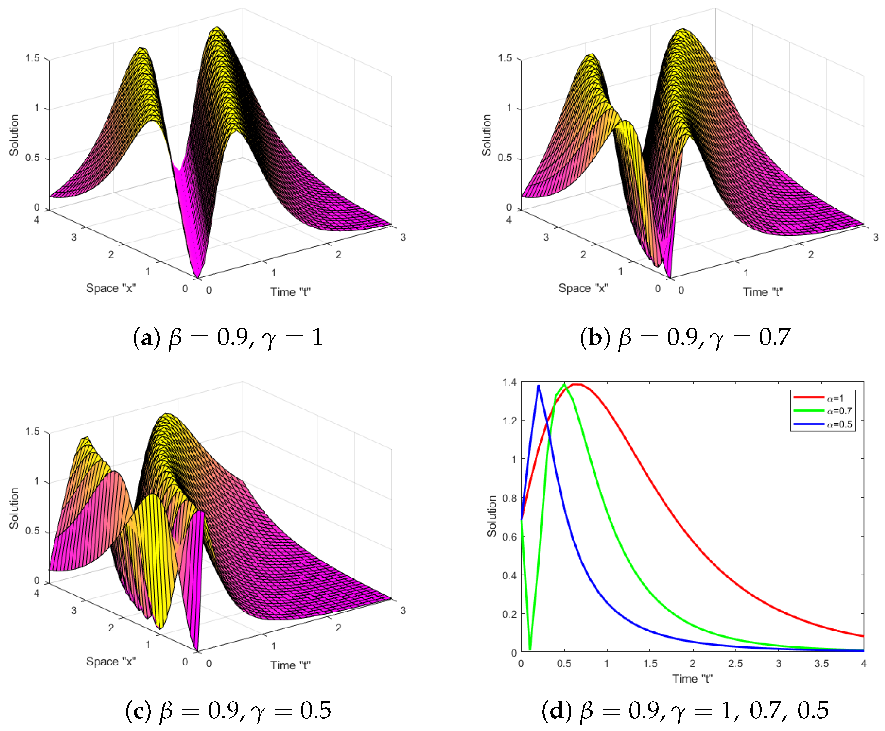
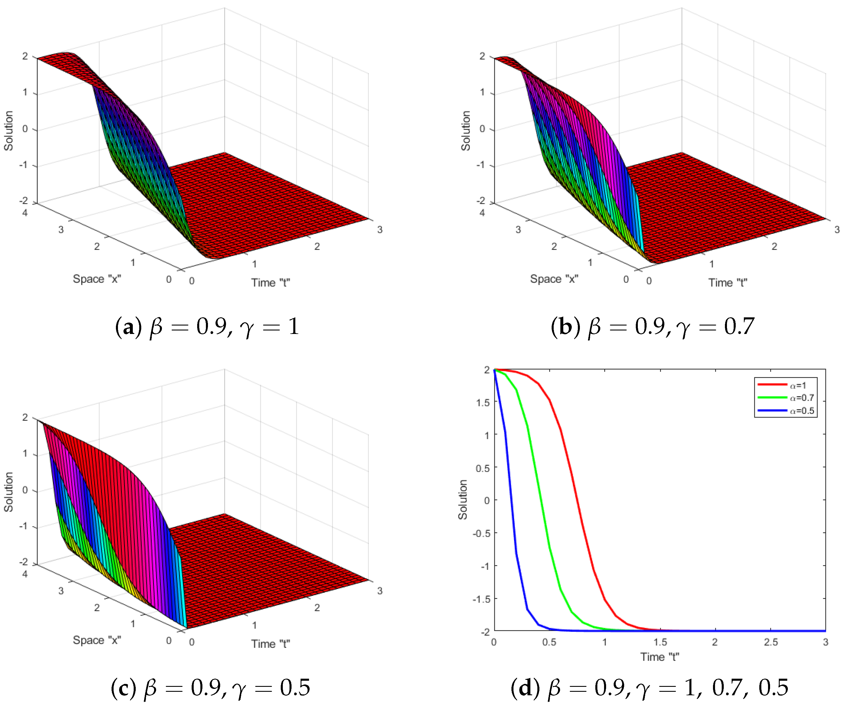
For various solutions described by (10) and (22), we provide 3D and 2D graphs. The graphs analyze the dynamic of the reported solutions based on the fractional values $\gamma$. Firstly, we begin by providing graphs for solution of Equation (10) in Figure 1. We plotted them when ${\mu }_1=1,{\mu }_2=-{\mu }_3=1,{\mu }_4=-2,y=z=1,t\in [0,3]$ and $x\in [0,4],$$\beta =0.9$ and distinct values of $\gamma =1,0.7,0.5$

Secondly, we provide graphs for solution of Equation (22) in Figure 2. We plotted them when ${\mu }_1=1,{\mu }_2=-{\mu }_3=1,{\mu }_4=-2,A_0=a=0,y=z=1,\vartheta =-1,x\in [0,4]$ and $t\in [0,3],$$\beta =0.9,$ and different values of $\gamma =1,0.7,0.5.$

We deduce from previous Figure 1 and Figure 2 that the solution curves do not intersect with one another. In addition, the surface moves into the left when the order of derivative decreases. Therefore, the obtained solutions are novel and can be very useful for understanding physical phenomena.

4. Conclusions

The Boiti–Leon–Manna–Pempinelli equation with a M-truncated derivative (BLMPE-MTD) was investigated. This equation is not studied before with M-truncated derivative. By using the He’s semi-inverse approach and the extended tanh function method, the exact solutions for BLMPE-MTD were obtained. These solutions are essential for making sense of a broad variety of fascinating and challenging physical phenomena. In addition, we generalized some prior results, including those found in [37]. We generated a large number of 2D and 3D diagrams to show how the M-truncated derivative impacts the exact solutions of the BLMPE-MTD. As the order of the derivative decreased, we inferred that the M-truncated derivative caused the surface to shift to the left. In the future work, we can consider BLMPE (1) with stochastic term.

References

- Wang, M.L.; Li, X.Z.; Zhang, J.L. The (G′/G)-expansion method and travelling wave solutions of nonlinear evolution equations in mathematical physics. Phys. Lett. A 2008, 372, 417–423. [Google Scholar] [CrossRef]
- Al-Askar, F.M.; Cesarano, C.; Mohammed, W.W. The analytical solutions of stochastic-fractional Drinfel’d-Sokolov-Wilson equations via (G’/G)-expansion method. Symmetry 2022, 14, 2105. [Google Scholar] [CrossRef]
- Mohammed, W.W.; Al-Askar, F.M.; Cesarano, C. The analytical solutions of the stochastic mKdV equation via the mapping method. Mathematics 2022, 10, 4212. [Google Scholar] [CrossRef]
- Al-Askar, F.M.; Mohammed, W.W. The Analytical Solutions of the Stochastic Fractional RKL Equation via Jacobi Elliptic Function Method. Adv. Math. Phys. 2022, 2022, 1534067. [Google Scholar] [CrossRef]
- Yan, Z.L. Abunbant families of Jacobi elliptic function solutions of the dimensional integrable Davey-Stewartson-type equation via a new method. Chaos Solitons Fractals 2003, 18, 299–309. [Google Scholar] [CrossRef]
- Raheela, M.; Zafar, A.; Bekir, A.; Tariq, K.U. Exact wave solutions and obliqueness of truncated M-fractional Heisenberg ferromagnetic spin chain model through two analytical techniques. Waves Random Complex Media 2023, 1–19. [Google Scholar] [CrossRef]
- He, J.H.; Wu, X.H. Exp-function method for nonlinear wave equations. Chaos Solitons Fractals 2006, 30, 700–708. [Google Scholar] [CrossRef]
- Iftikhar, A.; Ghafoor, A.; Zubair, T.; Firdous, S.; Mohyud-Din, S.T. (G′/G, 1/G)-expansion method for traveling wave solutions of (2 + 1) dimensional generalized KdV, Sin Gordon and Landau-Ginzburg-Higgs Equations. Sci. Res. Essays 2013, 8, 1349–1359. [Google Scholar]
- Khan, K.; Akbar, M.A. The exp(-ϕ(ς))-expansion method for finding travelling wave solutions of Vakhnenko-Parkes equation. Int. J. Dyn. Syst. Differ. Equ. 2014, 5, 72–83. [Google Scholar]
- Seadawy, A.R.; Manafian, J. New soliton solution to the longitudinal wave equation in a magneto-electro-elastic circular rod. Res. Phys. 2018, 8, 1158–1167. [Google Scholar] [CrossRef]
- Mohammed, W.W.; Alshammari, M.; Cesarano, C.; El-Morshedy, M. Brownian Motion Effects on the Stabilization of Stochastic Solutions to Fractional Diffusion Equations with Polynomials. Mathematics 2022, 10, 1458. [Google Scholar] [CrossRef]
- Malfliet, W.; Hereman, W. The tanh method. I. Exact solutions of nonlinear evolution and wave equations. Phys. Scr. 1996, 54, 563–568. [Google Scholar] [CrossRef]
- Al-Askar, F.M.; Cesarano, C.; Mohammed, W.W. The Influence of White Noise and the Beta Derivative on the Solutions of the BBM Equation. Axioms 2023, 12, 447. [Google Scholar] [CrossRef]
- Shah, N.A.; Alyousef, H.A.; El-Tantawy, S.A.; Shah, R.; Chung, J.D. Analytical Investigation of Fractional-Order Korteweg–De-Vries-Type Equations under Atangana–Baleanu–Caputo Operator: Modeling Nonlinear Waves in a Plasma and Fluid. Symmetry 2022, 14, 739. [Google Scholar] [CrossRef]
- Mohammed, W.W.; Al-Askar, F.M.; Cesarano, C.; Aly, E.S. The Soliton Solutions of the Stochastic Shallow Water Wave Equations in the Sense of Beta-Derivative. Mathematics 2023, 11, 1338. [Google Scholar] [CrossRef]
- Katugampola, U.N. New approach to a generalized fractional integral. Appl. Math. Comput. 2011, 218, 860–865. [Google Scholar] [CrossRef]
- Katugampola, U.N. New approach to generalized fractional derivatives. Bull. Math. Anal. Appl. 2014, 6, 1–15. [Google Scholar]
- Kilbas, A.A.; Srivastava, H.M.; Trujillo, J.J. Theory and Applications of Fractional Differential Equations; Elsevier: Amsterdam, The Netherlands, 2016. [Google Scholar]
- Samko, S.G.; Kilbas, A.A.; Marichev, O.I. Fractional Integrals and Derivatives, theory and Applications; Gordon and Breach: Yverdon, Switzerland, 1993. [Google Scholar]
- Sousa, J.V.; de Oliveira, E.C. A new truncated M fractional derivative type unifying some fractional derivative types with classical properties. Int. J. Anal. Appl. 2018, 16, 83–96. [Google Scholar]
- Yusuf, A.; Inc, M.; Baleanu, D. Optical Solitons With M-Truncated and Beta Derivatives in Nonlinear Optics. Front. Phys. 2019, 7, 126. [Google Scholar] [CrossRef]
- Mohammed, W.W.; El-Morshedy, M.; Moumen, A.; Ali, E.E.; Benaissa, M.; Abouelregal, A.E. Effects of M-Truncated Derivative and Multiplicative Noise on the Exact Solutions of the Breaking Soliton Equation. Symmetry 2023, 15, 288. [Google Scholar] [CrossRef]
- Mohammed, W.W.; Al-Askar, F.M.; Cesarano, C. Solutions to the (4+ 1)-Dimensional Time-Fractional Fokas Equation with M-Truncated Derivative. Mathematics 2022, 11, 194. [Google Scholar] [CrossRef]
- Hussain, A.; Jhangeer, A.; Abbas, N.; Khan, I.; Sherif, E.M. Optical solitons of fractional complex Ginzburg–Landau equation with conformable, beta, and M-truncated derivatives: A comparative study. Adv. Differ. Equ. 2020, 612, 2020. [Google Scholar] [CrossRef]
- Yusuf, A.; Sulaiman, T.A.; Mirzazadeh, M.; Hosseini, K. M-truncated optical solitons to a nonlinear Schrödinger equation describing the pulse propagation through a two-mode optical fiber. Opt. Quant. Electron. 2021, 53, 558. [Google Scholar] [CrossRef]
- Wazwaz, A.M. Painleve analysis for new (3 + 1)-dimensional Boiti–Leon–Manna–Pempinelli equations with constant and time-dependent coefficients. Int. J. Numer. Methods Heat Fluid Flow 2019, 30, 4259–4266. [Google Scholar] [CrossRef]
- Darvishi, M.T.; Najafi, M.; Kavitha, L.; Venkatesh, M. Stair and step soliton solutions of the integrable (2 + 1) and (3 + 1)-dimensional Boiti–Leon–Manna–Pempinelli equations. Commun. Theor. Phys. 2012, 58, 785–794. [Google Scholar] [CrossRef]
- Duan, X.; Lu, J. The exact solutions for the (3 + 1)-dimensional Boiti–Leon–Manna–Pempinelli equation. Results Phys. 2021, 21, 103820. [Google Scholar] [CrossRef]
- Osman, M.S.; Wazwaz, A.M. A general bilinear form to generate different wave structures of solitons for a (3 + 1)-dimensional Boiti–Leon–Manna–Pempinelli equation. Math. Methods Appl. Sci. 2019, 42, 6277–6283. [Google Scholar] [CrossRef]
- Liu, J.; Jianqiang, D.; Zeng, Z.; Nie, B. New three-wave solutions for the (3 + 1)-dimensional Boiti–Leon–Manna–Pempinelli equation. Nonlinear Dyn. 2017, 88, 655–661. [Google Scholar] [CrossRef]
- Liu, J.; Tian, Y.; Hu, J. New non-traveling wave solutions for the (3 + 1)-dimensional Boiti–Leon–Manna–Pempinelli equation. Appl. Math. Lett. 2018, 79, 162–168. [Google Scholar] [CrossRef]
- Liu, J. Double-periodic soliton solutions for the (3 + 1)-dimensional Boiti–Leon–Manna–Pempinelli equation in incompressible fluid. Comput. Math. Appl. 2018, 75, 3604–3613. [Google Scholar] [CrossRef]
- Pinar, Z. Analytical studies for the Boiti–Leon–Monna–Pempinelli equations with variable and constant coefficients. Asymptot. Anal. 2019, 4, 1–9. [Google Scholar] [CrossRef]
- Peng, W.; Tian, S.; Zhang, T. Breather waves and rational solutions in the (3 + 1)-dimensional Boiti–Leon–Manna–Pempinelli equation. Comput. Math. Appl. 2019, 77, 715–723. [Google Scholar] [CrossRef]
- Yel, G.; Aktürk, T. A new approach to (3 + 1) dimensional Boiti–Leon–Manna–Pempinelli equation. Appl. Math. Nonlinear Sci. 2020, 5, 309–316. [Google Scholar] [CrossRef]
- Guiqiong, X. Painleve analysis, lump-kink solutions and localized excitation solutions for the (3 + 1)-dimensional Boiti–Leon–Manna–Pempinelli equation. Appl. Math. Lett. 2019, 97, 81–87. [Google Scholar]
- Ali, K.K.; Mehanna, M.S. On some new soliton solutions of (3 + 1)-dimensional Boiti–Leon–Manna–Pempinelli equation using two different methods. Arab J. Basic Appl. Sci. 2021, 28, 234–243. [Google Scholar] [CrossRef]
- Tariq, K.U.; Bekir, A.; Zubair, M. On some new travelling wave structures to the (3 + 1)-dimensional Boiti–Leon–Manna–Pempinelli model. J. Ocean. Eng. Sci. 2022, accepted. [Google Scholar] [CrossRef]
- Raza, N.; Kaplan, M.; Javid, A.; Inc, M. Complexiton and resonant multi-solitons of a (4 + 1)-dimensional Boiti–Leon–Manna–Pempinelli equation. Opt. Quant. Electron. 2022, 54, 95. [Google Scholar] [CrossRef]
- Gencyigit, M.; Senol, M.; Koksal, M.E. Analytical solutions of the fractional (3 + 1)-dimensional Boiti–Leon–Manna–Pempinelli equation. Comput. Methods Differ. Equ. 2023, 1–12. [Google Scholar] [CrossRef]
- He, J.H. Semi-inverse method of establishing generalized variational principles for fluid mechanics with emphasis on turbomachinery aerodynamics. Int. J. Turbo Jet-Engines 1997, 14, 23–28. [Google Scholar] [CrossRef]
- He, J.H. Variational principles for some nonlinear partial differential equations with variable coefficients. Chaos Solitons Fractals 2004, 19, 847–851. [Google Scholar] [CrossRef]
- He, J.H. Some asymptotic methods for strongly nonlinear equations, Internat. J. Mod. Phys. B 2006, 20, 1141–1199. [Google Scholar] [CrossRef]
- Ye, Y.H.; Mo, L.F. He’s variational method for the Benjamin–Bona–Mahony equation and the Kawahara equation. Comput. Math. Appl. 2009, 58, 2420–2422. [Google Scholar] [CrossRef]
- Zahran, E.H.M.; Khater, M.M.A. The modified extended tanh-function method and its applications to the Bogoyavlenskii equation. Appl. Math. Model. 2016, 40, 1769–1775. [Google Scholar] [CrossRef]
Figure 1.
(a–c) indicate 3D-graph of Equation (10) (d) denotes 2D-graph of Equation (10) for distinct values .
Disclaimer/Publisher’s Note: The statements, opinions and data contained in all publications are solely those of the individual author(s) and contributor(s) and not of MDPI and/or the editor(s). MDPI and/or the editor(s) disclaim responsibility for any injury to people or property resulting from any ideas, methods, instructions or products referred to in the content. |
© 2023 by the authors. Licensee MDPI, Basel, Switzerland. This article is an open access article distributed under the terms and conditions of the Creative Commons Attribution (CC BY) license (https://creativecommons.org/licenses/by/4.0/).
Share and Cite
MDPI and ACS Style
Al-Askar, F.M.; Cesarano, C.; Mohammed, W.W. Abundant Solitary Wave Solutions for the Boiti–Leon–Manna–Pempinelli Equation with M-Truncated Derivative. Axioms 2023, 12, 466. https://0-doi-org.brum.beds.ac.uk/10.3390/axioms12050466
AMA Style
Al-Askar FM, Cesarano C, Mohammed WW. Abundant Solitary Wave Solutions for the Boiti–Leon–Manna–Pempinelli Equation with M-Truncated Derivative. Axioms. 2023; 12(5):466. https://0-doi-org.brum.beds.ac.uk/10.3390/axioms12050466
Chicago/Turabian StyleAl-Askar, Farah M., Clemente Cesarano, and Wael W. Mohammed. 2023. "Abundant Solitary Wave Solutions for the Boiti–Leon–Manna–Pempinelli Equation with M-Truncated Derivative" Axioms 12, no. 5: 466. https://0-doi-org.brum.beds.ac.uk/10.3390/axioms12050466
Note that from the first issue of 2016, this journal uses article numbers instead of page numbers. See further details here.