
Review of Quaternion Differential Equations: Historical Development, Applications, and Future Direction


1
Department of Mathematics, Faculty of Mathematics and Natural Sciences, Universitas Padjadjaran, Sumedang 45363, Indonesia
2
Faculty of Science and Natural Resources, Universiti Malaysia Sabah, Kota Kinabalu 88400, Malaysia
*
Author to whom correspondence should be addressed.
Axioms 2023, 12(5), 483; https://0-doi-org.brum.beds.ac.uk/10.3390/axioms12050483
Submission received: 15 December 2022
/
Revised: 27 April 2023
/
Accepted: 12 May 2023
/
Published: 16 May 2023
(This article belongs to the Special Issue Differential Equations and Related Topics)
Abstract
:Quaternion is a four-dimensional and an extension of the complex number system. It is often viewed from various fields, such as analysis, algebra, and geometry. Several applications of quaternions are related to an object’s rotation and motion in three-dimensional space in the form of a differential equation. In this paper, we do a systematic literature review on the development of quaternion differential equations. We utilize PRISMA (preferred reporting items for systematic review and meta-analyses) framework in the review process as well as content analysis. The expected result is a state-of-the-art and the gap of concepts or problems that still need to develop or answer. It was concluded that there are still some opportunities to develop a quaternion differential equation using a quaternion function domain.
1. Introduction
Quaternion is a four-dimensional number system invented by Sir William Rowan Hamilton in 1843 and is also an extension of the complex number system [1]. The quaternion’s structure is similar to complex numbers, which consist of one real and three imaginary parts. Hamilton’s motivation for developing the quaternion emerged while studying complex numbers, which are defined as ordered pairs of two real numbers. These ordered pairs further represent directed line segments in the Cartesian plane. In this representation, the imaginary number i is considered the rotation operator of the directed line segment in the plane. Therefore, this complex number becomes a system that is very suitable for studying directed line segments and rotations in planes.
Hamilton designed a number system that is analogous to the complex number system in order to apply directed and rotational line segments in three-dimensional space. Based on the fact that it is possible to represent complex numbers with ordered pairs of real numbers, it seems natural for Hamilton to use a number system analogy to study directed line segments and rotations in space requiring an ordered triple representation of real numbers. This implies that the numbers are of the form , where a, b, and c are real numbers, while i and j are the imaginaries. Hamilton found faced extreme difficulties in determining a satisfactory multiplication operation on this ordered triplet for several years. This difficulty was explained when the algebraist Frobenius proved that no number aside from an ordinary complex number was able to satisfy all the postulates of ordinary algebra. This caused Hamilton to realize that a number consisting of one real and two imaginary parts were insufficient for the number system required. Hamilton, therefore, needed a number system that consists of one real and three imaginary parts, known as quaternion [2].
Quaternions can be studied from various aspects such as algebra, analysis, and geometry. Structurally, a quaternion is not a commutative ring, hence, it is viewed in terms of matrix and group theory [3]. Several studies on the Fibonacci sequence from the perspective of number theory include [4,5,6,7,8,9], while Karmano (2013) [10] examined the Riemann Zeta quaternion function. Studies on quaternions can also be viewed from the transformation perspective, one of which is the quaternion Fourier transformation [11,12,13,14,15,16]. From the analytical aspect, [17,18] investigated quaternions based on function differentiation, derivatives [19], Hilbert space [20], as well as boundary problems and integrals [21]. An important idea in quaternion is the unit quaternion, it can be represented in special groups, such as the special orthogonal group (SO(3)) and special unitary group (SU(2)) [22,23].
Quaternion was first applied by Oliver Heaviside to physics problems, known as Maxwell’s theory of electromagnetic waves [1]. Since this period, there has been continuous development in the applications of quaternions, such as in the fields of DNA nucleotide patterns, bio-logging, which involves tracking animal and human movements, eye tracking, color processing, signaling, digital image, quantum physics, aerospace, social/economic exchange systems, computer graphics, animation, robotics, and music [24]. It was observed that quaternion is a very efficient tool for analyzing an object’s motion, such as rotation in three-dimensional space. In simple terms, its geometric meaning is the axis and angle of rotation. quaternion is broadly applicable in the fields of animation, kinematics, robotics, etc. [25]. Ken Shoemake in a study, Animating Rotation with Quaternion Curve, popularized the quaternion in computer graphics and introduced spherical linear interpolation (SLERP), which is the optimal interpolation curve between two rotations. It is important to note that quaternions are generally applied in animation for interpolating curves [26]. However, the rotation with a matrix is used when many points have to be transformed, an example is the skin vertices of an animated model, in which Shoemake introduced the conversion between quaternions and matrices in computer graphics. Quaternion, therefore, became a standard topic considered in the higher analysis of computer graphics, control theory, signal processing, such as filtering, orbital mechanics, etc., basically for representing the rotations and orientations in 3D space [27].
Further applications in physics have been performed by [28], using mathematical models of motion, namely rigid posture control, such as movement in space and mechanical robotic arms [29]. Meanwhile, in the kinematics field, the concepts and formulas related to quaternions and rotation in 3D space, as well as their use in error state Kalman filters were developed [30]. The result produced a lot of intuition and geometric interpretation for mechanisms in 3D rotation. Quaternions are also applied in digital signal and image processing using quaternion Fourier transformations. In image processing, the Fourier transform is performed to change the image from spatial into the frequency domain. This is for simplicity as the filtering in the frequency domain is simpler than that of the spatial [31]. When the image on multidimensional numbers (hypercomplex) is implemented, quaternion Fourier transformation is used in color images, specifically the RGB color model, namely red, green, and blue. The three imaginary parts of the quaternion represent the colors red, green, and blue [15], while the quaternion Fourier transformation was continually developed as (1) the quaternion field [13], (2) the uncertainty principle [12], and (3) the use of signals for higher dimensions, such as octonions [14].
The quaternion from the analytical aspect has been studied [17,32] and the function was defined using the concept of left and right derivatives. Furthermore, the analytical concept of complex numbers was developed with regular functions on quaternion. The study by [33] complemented several approaches, such as convergence, trigonometric function, and logarithm, while [34] examined some of the quaternion-valued properties by analogizing complex value functions. In addition, Dzagnize in [18] defined the derivatives in quaternion-valued functions by expanding the holomorphic theory of complex values. Dzagnidze also described the derivative of the quaternion value function using two series of quaternion numbers. This was further complemented by proving the derivatives of several elementary functions with quaternion values, such as polynomial, exponential, trigonometry, and quaternion logarithms [18]. In 2018, Dzagnidze completed the criteria for the requirements and conditions needed for sufficient quaternion functions to be differentiable [35].
It is important to note that the quaternion differential equation is an extension of the ordinary differential equation containing the quaternion value function and its derivatives. The main problem of differential equations is to determine their solution. In [36], real matrix representation was used to solve and prove the existence and uniqueness of homogeneous quaternion differential equations. Furthermore, Campos and Mawhim demonstrated the existence of periodic solutions to quaternion differential equations [37], while Wilczynski provided some sufficient conditions for periodic solutions of the Riccati quaternion differential equations [38]. Riccati’s three-dimensional quaternion differential equations were performed by [39], while Grigorian (2019) found the general solution criteria for the equations [40]. The basic linear quaternion differential equation theory and its application to quantum mechanics, fluid mechanics, Frenet frames in differential geometry, dynamic modeling [41], Kalman filters, etc., are systematically presented by [42]. Moreover, Kou et al (2019) found that the solution of the linear quaternion differential equation has many eigenvalues. Some of the methods already used in solving linear quaternion differential equations include the fundamental matrices [43], Laplace Transformation [44], and Adomian Decomposition Method [45].
In this article, a review of quaternion differential equations using PRISMA (preferred reporting items for systematic review and meta-analyses) framework together with the publish or perish (PoP) program was carried out and the bibliometric mapping was analyzed with VOSviewer. The process for obtaining data and the complete search strategy are presented in Section 2.2, while the result of this systematic literature review is state of the art presented in Section 3.3. In brief, the research GAP obtained is the development of an ordinary differential equation in the real domain (domain of the solution function is real) to a quaternion differential equation with the domain of the solution function is quaternion (ordinary differential equation in the quaternion domain).
2. Materials and Methods
2.1. Basic Concepts of Quaternion
2.1.1. Quaternion
The set of all Quaternion numbers is denoted by If , , , and , then can be written as
represents the scalar or real part, while is the vector or imaginary part.
Suppose where and .
The quaternion addition and multiplication operations are defined as
with
The conjugate from is written as and it is defined as follows:
The functions defined by are called norm of q.
Proposition 1.
The function is defined as follows
This is called an inner product of p and q. The norm of q is written as .
The sets of all quaternion numbers is written as indicate the identity element of quaternion multiplication operations.
If , then there exist such that .
Furthermore,
If , then q is called unit quaternion. The set of all unit quaternion is notated as .
For , there exist and such that .
If then and
Assuming , , , and ). The logarithm function is defined as follows:
If , , and , then the exponent function is defined as
If and , then and .
If , , and , then and
The notation of quaternion is also represented in the form of the Euler formula, Cayley-Dickson, a matrix over real numbers ( matrix), and a matrix over complex numbers ( matrix) [15,30]. The equations are presented in a row below.
where
is the modulus of q.
is the axis of q
is the argument of q,
, and
In this form , is a complex conjugate of .
is denoted in the form of matrix of real numbers , with
and matrix of complex numbers :
2.1.2. Derivative of Quaternion Function
Before the presentation of the quaternion derivatives, the holomorphic functions were discussed in complex value functions. The three methods for building these functions on complex value functions include derivative, polynomial, and gradient [18]. It was discovered that not all quaternion-valued functions are directly applicable to these methods. For example, the derivative only applies to linear functions with real number coefficients and the polynomial method uses the Hausdorff formula and the Cauchy–Riemann equation, while the gradient method utilizes the regular functions and gradient operators.
The derivative method employed the concept of limit for derivative functions, indicating that the functions of quaternion value can have two derivative definitions, due to the non-commutative of the quaternion. Suppose is a function of quaternion value, it means the comparison , are irreplaceable with or . This led to the idea of defining the right derivative as,
and left derivatives as
Polynomial method, suppose polynomial with , and complex coefficient . By replacing by and by , the polynomial is obtained as from complex variables and . . This is a polynomial with a complex variable z; hence, the necessary and sufficient conditions of the Cauchy–Riemann are met.
The gradient method, being the extension of holomorphic function theory in Quaternion was proposed by Futer in 1935 [18], using the properties of regular functions. The Quaternion functions with , is called right-regular, if
and it is turned left-regular, if
Meanwhile, it is known as regular, when it is right-regular, indicating that every regular function is harmonic.
This is called a Laplace’s equation.
Dzagnidze (2018) [35] defined the derivative of the Quaternion function as where , and are the real-value functions for called
Definition 1.
[35]: A Quaternion function , where defined in some neighborhood as of a point is said to be -differentiable at When there exist two quaternion sequences
and such that is finite, the increment of the function can be represented as follows:
where
and
. In this case, the quaternion is called -derivative of the function f at a point and is denoted by . Thus
In the sequel, the symbol represents any function , which satisfies .
Proposition 2.
- (a)
- , for
- (b)
- (c)
- (d)
- .
Furthermore, Dzagnidze also proved several properties, such as linearity of derivative functions, derivatives of composition functions, derivatives of logarithmic functions, necessary and sufficient conditions for derivatives of quaternion functions, etc.
Quaternion derivatives are discussed by Dennis Morris (2016) [47] from the perspective of non-commutative differentiation (structural quaternions are non-commutative divisions algebra) [48]. Differentiation takes the ratio of an infinitesimal amount of one variable and an infinitesimal amount of another variable, . Such a ratio is effectively a product of and . Since quaternions are multiplicatively non-commutative, there is a difference between quaternion versions of and .
Let represent a potential quaternion written as:
Defined the quaternion differentiation operator in the as
with notation only.
To differentiate on the left, we simply matrix multiply this differential operator on the left on the quaternion potential with the understanding that . We have the left defferential:
This gives ( is the matrix element of to the m-th row and n-th column):
Since differentiation is a linear operator; hence, we have:
With the same way, to differentiate on the right, we simply matrix multiply this differential operator on the right on the quaternion potential with the understanding that . We have the right differential:
This gives ( is an element matrix to the m-th row and n-th column):
and
It’s clear that .
2.1.3. Quaternionic Regular Function
In this section, we will discuss the elementary properties of the quaternion regular function (refer to [49,50]). In general regular functions are those which take up the kernel of a proper differential operator in Clifford Algebra (Quaternion is a special type from Clifford algebra [49]).
Definition 2.
The operator
Which acts on the space , where is called Dirac operator and is the m-th partial derivative and
Definition 3.
The operator
Which acts on the space , with is called Cauchy–Fueter Dirac operator where and
Definition 4.
Let
. A function
is called left quaternion regular (right quaternion regular) if and only if
A function which is both left and right quaternion regular is called two-sided quaternion regular. Functions which fulfill the condition
Are called left (right) quaternionic holomorphic.
Let is basis of . The Dirac operator has a form
Together with , it follows that
where , , .
For we get in an analogous way.
The Cauchy–Fueter operator has the corresponding representation
Definition 5.
Let be
defined by
This operator is called adjoint Cauchy–Fueter operator. The operator
defined by
Is called an adjoint Dirac operator.
2.1.4. Quaternion Differential Equation
The quaternion differential equation is an extension of the ordinary differential equation. It is important to note that the fundamental difference between an ordinary and a quaternion differential equation lies in the structural form of the solution. The quaternion’s non-commutative nature showed that the set of all solutions to the quaternion differential equation is in the form of a module, not a vector space [42].
Kou and Xia (2018) [42] provided several forms of quaternion differential equations in terms of mathematical models derived from quaternion applications in several fields, which include quaternion frenet frame in differential geometry, quaternion differential equations in kinematic modeling and attitude dynamics, quaternion differential equations in fluid mechanics and quaternion differential equations in quantum mechanics.
- Quaternion frenet frame on differential geometry.
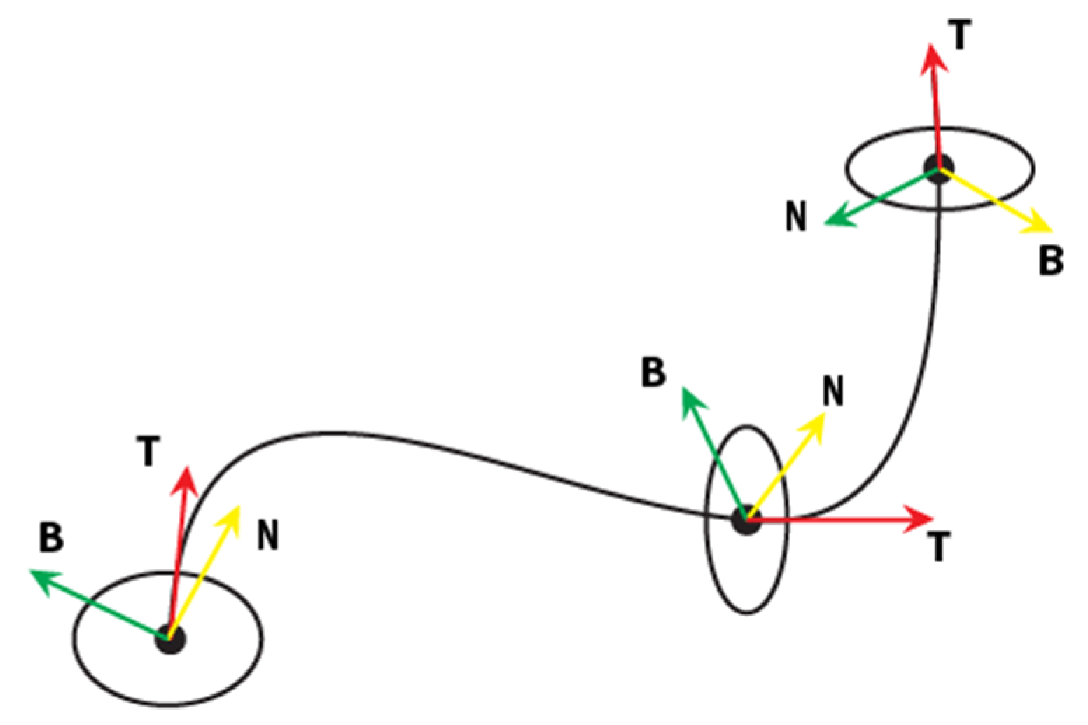
The vector is a function of s and the tangent vector is defined on every . It was found that the coordinate system of the frenet frame consists of a tangent vector , a binormal vector , and a principal normal vector , as shown in Figure 1.
The global position system (GPS) used for guidance and navigation produces orientation measurements where the equation of motion in fours assumes a very small degree of rotation in a very small time t, expressed as
The frenet frame configuration satisfies the following differential equation:
where, is the scalar quantity of the derivative of the curve. The curvature of the curve and the torque is expressed as
This shows that all 3D coordinates of the frame can be expressed in terms of quaternions. If
then the first-order quaternion differential equation can be written as,
where
- b.
- Quaternion differential equations in kinematic modeling and attitude dynamics.
The GPS used for guidance and navigation produced orientation measurement when the motion in a quaternion assumed a very small degree of rotation in a very small time t, expressed as
where with the quaternion derivation approach
and is the angular velocity rotation.
- c.
- Quaternion differential equations in fluid mechanics.
The three-dimensional Euler equation has a Riccati quaternion structure,
where and are a 4-vector, represents a scalar, denotes a 3-vector, and is defined as the Hessian matrix P.
- d.
- Quaternion differential equations in quantum mechanics.
The standard formula for nonrelativity quantum mechanics is the complex wave function that was affected by the real potential , satifying the Schrodinger equation
The generalization of classical quantum mechanics to quaternion was performed using the operators.
This is generalized to the complex potential in order to obtain
When is a quaternion wave function, then the equation obtained is as follows:
The Schrodinger equation is therefore written as
This form is a partial differential equation that can be reduced by using the separate variable method
to the second-order Quaternion differential equation
2.2. Database and Search Strategy
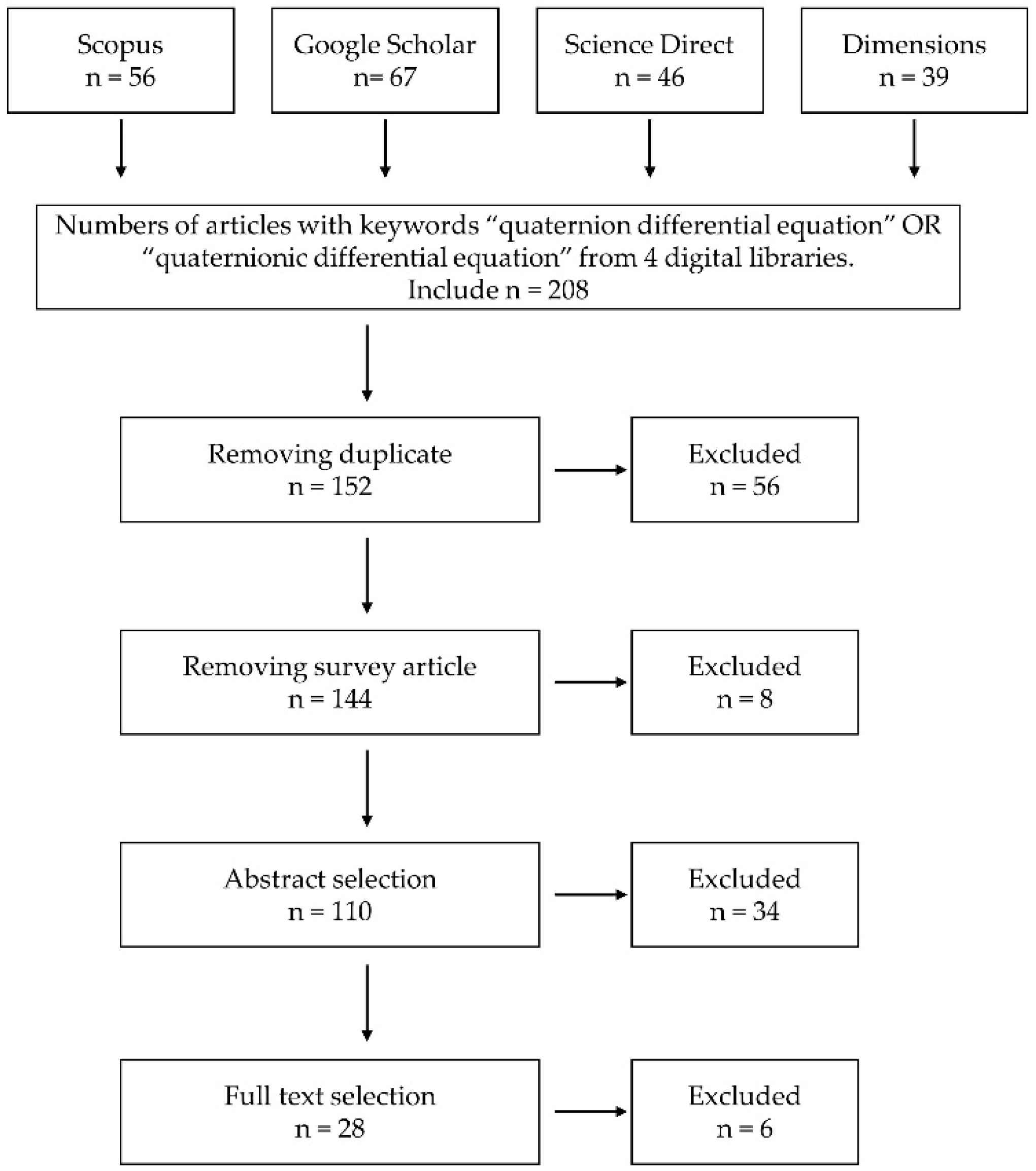
This section describes how to obtain literature data. The procedures performed include searching, filtering, and selecting data. Firstly, it begins by searching for literature from four scientific article databases, namely Scopus, Science Direct, Dimensions, and Google Scholar. The keywords used are “quaternion differential equation” and “quaternionic differential equation” with data from 2000 to 2022. The search strategy for data mining from Google Scholar and Scopus uses the Publish or Perish (PoP) 7.0 application while in the Science Direct database and Dimensions, directly using the websites (http://www.science.direct.com accessed on 19 January 2023 and http://www.dimensions.com accessed on 19 January 2023. Data from Google Scholar obtained 68 articles, Scopus 57 articles, Science Direct 47 articles, and Dimensions 38 articles. Details are presented in the following Table 1.
Next, the paper that was selected from the four digital libraries in the following way: first, a duplicate data check was carried out, in this paper the Scopus database was used as a reference, that is, if one paper is found in two or more databases, for example, paper “x” is on Google Scholar and Scopus, then what is entered is paper “x” in Scopus, while the one in Google Scholar is deleted, this also applies to Science Direct and Dimensions. Checking for duplicate papers is done by exporting and combining all data into MS Excel 2013 and filtering if duplicates are based on the title. After checking for duplicative data, the number of unique data was 152 papers.
The next stage is the manual selection stage, namely by filtering papers with the type of review articles or surveys. Only papers with the type of scientific journal publications are entered, the result is a total of 144 papers (namely Datasets_1). This Datasets_1 will be used as material in conducting an analysis using VOSviewer. Of the 144 papers, the next process is selecting papers through abstracts, meaning removing papers irrelevant to this research. After the abstract selection process, 110 paper data were obtained. The final step is to select papers by reading the full text, then 28 papers are obtained. This data is used as study material in this study. In general, the steps for filtering data are shown in the following Figure 2.
2.3. Data Analysis and Visualization
The Microsoft Excel 2013 application program was used to analyze the data, while VOSviewer 1.6.14 application program was considered for the visualization. We performed a bibliometric analysis for datasets using VOSviewer for mapping. This analysis technique is often used for literature analyses intent on obtaining bibliographic overviews of scientific selections of highly cited publications [51]. It can recover a list of author productions, national or subject bibliographies, or other specialized subject patterns the indicators utilized include publication statistics, co-authoring, the collaboration of authors, institutions, countries, impact factors, citations, etc. In analyzing bibliometric mapping, the PoP 7.0 application program was employed, while the VOSviewer program was used for visualization.
3. Results
3.1. Result from Bibliometric Analysis
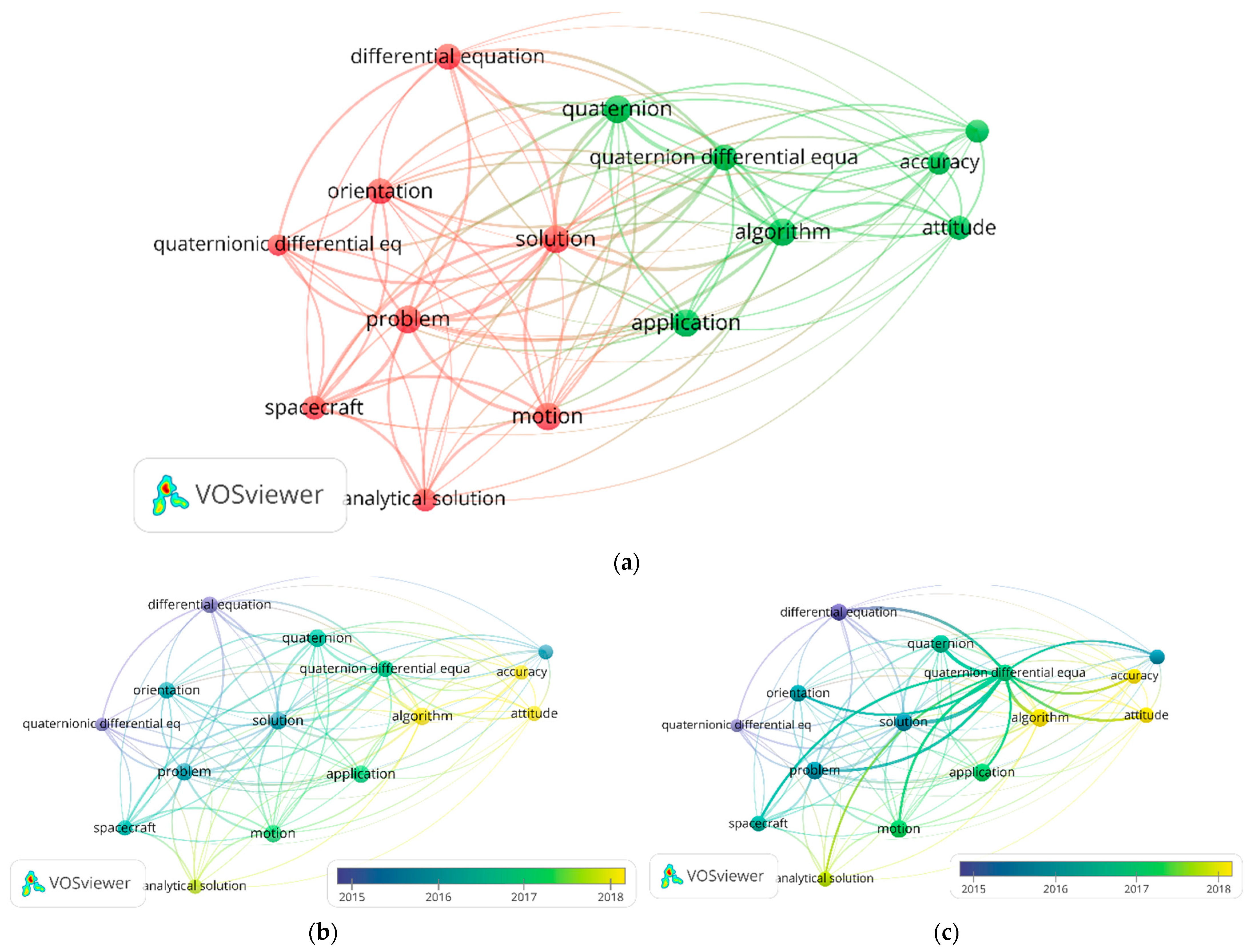
In conducting a co-occurrence analysis of Datasets_1, we searched for the most frequently occurring words from all documents. Datasets_1 contains data taken based on the title, abstract, and keywords only. VOSviewer has a supporting feature that allows us to evaluate co-occurrence keyword relationships from the menu in VOSviewer. The minimum number of word occurrences in this document is seven, meaning that a word will appear if the word is found in seven articles or more. VoSviewer provides 15 items which are divided into 2 clusters, red clusters consist of 8 items, and green clusters (7 items) as shown in Figure 3a.
The keyword quaternion differential equation is in the green cluster, while the keyword quaternion differential equation is in the red cluster. Referring to the overlay visualization (Figure 3b), the term, “quaternionic differential equation” was widely used before 2014 or 2015, whereas since 2016–2017 researchers have often used the term “quaternion differential equation”.
Based on Figure 3c, research trends related to the quaternion differential equation in the last 10 years include problem, solution, orientation, spacecraft, strap-down inertial navigation, motion, analytical solution, accuracy, attitude, and algorithm.
3.2. Development of Quaternion Differential Equation
An important role in different branches of mathematical analysis is differential equations. Its conception will that of differential and integral calculus. In the seventeenth century, Sir Isaac Newton found firstly the solution to differential equations with the help of an infinite series. The article on this subject was published firstly by Gottfried Wilhelm von Leibniz (1646–1716) [52]. The development of differential equations progresses very quickly. Scientists keep developing differential equations, such as in theory, applications, and methods to find the solutions.
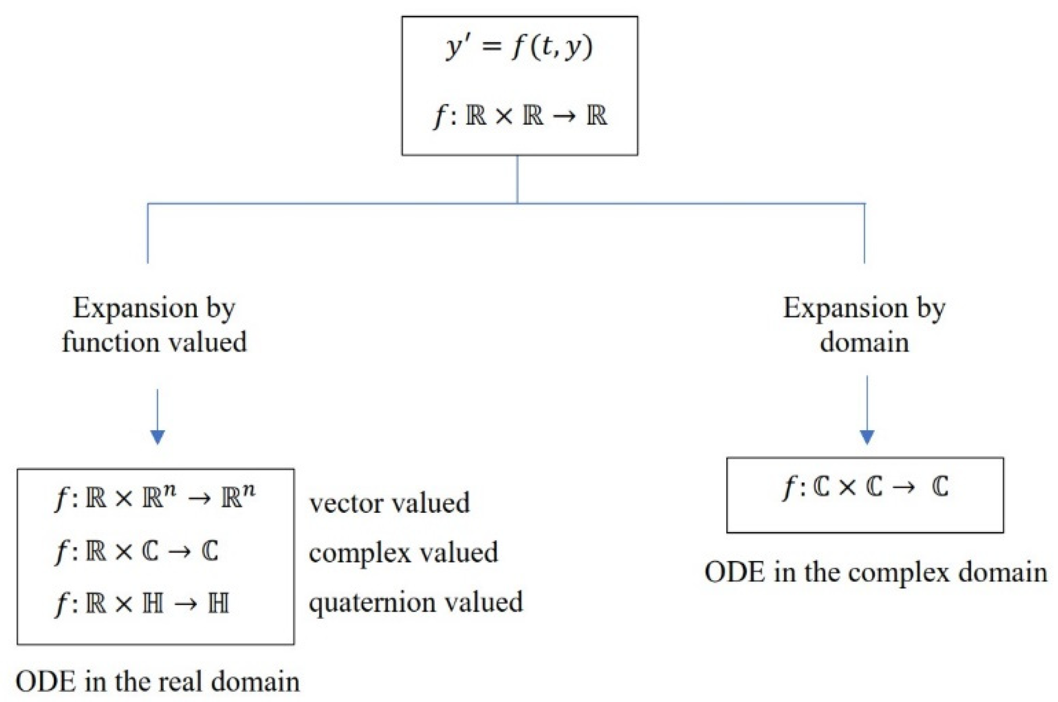
A differential equation is an equation involving an unknown function and its derivatives. A differential equation is an equation involving an unknown function, its derivatives, and eventual known quantities, if an unknown function has only one independent variable, it is called an ordinary differential equation (ODE). The first order ODE is written:
where is the independent variable, is the dependent variable (is the unknown function), with , and with open [53].
The development of the ODE to quaternion differential equations concept [54] is carried out in the following steps: (i) the real-valued functions with , is expanded to quaternion-valued functions with . (ii) the domain of the function , is expanded to , and (iii) the real-valued function is expanded to a quaternion-valued function . So that the explicit form of quaternion differential equations is obtained as:
where is the independent variable, is the dependent variable.
ODE (in the real domain and real-valued function) can be extended both in the domain part and in the function value. In Figure 4, the expansion of ODE based on the function value, including vector-valued, complex-valued [55], quaternion-valued [36,37,38,42,56], Banach space [54], etc. While the extension of ODE based on the domain is from real to complex, which is often said as ODE in the complex domain [57,58,59].
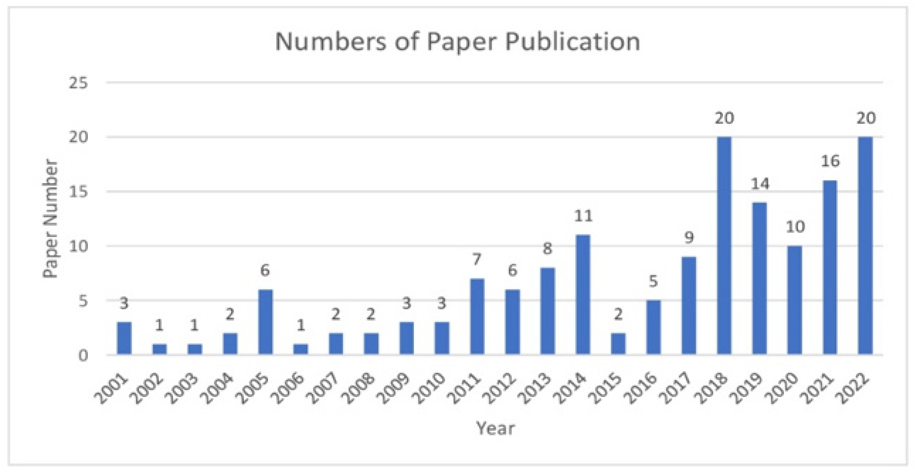
Based on Datasets_1, the number of publications related to quaternion differential equations during the period 2001 to 2022 have fluctuations (up and down), but overall, more than half (53%) are in the last 5 years. In general, it has increased as numbers of publications go up. The highest number was in 2018 and 2022, namely 20 publications each. Full details can be seen in Figure 5. This shows that the research of quaternion differential equations is very important and very interesting to be carried out by researchers.
3.3. Result from Systematic Literature Review
The results of the quaternion from an analytical aspect were presented by Sudbery [17] in the article entitled “Quaternionic Analysis”. Sudbery defined the derivative of a function using the left and right derivative concepts and then developed the analytical concept of functions on complex numbers with regular quaternion. Furthermore, Georgiev et al. [33], in an article entitled “New Aspects on Elementary Functions” in the context of quaternionic analysis, complemented several approaches, including line converge, trigonometric function, and logarithm. Stover [34] examined the various properties of quaternion-valued functions by analogizing complex value functions in an article titled “A Survey of Quaternionic Analysis”.
Dzagnidze [18] explained the derivatives of quaternion-valued functions in a study on the “Differentiability of Quaternion Functions”. Dzagnize expanded the holomorphic theory of complex-valued functions on quaternion value and further defined its derivative, using two rows of quaternions in number. This was complemented by proving the various derivatives of quaternion functions, such as polynomials, exponentials, trigonometry, and logarithms. In 2018, Dzagnidze completed the criteria needed for differentiating the requirements and conditions in the article titled “New Properties of Quaternion Function”.
It is important to reiterate that the quaternion differential equation is an extension of the ordinary differential equation containing quaternion value functions and their derivatives. The main problem of differential equations is the solution and this is the reason Leo and Ducati [36] solved several quaternion differential equations using real matrix representations. Furthermore, they proved the existence and viability of homogeneous quaternion differential equation solutions. Campos and Waphin [37] established the existence of periodic solutions with quaternion differential equations, and Wilczynski [38] provided some sufficient conditions to periodically solve the Riccati quaternion differential equations. The three-dimensional Riccati quaternion differential equation was carried out by Papillon and Tremblay [39], while Grigorian (2019) showed the general solution criteria. The basic theory of linear quaternion differential equations was provided by Kou and Xia [42] in their study on linear quaternion differential equations. In addition, Kou and Xia [42] stated several forms of quaternion differential equations, which include the quaternion frenet frame, kinematic modeling, attitude dynamics, fluid mechanics, and quantum mechanics.
When solving quaternion differential equations of different shapes, it is necessary to select and apply the appropriate method. For example, Kou et al. [43] applied the fundamental matrices to solve linear quaternion differential equation systems, Cai and Kou [44] used Laplace transformation when solving linear quaternion differential equations, and Donachali and Jafari [45] employed the Adomian decomposition method.
According to Table 2. the derivative of the quaternion function in [17,18,33,34,35] is a quaternion, the quaternion differential equations in [36,37,38,40,42,43,44,45] is an equation involving an unknown quaternion-valued function with domain real and its derivatives, while the method in [44,45] is the Laplace transformation and the Adomian decomposition.
4. Discussion
The study of quaternions from the analytical perspective focused more on the properties and characteristics of quaternion-valued functions, both in terms of functional differentiation and their holomorphic properties. It was observed that some definitions of quaternion-valued functions are related to complex values because they are an extension of complex functions. The requirement is that a function with a quaternion value is differentiable at a point when the function is holomorphic. It is also important to note that holomorphic properties are an extension of the analytical properties of complex-valued functions. The Cauchy–Riemann criteria for complex-valued functions were modified for the quaternion value.
The equation containing a quaternion function and its derivatives is called a quaternion differential equation, which is also an extension of an ordinary differential equation. Studies on quaternion differential equations are still limited to quaternion functions in the domain of real numbers. The various forms of this equation that have been examined include linear quaternion differential equation and Riccati differential equation. Furthermore, the methods used to solve quaternion differential equations include the Laplace transform [44] and the Adomian decomposition [45].
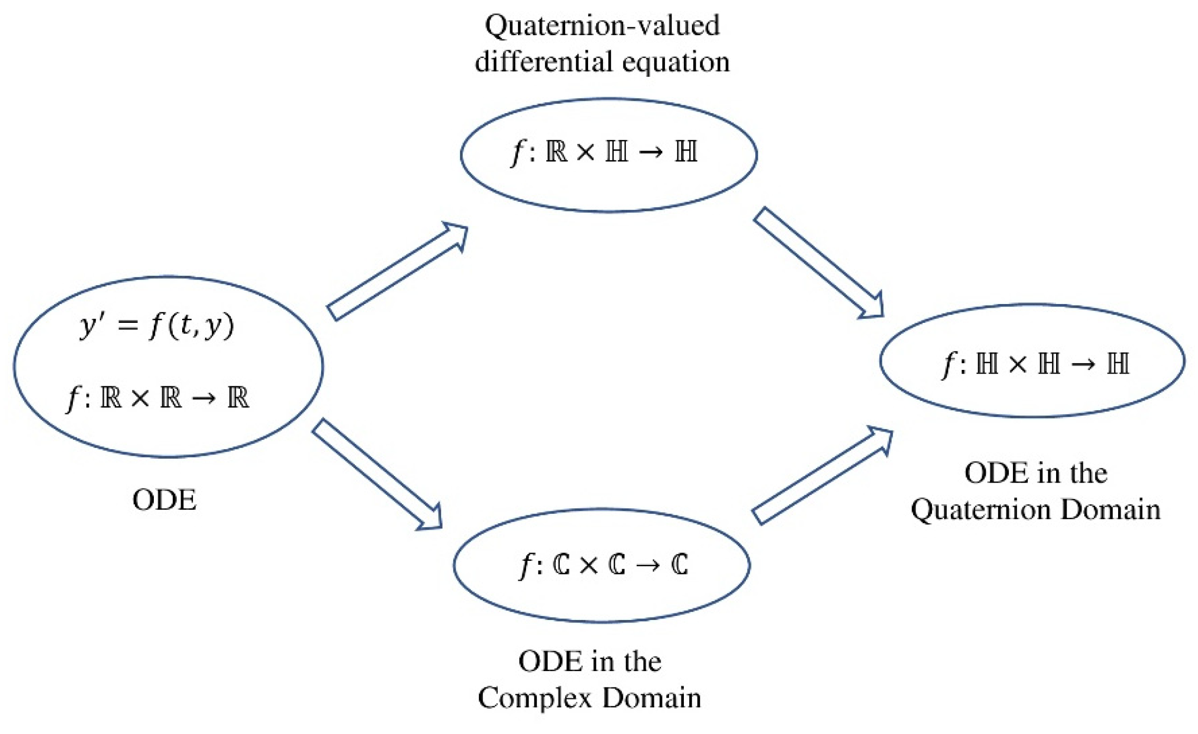
Based on the description above, until now this research on quaternion differential equations only involves quaternion-valued functions (real domain) and their derivatives. The question is, what if this quaternion differential equation contains quaternion-valued functions with quaternion domains and their derivatives? It is very possible, it does mathematically. Given that, to develop a quaternion differential equation with a domain to a quaternion differential equation with a domain, which is the basic premise that quaternion space is an extension of complex space. In the complex space, its differential equation (complex differential equation) [57,58] has been developed from the domain to the domain. By studying the characteristic of complex functions, holomorphicity, differentiation, Cauchy–Riemann criterion, etc., we believe that the development of this extension to a quaternion-valued function can be done. The next question is if the quaternion differential equation development of this kind can be constructed successfully, what is the geometric interpretation? When this kind of quaternion differential equation can be applied? What methods can be used to find the solutions? Of course, this question is very important and interesting to be studied in the future. Figure 6 shows how the route to develop the proposed ODE in the quaternion domain () can be carried out, i.e., either from the ODE with the real domain (quaternion-valued differential equation) in the form of or from ODE in the complex domain in the form
5. Conclusions
In this paper, we showed a systematic literature review of the quaternion differential equation. We screened 208 papers from four digital libraries, namely Google Scholar, Scopus, Science Direct, and Dimensions. After filtering duplicates, titles, and abstracts, 144 articles were obtained (Dataset_1). We performed a bibliometric analysis for Dataset_1, how the usage of the bibliographic mapping technique can reveal an overview of the existing themes as well as the changes over time. This study presents that publications of quaternion differential equations have increased over the last two decades. The description of themes can serve as a basis to study in the future.
Based on the above facts, it was concluded that there are still possibilities for developing a quaternion differential equation with a quaternion function domain and its derivatives. This is based on the differentiability and holomorphism of the quaternion function concept, defined by Sudbery [17], Georgiev et al. [33], Stover [34], Dzagnidze [18,35], and Morris [47,48]. It is therefore believed that this article is useful in finding the future route for the quaternion differential equation development with a quaternion function domain and it is called ordinary differential equation in the quaternion domain.
Author Contributions
Conceptualization, methodology, A.K. and A.K.S.; validation, A.K.S., E.R. and J.S.; formal analysis, investigation, resources, A.K. and A.K.S.; writing—original draft preparation, writing—review and editing, A.K.; supervision, A.K.S., E.R. and J.S.; funding acquisition, A.K. and A.K.S. All authors have read and agreed to the published version of the manuscript.
Funding
This research was funded by Universitas Padjadjaran through the scheme Riset Disertasi Doktor Unpad (RDDU), grant number 1427/UN6.3.1/LT/2020.
Data Availability Statement
Not applicable.
Acknowledgments
The authors wish to thank the Directorate of Research and Community Service (DRPM) of Universitas Padjadjaran. We also would like to thank anonymous referees for their valuable comments and critiques on the previous version of the manuscript.
Conflicts of Interest
The authors declare no conflict of interest.
References
- Familton, J.C. Quaternions: A History of Complex Noncommutative Rotation Groups in Theoretical Physics. Ph.D. Thesis, Columbia University, New York, NY, USA, 2015. [Google Scholar]
- Tait, P.G. An Elementary Treatise Quaternions, 2nd ed.; Nabu Press: Charleston, SC, USA, 1878; ISBN 3663537137. [Google Scholar]
- Voight, J. Quaternion Algebras; Springer Nature: Berlin/Heidelberg, Germany, 2020. [Google Scholar]
- Kaya, O.; Onder, M. On Fibonacci and Lucas Vectors and Quaternions. Univers. J. Appl. Math. 2018, 13, 156–163. [Google Scholar] [CrossRef]
- Catarino, P. A Note on h(x)—Fibonacci Quaternion Polynomials. Chaos Solitons Fractals 2015, 77, 1–5. [Google Scholar] [CrossRef]
- Halici, S. On Fibonacci Quaternions. Adv. Appl. Clifford Algebr. 2012, 22, 321–327. [Google Scholar] [CrossRef]
- Halici, S.; Karataş, A. On a Generalization for Fibonacci Quaternions. Chaos Solitons Fractals 2017, 98, 178–182. [Google Scholar] [CrossRef]
- Horadam, A.F. Complex Fibonacci Numbers and Fibonacci Quaternions. Am. Math. Mon. 2012, 70, 289–291. [Google Scholar] [CrossRef]
- Tan, E.; Yilmaz, S.; Sahin, M. On a New Generalization of Fibonacci Quaternions. Chaos Solitons Fractals 2016, 82, 1–4. [Google Scholar] [CrossRef]
- Kamano, K. Analytic Continuation of the Lucas Zeta and L-Functions. Indag. Math. 2013, 24, 637–646. [Google Scholar] [CrossRef]
- De Bie, H.; De Schepper, N.; Ell, T.A.; Rubrecht, K.; Sangwine, S.J. Connecting Spatial and Frequency Domains for the Quaternion Fourier Transform. Appl. Math. Comput. 2015, 271, 581–593. [Google Scholar] [CrossRef]
- Bahri, M.; Hitzer, E.S.M.; Hayashi, A.; Ashino, R. An Uncertainty Principle for Quaternion Fourier Transform. Comput. Math. Appl. 2008, 56, 2398–2410. [Google Scholar] [CrossRef]
- Hitzer, E.M.S. Quaternion Fourier Transform on Quaternion Fields and Generalizations. Adv. Appl. Clifford Algebr. 2007, 17, 497–517. [Google Scholar] [CrossRef]
- Lian, P. The Octonionic Fourier Transform: Uncertainty Relations and Convolution. Signal Process. 2019, 164, 295–300. [Google Scholar] [CrossRef]
- Ell, T.A.; Le Bihan, N.; Sangwine, S.J. Quaternion Fourier Transforms for Signal; Castanié, F., Ed.; ISTE Ltd.: London, UK, 2014; ISBN 9781848214781. [Google Scholar]
- Bahri, M.; Toaha, S.; Rahim, A.; Ivan, M. On One-Dimensional Quaternion Fourier Transform On One-Dimensional Quaternion Fourier Transform. J. Phys. Conf. Ser. 2019, 1341, 062004. [Google Scholar] [CrossRef]
- Sudbery, A. Quaternionic Analysis; Cambridge University Press: Cambridge, UK, 1979. [Google Scholar] [CrossRef]
- Dzagnidze, O. On the Differentiability of Quaternion Functions. arXiv 2012, arXiv:1203.5619. [Google Scholar] [CrossRef]
- Chudá, H. Universal Approach to Derivation of Quaternion Rotation Formulas. MATEC Web Conf. 2019, 292, 01060. [Google Scholar] [CrossRef]
- Van Leunen, H. Quaternions and Hilbert Spaces. 2015. Available online: https://www.researchgate.net/publication/282655670_Quaternions_and_Hilbert_spaces (accessed on 19 December 2021).
- Ha, V.T.N. Helmholtz Operator in Quaternionic Analysis. Ph.D Dissertation, Freien Universitat, Berlin, Germany, 10 February 2005. [Google Scholar]
- Hashim, H.A. Special Orthogonal Group SO(3), Euler Angles, Angle-axis, Rodriguez Vector and Unit-Quaternion: Overview, Mapping and Challenges. arXiv. 2019. Available online: https://arxiv.org/abs/1909.06669 (accessed on 19 December 2021).
- Sveier, A.; Sjøberg, A.M.; Egeland, O. Applied Runge-Kutta-Munthe-Kaas Integration for the Quaternion Kinematics. J. Guid. Control. Dyn. 2019, 42, 2747–2754. [Google Scholar] [CrossRef]
- Klitzner, H. The Culture of Quaternions The Phoenix Bird of Mathematics; New York Academy of Sciences, Lyceum Society: New York, NY, USA, 1 June 2015. [Google Scholar] [CrossRef]
- Shoemake, K. Animating Rotation with Quaternion Curves. ACM SIGGRAPH Comput. Graph. 1985, 19, 245–254. [Google Scholar] [CrossRef]
- Dam, E.B.; Koch, M.; Lillholm, M. Quaternions, Interpolation and Animation; Institute of Computer Science University of Copenhagen: Denmark, Copenhagen, 1998. [Google Scholar]
- Waldvogel, J. Quaternions for Regularizing Celestial Mechanics—The Right Way. Celest. Mech. Dyn. Astron. 2008, 102, 149–162. [Google Scholar] [CrossRef]
- Kwasniewski, A.K. Glimpses of the Octonions and Quaternions History and Today’ s Applications in Quantum Physics. Adv. Appl. Clifford Algebr. 2012, 22, 87–105. [Google Scholar] [CrossRef]
- Haetinger, C.; Malheiros, M.; Dullius, E.; Kronbauer, M. A Quaternion Application to Control Rotation Movements in The Three Dimensional Space of an Articulate Mechanical Arm Type Robot Built from Low Cost Materials as a Supporting Tool for Teaching at The Undergraduate Level. In Proceedings of the Global Congress on Engineering and Technology Education, São Paulo, Brazil, 13–16 March 2005. [Google Scholar]
- Solà, J. Quaternion Kinematics for The Error-State Kalman Filter. arXiv 2017, arXiv:1711.02508. [Google Scholar]
- Xie, C.; Kumar, B.V.K.V. Quaternion Correlation Filters for Color Face Recognition. In Proceedings of the Security, Steganography, and Watermarking of Multimedia Contents VII, San Jose, CA, USA, 17–20 January 2005; Volume 5681, pp. 486–494. [Google Scholar]
- Giirlebeck, K.; SproBig, W. Quatemionic Analysis and Elliptic Boundary Value Problems; Birkhäuser Basel: Basel, Switzerland, 1990; ISBN 2013206534. [Google Scholar]
- Georgiev, S. New Aspects on Elementary Functions in the Context of Quaternionic Analysis. Cubo 2012, 14, 93–110. [Google Scholar] [CrossRef]
- Stover, C. A Survey of Quaternionic Analysis; Florida State University: Tallahassee, FL, USA, 2014. [Google Scholar] [CrossRef]
- Dzagnidze, O. On Some New Properties of Quaternion Functions. J. Math. Sci. 2018, 235, 557–603. [Google Scholar] [CrossRef]
- De Leo, S.; Ducati, G.C. Solving Simple Quaternionic Differential Equations. J. Math. Phys. 2003, 44, 2224–2233. [Google Scholar] [CrossRef]
- Campos, J.; Mawhin, J. Periodic Solutions of Quaternionic-Valued Ordinary. Ann. Di Mat. 2006, 185, 109–127. [Google Scholar] [CrossRef]
- Wilczynski, P. Quaternionic-Valued Ordinary Differential Equations. Riccati Equ. 2009, 247, 2163–2187. [Google Scholar] [CrossRef]
- Papillon, C.; Tremblay, S. On a Three-Dimensional Riccati Differential Equation and its Symmetries. J. Math. Anal. Appl. 2018, 458, 611–627. [Google Scholar] [CrossRef]
- Grigorian, G.A. Global Solvability Criteria for Quaternionic Riccati Equations. Arch. Math. 2019, 57, 83–99. [Google Scholar] [CrossRef]
- Zhi, W.; Chu, J.; Li, J.; Wang, Y. A Novel Attitude Determination System Aided by Polarization Sensor. Sensors 2018, 10, 158. [Google Scholar] [CrossRef]
- Kou, K.I.; Xia, Y.; Xia, Y.-H. Linear Quaternion Differential Equations: Basic Theory and Fundamental Results. Stud. Appl. Math. 2018, 141, 1–43. [Google Scholar] [CrossRef]
- Kou, K.I.; Liu, W.-K.; Xia, Y.-H. Solve the Linear Quaternion-Valued Differential Equations Having Multiple Eigenvalues. J. Math. Phys. 2019, 60, 023510. [Google Scholar]
- Cai, Z.; Kou, K.L. Laplace Transform: A New Approach in Solving Linear Quaternion Differential Equations. Math. Methods Appl. Sci. 2017, 41, 4033–4048. [Google Scholar] [CrossRef]
- Donachali, A.K.; Jafari, H. A Decomposition Method for Solving Quaternion Differential Equations. Int. J. Appl. Comput. Math. 2020, 123, 1–7. [Google Scholar] [CrossRef]
- Jia, Y.-B. Quaternions. Com S 2019, 477, 577. [Google Scholar]
- Morris, D. Elementary Calculus from an Advanced Standpoint; Abane and Right: Port Mulgrave, UK, 2016. [Google Scholar]
- Morris, D. Quaternions; Abane and Right: Port Mulgrave, UK, 2015. [Google Scholar]
- Gürlebeck, K.; Sprössig, W. Quaternionic and Clifford Calculus for Physicists and Engineers; Willey: Hoboken, NJ, USA, 1998. [Google Scholar]
- Gentili, G.; Stoppato, C.; Struppa, D.C. Regular Functions of a Quaternionic Variable; Springer: Cham, Switzerland, 2022; ISBN 9783031075308. [Google Scholar] [CrossRef]
- Ellegaard, O.; Wallin, J.A. The bibliometric analysis of scholarly production: How great is the impact? Scientometrics 2015, 105, 1809–1831. [Google Scholar] [CrossRef]
- Simmons, G.F. Differential Equations with Applications and Historical Notes, 3rd ed.; Boggess, A., Rosen, K., Eds.; CRC Press: New York, NY, USA, 2017; Volume 4, ISBN 2013206534. [Google Scholar]
- Nagy, G. Ordinary Differential Equations; Michigan State University: East Lansing, MI, USA, 2020. [Google Scholar]
- Deimling, K. Lecture Notes in Mathematics: Ordinary Differential Equations in Banach Spaces; Springer: Berlin/Heidelberg, Germany, 2013; Volume 2084, ISBN 9783319008240. [Google Scholar]
- Yang, B.; Bao, W. Complex-Valued Ordinary Differential Equation Modeling for Time Series Identification. IEEE Access 2019, 7, 41033–41042. [Google Scholar] [CrossRef]
- Feng, Z.; Kit, C.; Kou, I. Solving Quaternion Ordinary Differential Equations with Two-Sided Coefficients. Qual. Theory Dyn. Syst. 2017, 17, 441–462. [Google Scholar] [CrossRef]
- Hille, E. Ordinary Differential Equations in the Complex Domain by Einar Hille (z-lib.org).pdf; John Willey and Sons: San Diego, CA, USA, 1976. [Google Scholar]
- Laine, I. Complex differential equations. In Handbook of Differential Equations: Ordinary Differential Equations; Chapman and Hall/CRC: Boca Raton, FL, USA, 2008; Volume 4, pp. 269–363. ISBN 9780444530318. [Google Scholar] [CrossRef]
- Haraoka, Y. Linear Differential Equations in the Complex Domain: From Classical Theory to Forefront; Springer: Berlin/Heidelberg, Germany, 2020; Volume 2271, ISBN 9783030546625. [Google Scholar] [CrossRef]
Figure 1.
Frenet Frame on a Curve (Modified by [42]).
Figure 1.
Frenet Frame on a Curve (Modified by [42]).

Figure 2.
Diagram of the data selection process.

Figure 3.
(a) Network visualization of co-occurrence word relation in datasets, (b) Overlay visualization in datasets, (c) Overlay visualization in datasets for quaternion differential equation.
Figure 3.
(a) Network visualization of co-occurrence word relation in datasets, (b) Overlay visualization in datasets, (c) Overlay visualization in datasets for quaternion differential equation.

Figure 4.
Development of ordinary differential equations in the existing literature.

Figure 5.
Data for publications of works from 2001 to 2022.

Figure 6.
The route to develop the proposed ODE in the quaternion domain.


Table 1.
Number of publications from four database.
| Keyword | Google Scholar | Scopus | Science Direct | Dimensions |
|---|---|---|---|---|
| “quaternion differential equation” | 55 | 45 | 38 | 27 |
| “quaternionic differential equation” | 13 | 12 | 9 | 11 |
| Total | 68 | 57 | 47 | 38 |
Table 2.
The list of quaternion papers based on topic and object.
| No | Authors | Title | Year | Topic | Object |
|---|---|---|---|---|---|
| 1 | Anthony Sudbery [17] | Quaternionic Analysis | 1978 | function derivative | |
| 2 | S. Georgiev [33] | New Aspects of Elementary Functions in the Context of Quaternionic Analysis | 2012 | quaternion elementary function derivative | |
| 3 | Christopher Stover [34] | A Survey of Quaternionic Analysis | 2014 | derivative/the analytic function | |
| 4 | Omar Dzagnidze [18] | On the Differentiability of Quaternion Functions | 2012 | function derivative | |
| 5 | Omar Dzagnidze [35] | On Some New Properties of Quaternion Function | 2018 | function derivative | |
| 6 | Stefano De Leo and Gisele C. Ducati [36] | Solving simple Quaternionic differential equations | 2003 | quaternion differential equations | |
| 7 | Juan Campos and Jean Mawhin [37] | Periodic solutions of Quaternionic-valued ordinary differential equations | 2005 | quaternion differential equations | |
| 8 | Paweł Wilczynski [38] | Quaternionic-valued ordinary differential equations. The Riccati equation | 2009 | Riccati quaternion differential equation | |
| 9 | Charles Papillon, Sébastien Tremblay [39] | On a three-dimensional Riccati differential equation and its symmetries | 2018 | three-dimensional Riccati differential equation | |
| 10 | G. A. Grigorian [40] | Global solvability criteria for Quaternionic Riccati equations | 2019 | Riccati quaternion differential equation | |
| 11 | Kit Ian Kou and Yong-Hui Xia [42] | Linear Quaternion Differential Equations: Basic Theory and Fundamental Results | 2018 | linear quaternion differential equations | |
| 12 | Kit Ian Kou, Wan-Kai Liu, and Yong-Hui Xia [43] | Solve the linear Quaternion-valued differential equations having multiple eigenvalues | 2019 | linear quaternion differential equations | |
| 13 | Zhen-Feng Cai dan Kit Ian Kou [44] | Laplace transform, which is a new approach for solving linear Quaternion differential equations | 2017 | linear quaternion differential equations | |
| 14 | A. Kameli Donachali dan H. Jafari [45] | A Decomposition Method for Solving Quaternion Differential Equations | 2020 | quaternion differential equations |
Disclaimer/Publisher’s Note: The statements, opinions and data contained in all publications are solely those of the individual author(s) and contributor(s) and not of MDPI and/or the editor(s). MDPI and/or the editor(s) disclaim responsibility for any injury to people or property resulting from any ideas, methods, instructions or products referred to in the content. |
© 2023 by the authors. Licensee MDPI, Basel, Switzerland. This article is an open access article distributed under the terms and conditions of the Creative Commons Attribution (CC BY) license (https://creativecommons.org/licenses/by/4.0/).
Share and Cite
MDPI and ACS Style
Kartiwa, A.; Supriatna, A.K.; Rusyaman, E.; Sulaiman, J. Review of Quaternion Differential Equations: Historical Development, Applications, and Future Direction. Axioms 2023, 12, 483. https://0-doi-org.brum.beds.ac.uk/10.3390/axioms12050483
AMA Style
Kartiwa A, Supriatna AK, Rusyaman E, Sulaiman J. Review of Quaternion Differential Equations: Historical Development, Applications, and Future Direction. Axioms. 2023; 12(5):483. https://0-doi-org.brum.beds.ac.uk/10.3390/axioms12050483
Chicago/Turabian StyleKartiwa, Alit, Asep K. Supriatna, Endang Rusyaman, and Jumat Sulaiman. 2023. "Review of Quaternion Differential Equations: Historical Development, Applications, and Future Direction" Axioms 12, no. 5: 483. https://0-doi-org.brum.beds.ac.uk/10.3390/axioms12050483
Note that from the first issue of 2016, this journal uses article numbers instead of page numbers. See further details here.