
Efficient Difference and Ratio-Type Imputation Methods under Ranked Set Sampling

1
Department of Statistics, University of Lucknow, Lucknow 226007, India
2
Department of Statistics, Amity University, Lucknow 226028, India
3
Department of Statistics, Faculty of Science, Çankiri Karatekin University, Çankiri 18100, Turkey
4
Department of Mathematical Sciences, College of Science, Princess Nourah bint Abdulrahman University, P.O. Box 84428, Riyadh 11671, Saudi Arabia
*
Author to whom correspondence should be addressed.
†
These authors contributed equally to this work.
Axioms 2023, 12(6), 558; https://0-doi-org.brum.beds.ac.uk/10.3390/axioms12060558
Submission received: 10 May 2023
/
Revised: 1 June 2023
/
Accepted: 2 June 2023
/
Published: 5 June 2023
Abstract
:It is well known that ranked set sampling (RSS) is more efficient than simple random sampling (SRS). Furthermore, the presence of missing data vitiates the conventional results. Only a minuscule amount of work has been conducted under RSS with missing data. This paper makes a modest attempt to provide some efficient difference- and ratio-type imputation methods in the presence of missing values under RSS. The envisaged imputation methods are demonstrated to provide better results than the existing imputation methods. The theoretical results are enhanced by a computational analysis using real and hypothetically generated symmetric (Normal) and asymmetric (Gamma and Weibull) populations. The computational results show that the proposed imputation method outperforms the existing imputation methods in terms of its higher percent relative efficiency. Additionally, the impact of skewness and kurtosis on the efficiency of the suggested imputation methods has also been calculated.
1. Introduction
The most common problem reported by a survey statistician in their daily life is making inferences from data containing missing values. Such problems of missing values in survey sampling may be tackled through the technique of imputation. A wide range of imputation methods have been suggested by various authors. The authors of [1] discussed three noteworthy concepts on missing values as missing at random (), observed at random (), and parameter distribution (). Subsequently, [2,3,4,5,6] suggested different types of imputation methods. The authors of [7] showed that missing at random and missing completely at random () are totally different approaches. Many renowned authors [8,9,10,11,12] assumed the approach in their studies for the imputation of missing values. The authors of [13] introduced some imputation methods which outperformed the imputation methods suggested by [14]. The authors of [15] developed logarithmic-type imputation methods under . The authors of [16] utilized robust measures and suggested compromised imputation-based mean estimators.
In real-life applications, situations may arise where the measurement of the study variable is not easy or expensive to do so but can be ranked visually or by a cost-free measure. In this situation, ref. [17] envisaged the concept of ranked set sampling (RSS) but did not provide any rigorous mathematical support. The authors of [18] explored the idea of [17] and furnished the essential mathematical foundation to the theory of RSS. In sample surveys, when each group has very few observations, each observation then becomes essential to make an effective prediction. Furthermore, the utilization of these types of datasets based on missing values may alter the final conclusion and decrease the efficiency of the estimation procedure. To deal with such problems, refs. [19,20,21,22] introduced an analytical comparison of imputation methods under RSS.
This paper conducted a search for efficient imputation procedures. We adapted some efficient difference- and ratio-type imputation methods under RSS based on [11,12], which are more efficient compared to the mean imputation method and the imputation methods suggested by [21,22] under RSS.
The paper is organised as follows: Section 2 describes the detailed methodology of RSS as well as the notations utilized throughout the paper. In Section 3, we consider a concise recap of some imputation methods under RSS, whereas in Section 4, we consider the proposed methods of imputation. In Section 5, we provide the efficiency conditions. Section 6 is devoted to the computational analysis and finally, Section 7 considers the conclusions of this study.
2. Sampling Methodology and Notations
The methodology of RSS was initiated by [17], based on drawing m simple random samples of size m from the parent population. These m units are now ranked inside each set regarding the auxiliary variable. The unit is chosen from the first set for the measurement of the auxiliary variables along with the associated study variable. The unit is chosen from the second ranked set for the measurement of auxiliary variable X along with the associated study variable Y, and the process is proceeded until the unit is chosen from the last set. The above process is referred to as a cycle. This whole procedure is repeated k times, providing ranked set samples.
In the presence of missing values in a dataset, an alteration in the aforesaid methodology is proposed for the estimation of the population mean of the study variables under the consideration of usable auxiliary information. To facilitate ranking, m bivariate random samples, each consisting of m units, are quantified from the parent population. These m units are ranked within each set regarding the auxiliary variable as it is hypothesized that the study variable has some missing values. Now, from the first sample, the smallest ranked unit of X along with the correlated Y is selected. From the second sample, the second smallest ranked unit of X along with the correlated Y is selected. The above procedure is continued in the same mode until the mth sample from the highest ranked unit of X along with the correlated Y is selected. Compatible to the study variable from the first cycle, units can provide a response for the measurement of the element out of the selected m units such that . The whole procedure is repeated k times until responses from units out of n selected units is obtained, where .
Notations
Let be the mean of the finite population of N identifiable units with values , . Let a ranked set sample s of size be quantified from to estimate the population mean . Let be the number of responding units out of the sampled m units. Let P be the probability that the ith respondent belongs to the responding group A and ( be the probability that the ith respondent belongs to the non-responding group such that . The value is observed for every unit, but for the units the values are missing and need imputation to build the complete structure of the data to draw a valid conclusion. The auxiliary variable X assists in the execution of imputation of missing values. Let be the value of X for the unit i which is positive and known ∀ such that are known. Let and possess the unbiased estimator of population means and , respectively. Here, and are the ith order statistics and ith judgement order in the ith sample, respectively, of size m in cycle j for variable X and Y. For the sake of simplicity, we denote and by and , respectively. Let P be the probability of determining the response, then , which provides the variance as
The proof of (1) and (2) can be viewed in [20].
To tabulate the bias and mean square error (), the following notations and results are used throughout this paper. Let , , and , where , , and are the error terms, such that and
where , , , , , , , , , , , , , , , and .
Here, and are the population standard deviations due to the auxiliary variable X and study variable Y, respectively, and are the population coefficients of variation due to the auxiliary variable X and study variable Y, respectively, and is the population correlation coefficient between the auxiliary variable X and study variable Y. Moreover, we would also like to annotate that the quantities and consist of order statistics from some particular distributions and can be easily determined from [23].
3. Review of Imputation Methods under RSS
3.1. Mean Imputation Method
The method of imputation is
The consequent estimator is
The imputation methods are categorized into three strategies under the consideration of the availability of auxiliary information.
: When is known and is used.
: When is known and is used.
: When is unknown and and are used.
3.2. The Al-Omari and Bouza Imputation Method
To improve the efficiency of the estimators in the presence of missing data, [9,21] suggested some regression-cum-ratio-type estimators under RSS as
3.3. The Sohail, Shabbir and Ahmed Imputation Methods
Following [20,21,22], we examined the ratio-type estimators of [8] using RSS for the imputation of missing values. These imputation methods are
The consequent estimators are
where ; are appropriately chosen optimizing scalars.
The values of the consequent estimators consisting of different imputation methods are given in Appendix A for quick reference and further analytical comparison.
4. The Proposed Imputation Methods
The crux of the present article is:
- To provide efficient imputation methods for mean estimation.
- To access the impact of the skewness and kurtosis coefficients on the choice of imputation procedures.
Motivated by the works of [11,12], we propose nine new imputation methods under the three strategies discussed earlier, defined as
Under the above strategies, the consequent estimators are
where ; are suitably chosen scalars.
Theorem 1.
The of the consequent estimators comprising the suggested imputation methods are
Proof.
The precis of the derivations are given in Appendix B for quick reference. □
Corollary 1.
The minimum of the consequent estimators comprising the suggested imputation methods are given by
Proof.
A summary of the derivations and the definition of the parametric function are given in Appendix B. □
5. Efficiency Conditions
By successively comparing the of the suggested imputation methods to regarding the other existing imputation methods proposed by [21,22], we obtain the following efficiency conditions.
- (i).
- From (31) and (A1)
- (ii).
- From (32) and (A1)
- (iii).
- From (31) and (A2)
- (iv).
- From (32) and (A2)
- (v).
- From (31) and (A3)
- (vi).
- From (32) and (A3)
- (vii).
- From (31) and (A4)
- (viii).
- From (32) and (A4)
- (ix).
- From (31) and (A8)
- (x).
- From (32) and (A8)
- (xi).
- From (31) and (A9)
- (xii).
- From (32) and (A9)
It is notable that only under these conditions, we can ensure the efficiency of the suggested imputation methods. Furthermore, we observed that these conditions are usually satisfied in various populations.
6. Computational Study
To enhance the soundness of the efficiency conditions obtained in the previous section, a computational study was designed in three subsections, namely, a numerical analysis based on a real population, a simulation analysis based on an artificially generated population, and a discussion of the computational findings.
6.1. Numerical Study
In this subsection, a numerical study is performed and the performance of the proposed imputation methods is compared with existing imputation methods. The numerical analysis was accomplished on four real datasets. Population 1 was taken from [24], where the level of apple production was taken as the study variable and the number of apple trees taken as the auxiliary variable in 69 villages of the South Anatolia region of Turkey in 1999. Population 2 was taken from [25], where the population (in millions) in 1983 was considered as the study variable and the export (in millions of U.S. dollars) was considered the auxiliary variable. Population 3 was taken from [26], where the amount (in U.S. dollars) of real estate farm loans in different states during 1997 was considered as the study variable and the amount (in U.S. dollars) of non-real estate farm loans in different states during 1997 was considered the auxiliary variable. Population 4 was taken from [25], where the total number of seats in the municipal council in 1982 was considered the study variable and the number of conservative seats in the municipal council in 1982 was considered the auxiliary variable. The necessary values of the parameters for all four populations are reported in Table 1.
The percent relative efficiency (PRE) of the proposed imputation methods regarding the conventional imputation methods was calculated using the following formula:
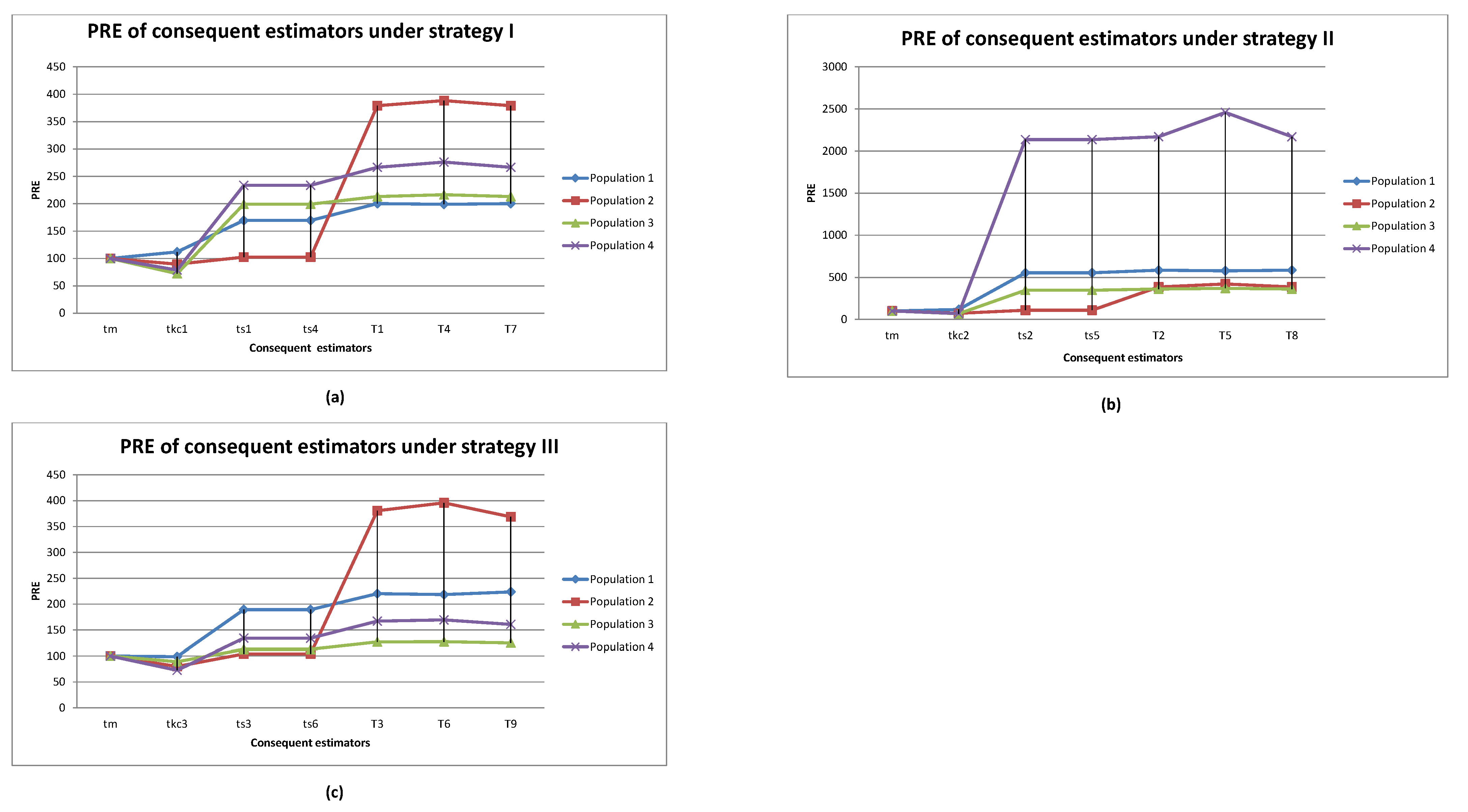
where , and . The results of the numerical analysis are summarized in Table 2 and depicted in Figure 1 under strategies I, II, III and III for each population.
6.2. Simulation Analysis
To assess the performance of the suggested imputation methods, following [27], simulation experiments were conducted over three parent populations, namely, Normal, Gamma, and Weibull, of size units with variables X and Y, expressed by
where and are independent variables of the corresponding parent population. The sampling methodology of Section 2 was used to draw an RSS of size 12 units with set size 3 from each parent population. Using 20,000 iterations, the PRE of the consequent estimators compared to the conventional mean estimator were computed as
6.3. Discussion of Computational Findings
After carefully observing the findings reported in Table 2, Table 3, Table 4, Table 5, Table 6, Table 7, Table 8 and Table 9, we discuss the following points:
- (i).
- From the findings of Table 2, the proposed imputation methods , outperform the mean imputation methods, ref. [21] imputation methods and ref. [22] imputation methods in each real population. Furthermore, the proposed imputation methods , were superior among the proposed imputation methods in population 1, whereas the proposed imputation methods , were superior among the proposed imputation methods in populations 2–4. This is easily observed in Figure 1.
- (ii).
- From the findings of Table 3, Table 4, Table 5, Table 6, Table 7, Table 8 and Table 9, the proposed imputation methods , are also better than the mean imputation, ref. [21] imputation methods and ref. [22] imputation methods under both the symmetric and asymmetric populations for different correlation coefficients , coefficients of skewness and coefficients of kurtosis
- (iii).
- When the parent population was normal (symmetric) and Weibull (asymmetric), the proposed ratio-type imputation methods , always performed better than the competitors as well as within the proposed class of imputation methods under strategies I, II and III.
- (iv).
- When the parent population was Gamma (asymmetric), the proposed difference- and ratio-type imputation methods , were equally efficient and outperformed the conventional methods and performed better in comparison with the proposed imputation methods under strategies I, II and III.
- (v).
- The suggested imputation methods performed better in strategy II compared to strategies I and III in the real and artificially generated populations.
- (vi).
- It can be easily seen that the PRE decreases with the increase in asymmetry and peakedness for asymmetric distributions such as Gamma and Weibull.
- (vii).
- Moreover, the numerical analysis is summarized in Table 2 and Figure 1 under strategies I, II, and III for real populations 1–4. The PRE of the consequent estimators for the remaining simulation results in Table 3, Table 4, Table 5, Table 6 and Table 7 exhibit the same pattern and can be easily presented as line diagrams, if required.
7. Conclusions
In this manuscript, we proposed efficient difference- and ratio-type imputation methods for the estimation of the population mean in the presence of missing data. The efficiency conditions have been derived and sustained with computational analysis on some real and hypothetically generated symmetric and asymmetric populations. The computational and theoretical results show that the proposed imputation methods outperformed the mean imputation method , ref. [21] imputation methods , i = 1, 2, 3, and ref. [22] imputation methods , .
In the simulation analysis, we considered one family of a symmetric population, namely, Normal, and two families of asymmetric populations, namely, Gamma and Weibull, to ascertain the effect of the correlation coefficient for a symmetric population and the effect of skewness and kurtosis for asymmetric populations.
It is worth mentioning that among the asymmetric populations, all imputation methods exhibited a decreasing trend in PRE as the coefficient of skewness and kurtosis increased. Although, in such cases, the proposed estimators fared better than their conventional counterparts. These results are in agreement with the results of [17,28,29], where these authors took skewed distributions and reported that the efficiency of the estimators decreased with an increase in skewness and kurtosis. The same was also true for imputation as well.
Lastly, the proposed imputation methods currently provide the best possible imputation methods for the estimation of a population mean in the presence of the missing data.
Furthermore, the proposed imputation strategies can be defined using multi-auxiliary information, which our future research with investigate.
Author Contributions
Supervision, S.B.; conceptualization, S.B. and A.K.; methodology, S.B. and A.K.; software, A.K.; validation, S.B.; writing—original draft preparation, A.K.; writing—review and editing, A.K., S.B., T.Z. and A.A.M.; Funding, T.Z. and A.A.M. All authors have read and agreed to the published version of the manuscript.
Funding
This research is supported by researchers supporting project number (PNURSP2023R368), Princess Nourah bint Abdulrahman University, Riyadh, Saudi Arabia.
Data Availability Statement
The article includes all data utilized for this investigation.
Acknowledgments
Princess Nourah bint Abdulrahman University Researchers Supporting Project number (PNURSP2023R368), Princess Nourah bint Abdulrahman University, Riyadh, Saudi Arabia.
Conflicts of Interest
The authors declare no conflict of interest.
Appendix A
The expressions of , minimum , and the optimum scalar values of the existing resultant estimators is reported below.
To obtain the minimum , the optimum scalar values associated with the estimators discussed in Section 3 are given below.
, , ,
Appendix B
In this section, we outline the proof of Theorem 1 and Corollary 1.
Under strategy I, consider the estimator
Using the notations discussed in the earlier section, we obtain
Squaring both sides of (A11) and taking the expectation, we obtain the of the estimator as
The optimum values of and can be obtained by minimizing (A12) with respect to and as
Introducing and into (A12), we obtain the minimum as
Similarly, we can obtain the optimum values of constants and minimum of other proposed estimators, which are
where
References
- Rubin, R.B. Inference and missing data. Biometrika 1976, 63, 581–592. [Google Scholar] [CrossRef]
- Lee, H.; Rancourt, E.; Sarndal, C.E. Experiments with variance estimation from survey data with imputed values. J. Off. Stat. 1994, 10, 231–243. [Google Scholar]
- Singh, S.; Horn, S. Compromised imputation in survey sampling. Metrika 2000, 51, 267–276. [Google Scholar] [CrossRef]
- Singh, S.; Deo, B. Imputation by power transformation. Stat. Pap. 2003, 44, 555–579. [Google Scholar] [CrossRef]
- Singh, S. A new method of imputation in survey sampling. Stat. A J. Theor. Appl. Stat. 2009, 43, 499–511. [Google Scholar] [CrossRef]
- Singh, S.; Valdes, S.R. Optimal method of imputation in survey sampling. Appl. Math. Sci. 2009, 3, 1727–1737. [Google Scholar]
- Heitjan, D.F.; Basu, S. Distinguishing ‘Missing at Random’ and ‘Missing Completely at Random’. Am. Stat. 1996, 50, 207–213. [Google Scholar]
- Ahmed, M.S.; Al-Titi, O.; Al-Rawi, Z.; Abu-Dayyeh, W. Estimation of a population mean using different imputation methods. Stat. Transit. 2006, 7, 1247–1264. [Google Scholar]
- Kadilar, C.; Cingi, H. Estimators for the population mean in the case of missing data. Commun. Stat. Theory Methods 2008, 37, 2226–2236. [Google Scholar] [CrossRef]
- Diana, G.; Perri, P.F. Improved estimators of the population mean for missing data. Commun. Stat. Theory Methods 2010, 39, 3245–3251. [Google Scholar] [CrossRef]
- Bhushan, S.; Pandey, A.P. Optimal imputation of missing data for estimation of population mean. J. Stat. Manag. Syst. 2016, 19, 755–769. [Google Scholar] [CrossRef]
- Bhushan, S.; Pandey, A.P. Optimality of ratio type estimation methods for population mean in presence of missing data. Commun. Stat. Theory Methods 2018, 47, 2576–2589. [Google Scholar] [CrossRef]
- Bhushan, S.; Pandey, A.P.; Pandey, A. On optimality of imputation methods for estimation of population mean using higher order moments of an auxiliary variable. Commun. Stat. Simul. Comput. 2018, 49, 1–15. [Google Scholar] [CrossRef]
- Mohamed, C.; Sedory, S.A.; Singh, S. Imputation using higher order moments of an auxiliary variable. Commun. Stat. Simul. Comput. 2016, 46, 6588–6617. [Google Scholar] [CrossRef]
- Bhushan, S.; Kumar, A.; Pandey, A.P.; Singh, S. Estimation of population mean in presence of missing data under simple random sampling. Commun. Stat. Simul. Comput. 2022, 1–22. [Google Scholar] [CrossRef]
- Anas, M.M.; Huang, Z.; Shahzad, U.; Zaman, T.; Shahzadi, S. Compromised imputation based mean estimators using robust quantile regression. Commun. Stat. Theory Methods 2022, 1–16. [Google Scholar] [CrossRef]
- McIntyre, G.A. A method of unbiased selective sampling using ranked set. Aust. J. Agric. Res. 1952, 3, 385–390. [Google Scholar] [CrossRef]
- Takahasi, K.; Wakimoto, K. On unbiased estimates of the population mean based on the sample stratified by means of ordering. Ann. Inst. Stat. Math. 1968, 20, 1–31. [Google Scholar] [CrossRef]
- Bouza Herrera, C.N.; Al-Omari, A.I. Ranked set estimation with imputation of the missing observations: The median estimator. Rev. Investig. Oper. 2011, 32, 30–37. [Google Scholar]
- Bouza, C.N. Handling Missing Data in Ranked Set Sampling; Springer: Berlin/Heidelberg, Germany, 2013. [Google Scholar]
- Al-Omari, A.; Bouza, C. Ratio estimators of the population mean with missing values using ranked set sampling. Environmetrics 2014, 26, 67–76. [Google Scholar] [CrossRef]
- Sohail, M.U.; Shabbir, J.; Ahmed, S. A class of ratio type estimators for imputing the missing values under rank set sampling. J. Stat. Theory Pract. 2018, 12, 704–717. [Google Scholar] [CrossRef]
- Arnold, B.C.; Balakrishnan, N.; Nagaraja, H.N. A First Course in Order Statistics; Wiley: New York, NY, USA, 1993. [Google Scholar]
- Kadilar, C.; Cingi, H. Ratio estimators in stratified random sampling. Biom. J. 2003, 45, 218–225. [Google Scholar] [CrossRef]
- Sarndal, C.E.; Swensson, B.; Wretman, J. Model Assisted Survey Sampling; Springer: New York, NY, USA, 2003. [Google Scholar]
- Singh, S. Advanced Sampling Theory with Applications: How Michael Selected Amy; Kluwer: Amsterdam, The Netherlands, 2003; Volumes 1 and 2. [Google Scholar]
- Singh, S.; Horn, S. An alternative survey in multi-character survey. Metrika 1998, 48, 99–107. [Google Scholar] [CrossRef]
- Dell, T.R.; Clutter, J.L. Ranked set sampling theory with order statistics background. Biometrics 1972, 28, 545–555. [Google Scholar] [CrossRef]
- Bhushan, S.; Kumar, A. Novel log type class of estimators under ranked set sampling. Sankhya B 2022, 84, 421–447. [Google Scholar] [CrossRef]
Figure 1.
PRE results of the consequent estimators under (a) strategy I, (b) strategy II, and (c) strategy III for the real populations reported in Table 2.
Figure 1.
PRE results of the consequent estimators under (a) strategy I, (b) strategy II, and (c) strategy III for the real populations reported in Table 2.


Table 1.
Description of the population parameters.
| Parameters | Population 1 | Population 2 | Population 3 | Population 4 |
|---|---|---|---|---|
| N | 69 | 124 | 50 | 284 |
| n | 12 | 12 | 12 | 12 |
| m | 3 | 3 | 3 | 3 |
| r | 4 | 4 | 4 | 4 |
| P | 0.5 | 0.3 | 0.7 | 0.6 |
| 71.34 | 36.65 | 555.43 | 47.50 | |
| 3165.02 | 14276.03 | 878.16 | 9.05 | |
| 110.85 | 116.80 | 584.82 | 11.06 | |
| 3965.24 | 31431.81 | 1084677 | 4.95 | |
| 0.91 | 0.23 | 0.80 | 0.66 |
Table 2.
PRE of the proposed estimators for real populations.
| Estimators | Population 1 | Population 2 | Population 3 | Population 4 |
|---|---|---|---|---|
| 100.00 | 100.00 | 100.00 | 100.00 | |
| Strategy I | ||||
| 200.23 | 379.07 | 213.14 | 266.61 | |
| 198.93 | 388.40 | 216.47 | 276.07 | |
| 200.23 | 379.07 | 213.14 | 266.61 | |
| , i = 1, 4 | 169.41 | 102.59 | 199.16 | 233.60 |
| 111.93 | 89.60 | 72.25 | 78.77 | |
| Strategy II | ||||
| 584.83 | 385.66 | 360.33 | 2169.67 | |
| 576.85 | 421.37 | 369.29 | 2459.06 | |
| 584.83 | 385.66 | 360.33 | 2169.67 | |
| , i = 2, 5 | 554.02 | 109.18 | 346.35 | 2136.65 |
| 118.15 | 72.99 | 68.44 | 69.78 | |
| Strategy III | ||||
| 220.06 | 380.63 | 126.93 | 167.17 | |
| 218.39 | 395.85 | 127.34 | 169.46 | |
| 223.56 | 368.69 | 125.09 | 160.86 | |
| , i = 3, 6 | 189.24 | 104.14 | 112.94 | 134.15 |
| 98.91 | 79.99 | 89.12 | 72.58 |
Table 3.
PRE of the proposed estimators at P = 0.20.
| 0.6 | 0.7 | 0.8 | 0.9 | |
|---|---|---|---|---|
| 100 | 100 | 100 | 100 | |
| Strategy I | ||||
| 108.2314 | 110.1882 | 113.1969 | 118.9193 | |
| 108.9253 | 110.9860 | 114.1003 | 119.9397 | |
| , i = 1, 4 | 102.4440 | 102.7442 | 102.8370 | 102.7567 |
| 56.3365 | 62.5280 | 70.0558 | 78.6946 | |
| Strategy II | ||||
| , i = 2, 8 | 119.3313 | 122.8567 | 126.3605 | 131.6545 |
| 123.7161 | 127.9222 | 132.0179 | 137.8729 | |
| , i = 2, 5 | 113.5438 | 115.4126 | 116.0005 | 115.492 |
| 20.5860 | 25.1720 | 32.1576 | 43.0168 | |
| Strategy III | ||||
| 116.3368 | 119.4054 | 122.7634 | 128.1837 | |
| 119.6366 | 123.2108 | 127.0276 | 132.9048 | |
| , i = 3, 6 | 110.5493 | 111.9614 | 112.4035 | 112.0212 |
| 21.7699 | 27.3798 | 35.9864 | 49.5031 | |
| Skewness of Y | 0.6046 | 0.6134 | 0.6571 | 0.7487 |
| Kurtosis of Y | 3.4184 | 3.4308 | 3.5393 | 3.7750 |
| Strategy I | ||||
| , | 104.1361 | 104.0201 | 103.8752 | 103.7148 |
| 103.9699 | 103.8591 | 103.7210 | 103.5712 | |
| , i = 1, 4 | 102.2484 | 102.1062 | 101.8782 | 101.5178 |
| 84.4838 | 84.5867 | 85.0399 | 86.0938 | |
| Strategy II | ||||
| , i = 2, 8 | 114.2407 | 113.4139 | 112.1508 | 110.2765 |
| 113.4229 | 112.6215 | 111.3919 | 109.5685 | |
| , i = 2, 5 | 112.3531 | 111.5000 | 110.1539 | 108.0795 |
| 52.5444 | 52.7365 | 53.6026 | 55.6966 | |
| Strategy III | ||||
| 111.5319 | 110.9071 | 109.9584 | 108.5579 | |
| 110.8735 | 110.2693 | 109.3479 | 107.9888 | |
| , i = 3, 6 | 109.6442 | 108.9931 | 107.9614 | 106.3608 |
| 50.0729 | 50.1878 | 50.9778 | 52.9983 | |
| Skewness of Y | 1.3561 | 1.3526 | 1.4714 | 1.7607 |
| Kurtosis of Y | 5.2276 | 5.2844 | 6.0535 | 7.8079 |
| Strategy I | ||||
| , i = 1, 7 | 107.3833 | 107.2255 | 107.1537 | 107.1449 |
| 107.5074 | 107.3496 | 107.2772 | 107.2674 | |
| , i = 1, 4 | 105.6587 | 105.0803 | 104.5253 | 103.9469 |
| 80.5933 | 83.9483 | 86.6202 | 88.7951 | |
| Strategy II | ||||
| , i = 2, 8 | 138.2957 | 134.0250 | 130.2555 | 126.6323 |
| 139.1752 | 134.8628 | 131.0549 | 127.3948 | |
| , i = b2, 5 | 136.5711 | 131.8799 | 127.6271 | 123.4344 |
| 46.4315 | 52.3644 | 57.8042 | 62.7748 | |
| Strategy III | ||||
| 128.9875 | 126.1204 | 123.5728 | 121.1061 | |
| 129.6256 | 126.7374 | 124.1689 | 121.6812 | |
| , i = 3, 6 | 127.2628 | 123.9752 | 120.9444 | 117.9082 |
| 55.5027 | 62.5806 | 68.7953 | 74.1058 |
Bold values indicate maximum PRE.
Table 4.
PRE of the proposed estimators at P = 0.30.
| 0.6 | 0.7 | 0.8 | 0.9 | |
|---|---|---|---|---|
| 100 | 100 | 100 | 100 | |
| Strategy I | ||||
| , i = 1, 7 | 107.5696 | 109.1362 | 111.2233 | 114.9679 |
| 108.2824 | 109.9559 | 112.1497 | 116.0109 | |
| , i = 1, 4 | 103.7113 | 104.1735 | 104.3167 | 104.1929 |
| 46.2412 | 52.6613 | 60.9329 | 71.1186 | |
| Strategy II | ||||
| , i = 2, 8 | 117.4021 | 120.3753 | 122.9071 | 126.2670 |
| 120.3133 | 123.7369 | 126.6603 | 130.3914 | |
| , i = 2, 5 | 113.5438 | 115.4126 | 116.0005 | 115.4920 |
| 20.5860 | 25.1720 | 32.1576 | 43.0168 | |
| Strategy III | ||||
| 112.9688 | 115.2747 | 117.5940 | 121.1378 | |
| 114.8323 | 117.4214 | 120.0030 | 123.8138 | |
| , i = 3, 6 | 109.1105 | 110.3120 | 110.6873 | 110.3628 |
| 21.7699 | 27.3798 | 35.9864 | 49.5031 | |
| Skewness of Y | 0.6046 | 0.6134 | 0.6571 | 0.7487 |
| Kurtosis of Y | 3.4184 | 3.4308 | 3.5393 | 3.7750 |
| Strategy I | ||||
| , i = 1, 7 | 104.6694 | 104.4689 | 104.1753 | 103.7588 |
| 104.5033 | 104.3080 | 104.0213 | 103.6153 | |
| , i = 1, 4 | 103.4110 | 103.1930 | 102.8440 | 102.2941 |
| 78.4014 | 78.5344 | 79.1216 | 80.4968 | |
| Strategy II | ||||
| , i = 2, 8 | 113.6115 | 112.7759 | 111.4852 | 109.5442 |
| 113.0660 | 112.2474 | 110.9790 | 109.0720 | |
| , i = 2, 5 | 112.3531 | 111.5000 | 110.1539 | 108.0795 |
| 52.5444 | 52.7365 | 53.6026 | 55.6966 | |
| Strategy III | ||||
| 109.5966 | 109.0575 | 108.2289 | 106.9865 | |
| 109.2114 | 108.6844 | 107.8719 | 106.6538 | |
| , i = 3, 6 | 108.3381 | 107.7815 | 106.8976 | 105.5218 |
| 50.0729 | 50.1878 | 50.9778 | 52.9983 | |
| Skewness of Y | 1.3561 | 1.3526 | 1.4714 | 1.7607 |
| Kurtosis of Y | 5.2276 | 5.2844 | 6.0535 | 7.8079 |
| Strategy I | ||||
| , i = 1, 7 | 109.8849 | 109.2492 | 108.6973 | 108.1715 |
| 110.0138 | 109.3775 | 108.8245 | 108.2972 | |
| , i = 1, 4 | 108.7352 | 107.8191 | 106.9450 | 106.0396 |
| 73.4648 | 77.7113 | 81.1888 | 84.0843 | |
| Strategy II | ||||
| , i = 2, 8 | 137.7209 | 133.3100 | 129.3794 | 125.5664 |
| 138.3068 | 133.8682 | 129.9120 | 126.0744 | |
| , i = 2, 5 | 136.5711 | 131.8799 | 127.6271 | 123.4344 |
| 46.4315 | 52.3644 | 57.8042 | 62.7748 | |
| Strategy III | ||||
| 124.2186 | 121.7980 | 119.6111 | 117.4585 | |
| 124.574 | 122.1439 | 119.9472 | 117.7845 | |
| , i = 3, 6 | 123.0688 | 120.3679 | 117.8588 | 115.3266 |
| 55.5027 | 62.5806 | 68.7953 | 74.1058 |
Bold values indicate maximum PRE.
Table 5.
PRE of the proposed estimators at P = 0.40.
| 0.6 | 0.7 | 0.8 | 0.9 | |
|---|---|---|---|---|
| 100 | 100 | 100 | 100 | |
| Strategy I | ||||
| , | 107.9041 | 109.3652 | 111.0196 | 113.7510 |
| 108.6366 | 110.2077 | 111.9699 | 114.8175 | |
| , | 105.0104 | 105.6432 | 105.8396 | 105.6698 |
| 39.2142 | 45.4841 | 53.9122 | 64.8732 | |
| Strategy II | ||||
| , | 116.4375 | 119.1347 | 121.1805 | 123.5733 |
| 118.6164 | 121.6501 | 123.9885 | 126.6586 | |
| , | 113.5438 | 115.4126 | 116.0005 | 115.4920 |
| 20.5860 | 25.1720 | 32.1576 | 43.0168 | |
| Strategy III | ||||
| 110.6024 | 112.4326 | 114.2028 | 116.8341 | |
| 111.7649 | 113.7708 | 115.7070 | 118.5106 | |
| , | 107.7087 | 108.7106 | 109.0228 | 108.7528 |
| 21.7699 | 27.3798 | 35.9864 | 49.5031 | |
| Skewness of Y | 0.6046 | 0.6134 | 0.6571 | 0.7487 |
| Kurtosis of Y | 3.4184 | 3.4308 | 3.5393 | 3.7750 |
| Strategy I | ||||
| , | 105.5441 | 105.2600 | 104.8268 | 104.1809 |
| 105.3782 | 105.0993 | 104.6730 | 104.0376 | |
| , | 104.6003 | 104.3031 | 103.8283 | 103.0824 |
| 73.1359 | 73.2903 | 73.9734 | 75.5831 | |
| Strategy II | ||||
| , | 113.2969 | 112.4569 | 111.1524 | 109.1780 |
| 112.8877 | 112.0605 | 110.7727 | 108.8238 | |
| , | 112.3531 | 111.5000 | 110.1539 | 108.0795 |
| 52.5444 | 52.7365 | 53.6026 | 55.6966 | |
| Strategy III | ||||
| 108.0067 | 107.5535 | 106.8530 | 105.7945 | |
| 107.7585 | 107.3131 | 106.6230 | 105.5802 | |
| , | 107.0628 | 106.5965 | 105.8546 | 104.6959 |
| 50.0729 | 50.1878 | 50.9778 | 52.9983 | |
| Skewness of Y | 1.3561 | 1.3526 | 1.4714 | 1.7607 |
| Kurtosis of Y | 5.2276 | 5.2844 | 6.0535 | 7.8079 |
| Strategy I | ||||
| , | 112.8585 | 111.7770 | 110.7937 | 109.8172 |
| 112.9926 | 111.9098 | 110.9247 | 109.9461 | |
| , | 111.9962 | 110.7044 | 109.4795 | 108.2182 |
| 67.4948 | 72.3369 | 76.3983 | 79.8482 | |
| Strategy II | ||||
| , | 137.4334 | 132.9525 | 128.9413 | 125.0334 |
| 137.8727 | 133.3710 | 129.3406 | 125.4143 | |
| , | 136.5711 | 131.8799 | 127.6271 | 123.4344 |
| 46.4315 | 52.3644 | 57.8042 | 62.7748 | |
| Strategy III | ||||
| 120.0047 | 118.0372 | 116.2409 | 114.4546 | |
| 120.2233 | 118.2512 | 116.4501 | 114.6584 | |
| , | 119.1424 | 116.9646 | 114.9267 | 112.8556 |
| 55.5027 | 62.5806 | 68.7953 | 74.1058 |
Bold values indicate maximum PRE.
Table 6.
PRE of the proposed estimators at P = 0.50.
| 0.6 | 0.7 | 0.8 | 0.9 | |
|---|---|---|---|---|
| 100 | 100 | 100 | 100 | |
| Strategy I | ||||
| , | 108.6574 | 110.1325 | 111.5516 | 113.6541 |
| 109.4103 | 110.9988 | 112.5270 | 114.7449 | |
| , | 106.3424 | 107.1549 | 107.4076 | 107.1891 |
| 34.0412 | 40.0286 | 48.3422 | 59.6361 | |
| Strategy II | ||||
| , | 115.8588 | 118.3903 | 120.1445 | 121.9570 |
| 117.5997 | 120.3998 | 122.3876 | 124.4215 | |
| , | 113.5438 | 115.4126 | 116.0005 | 115.4920 |
| 20.5860 | 25.1720 | 32.1576 | 43.0168 | |
| Strategy III | ||||
| 108.6574 | 110.1325 | 111.5516 | 113.6541 | |
| 109.4103 | 110.9988 | 112.5270 | 114.7449 | |
| , | 106.3424 | 107.1549 | 107.4076 | 107.1891 |
| 21.7699 | 27.3798 | 35.9864 | 49.5031 | |
| Skewness of Y | 0.6046 | 0.6134 | 0.6571 | 0.7487 |
| Kurtosis of Y | 3.4184 | 3.4308 | 3.5393 | 3.7750 |
| Strategy I | ||||
| , | 106.5723 | 106.2029 | 105.6304 | 104.7617 |
| 106.4066 | 106.0424 | 105.4768 | 104.6186 | |
| , | 105.8172 | 105.4373 | 104.8316 | 103.8829 |
| 68.5332 | 68.7027 | 69.4543 | 71.2347 | |
| Strategy II | ||||
| , | 113.1081 | 112.2655 | 110.9527 | 108.9583 |
| 112.7807 | 111.9483 | 110.6489 | 108.6749 | |
| , | 112.3531 | 111.5000 | 110.1539 | 108.0795 |
| 52.5444 | 52.7365 | 53.6026 | 55.6966 | |
| Strategy III | ||||
| 106.5723 | 106.2029 | 105.6304 | 104.7617 | |
| 106.4066 | 106.0424 | 105.4768 | 104.6186 | |
| , | 105.8172 | 105.4373 | 104.8316 | 103.8829 |
| 50.0729 | 50.1878 | 50.9778 | 52.9983 | |
| Skewness of Y | 1.3561 | 1.3526 | 1.4714 | 1.7607 |
| Kurtosis of Y | 5.2276 | 5.2844 | 6.0535 | 7.8079 |
| Strategy I | ||||
| , | 116.1487 | 114.6065 | 113.1884 | 113.1884 |
| 116.2883 | 114.7441 | 113.3234 | 113.3234 | |
| , | 115.4588 | 113.7484 | 112.1370 | 112.1370 |
| 62.4222 | 67.6579 | 72.1416 | 72.1416 | |
| Strategy II | ||||
| , | 137.2610 | 132.7379 | 128.6785 | 128.6785 |
| 137.6123 | 133.0727 | 128.9979 | 128.9979 | |
| , | 136.5711 | 131.8799 | 127.6271 | 127.6271 |
| 46.4315 | 52.3644 | 57.8042 | 57.8042 | |
| Strategy III | ||||
| 116.1487 | 114.6065 | 113.1884 | 111.7674 | |
| 116.2883 | 114.7441 | 113.3234 | 111.8997 | |
| , | 115.4588 | 113.7484 | 112.137 | 110.4883 |
| 55.5027 | 62.5806 | 68.7953 | 68.7953 |
Bold values indicate maximum PRE.
Table 7.
PRE of the proposed estimators at P = 0.60.
| 0.6 | 0.7 | 0.8 | 0.9 | |
|---|---|---|---|---|
| 100 | 100 | 100 | 100 | |
| Strategy I | ||||
| , | 109.6378 | 111.1919 | 112.4761 | 114.1403 |
| 110.4120 | 112.0830 | 113.4776 | 115.2564 | |
| , | 107.7087 | 108.7106 | 109.0228 | 108.7528 |
| 30.0739 | 35.7417 | 43.8154 | 55.1814 | |
| Strategy II | ||||
| , | 115.4729 | 117.8940 | 119.4538 | 120.8795 |
| 116.9226 | 119.5671 | 121.3212 | 122.9311 | |
| , | 113.5438 | 115.4126 | 116.0005 | 115.4920 |
| 20.5860 | 25.1720 | 32.1576 | 43.0168 | |
| Strategy III | ||||
| 106.9395 | 108.1245 | 109.2929 | 111.0573 | |
| 107.4275 | 108.6858 | 109.926 | 111.7676 | |
| , | 105.0104 | 105.6432 | 105.8396 | 105.6698 |
| 21.7699 | 27.3798 | 35.9864 | 49.5031 | |
| Skewness of Y | 0.6046 | 0.6134 | 0.6571 | 0.7487 |
| Kurtosis of Y | 3.4184 | 3.4308 | 3.5393 | 3.7750 |
| Strategy I | ||||
| , | 107.6921 | 107.2345 | 106.5202 | 105.4283 |
| 107.5266 | 107.0743 | 106.3668 | 105.2854 | |
| , | 107.0628 | 106.5965 | 105.8546 | 104.6959 |
| 64.4756 | 64.6556 | 65.4555 | 67.3595 | |
| Strategy II | ||||
| , | 112.9823 | 112.1380 | 110.8195 | 108.8119 |
| 112.7094 | 111.8736 | 110.5664 | 108.5756 | |
| , | 112.3531 | 111.5000 | 110.1539 | 108.0795 |
| 52.5444 | 52.7365 | 53.6026 | 55.6966 | |
| Strategy III | ||||
| 105.2295 | 104.9411 | 104.4940 | 103.8147 | |
| 105.1188 | 104.8339 | 104.3914 | 103.7192 | |
| , | 104.6003 | 104.3031 | 103.8283 | 103.0824 |
| 50.0729 | 50.1878 | 50.9778 | 52.9983 | |
| Skewness of Y | 1.3561 | 1.3526 | 1.4714 | 1.7607 |
| Kurtosis of Y | 5.2276 | 5.2844 | 6.0535 | 7.8079 |
| Strategy I | ||||
| , | 119.7173 | 117.6797 | 115.8029 | 113.9216 |
| 119.8630 | 117.8223 | 115.9423 | 114.0574 | |
| , | 119.1424 | 116.9646 | 114.9267 | 112.8556 |
| 58.0588 | 63.5474 | 68.3343 | 72.5392 | |
| Strategy II | ||||
| , | 137.1460 | 132.5949 | 128.5032 | 124.5004 |
| 137.4387 | 132.8739 | 128.7694 | 124.7542 | |
| , | 136.5711 | 131.8799 | 127.6271 | 123.4344 |
| 46.4315 | 52.3644 | 57.8042 | 62.7748 | |
| Strategy III | ||||
| 112.571 | 111.4195 | 110.3556 | 109.2842 | |
| 112.6604 | 111.5080 | 110.4430 | 109.3701 | |
| , | 111.9962 | 110.7044 | 109.4795 | 108.2182 |
| 55.5027 | 62.5806 | 68.7953 | 74.1058 |
Bold values indicate maximum PRE.
Table 8.
PRE of the proposed estimators at P = 0.70.
| 0.6 | 0.7 | 0.8 | 0.9 | |
|---|---|---|---|---|
| 100 | 100 | 100 | 100 | |
| Strategy I | ||||
| , | 110.7640 | 112.4389 | 113.6473 | 114.9807 |
| 111.5604 | 113.3559 | 114.6761 | 116.1231 | |
| , | 109.1105 | 110.3120 | 110.6873 | 110.3628 |
| 26.9348 | 32.2841 | 40.0638 | 51.3460 | |
| Strategy II | ||||
| , | 115.1973 | 117.5395 | 118.9605 | 120.1099 |
| 116.4391 | 118.9727 | 120.5600 | 121.8671 | |
| , | 113.5438 | 115.4126 | 116.0005 | 115.4929 |
| 20.5860 | 25.1720 | 32.1576 | 43.0168 | |
| Strategy III | ||||
| 105.3648 | 106.3004 | 107.2767 | 108.8108 | |
| 105.6700 | 106.6513 | 107.6731 | 109.2571 | |
| , | 103.7113 | 104.1735 | 104.3167 | 104.1929 |
| 21.7699 | 27.3798 | 35.9864 | 49.5031 | |
| Skewness of Y | 0.6046 | 0.6134 | 0.6571 | 0.7487 |
| Kurtosis of Y | 3.4184 | 3.4308 | 3.5393 | 3.7750 |
| Strategy I | ||||
| , | 108.8775 | 108.3284 | 107.4682 | 106.1495 |
| 108.7123 | 108.1684 | 107.3151 | 106.0069 | |
| , | 108.3381 | 107.7815 | 106.8976 | 105.5218 |
| 60.8715 | 61.0588 | 61.8921 | 63.8842 | |
| Strategy II | ||||
| , | 112.8924 | 112.0468 | 110.7245 | 108.7072 |
| 112.6585 | 111.8202 | 110.5074 | 108.5048 | |
| , | 112.3531 | 111.5000 | 110.1539 | 108.0795 |
| 52.5444 | 52.7365 | 53.6026 | 55.6966 | |
| Strategy III | ||||
| 103.9503 | 103.7398 | 103.4146 | 102.9218 | |
| 103.8791 | 103.6708 | 103.3486 | 102.8603 | |
| , | 103.4110 | 103.1930 | 102.844 | 102.2941 |
| 50.0729 | 50.1878 | 50.9778 | 52.9983 | |
| Skewness of Y | 1.3561 | 1.3526 | 1.4714 | 1.7607 |
| Kurtosis of Y | 5.2276 | 5.2844 | 6.0535 | 7.8079 |
| Strategy I | ||||
| , | 123.5616 | 120.9808 | 118.6098 | 116.2403 |
| 123.7138 | 121.1290 | 118.7538 | 116.3799 | |
| 123.0688 | 120.3679 | 117.8588 | 115.3266 | |
| 54.2655 | 59.9077 | 64.9087 | 69.3645 | |
| Strategy II | ||||
| , | 137.0639 | 132.4928 | 128.3781 | 124.3481 |
| 137.3148 | 132.7318 | 128.6062 | 124.5657 | |
| , | 136.5711 | 131.8799 | 127.6271 | 123.4344 |
| 46.4315 | 52.3644 | 57.8042 | 62.7748 | |
| Strategy III | ||||
| 109.2279 | 108.432 | 107.696 | 106.9533 | |
| 109.2831 | 108.4869 | 107.7505 | 107.0071 | |
| , | 108.7352 | 107.8191 | 106.945 | 106.0396 |
| 55.5027 | 62.5806 | 68.7953 | 74.1058 |
Bold values indicate maximum PRE.
Table 9.
PRE of the proposed estimators at P = 0.80.
| 0.6 | 0.7 | 0.8 | 0.9 | |
|---|---|---|---|---|
| 100 | 100 | 100 | 100 | |
| Strategy I | ||||
| , | 111.9961 | 113.8224 | 114.9935 | 116.0618 |
| 112.8155 | 114.7665 | 116.0507 | 117.2317 | |
| 110.5493 | 111.9614 | 112.4035 | 112.0212 | |
| 24.3891 | 29.4365 | 36.9040 | 48.0091 | |
| Strategy II | ||||
| , | 114.9907 | 117.2736 | 118.5905 | 119.5327 |
| 116.0767 | 118.5271 | 119.9893 | 121.0694 | |
| 113.5438 | 115.4126 | 116.0005 | 115.4920 | |
| 20.5860 | 25.1720 | 32.1576 | 43.0168 | |
| Strategy III | ||||
| 103.8908 | 104.6052 | 105.427 | 106.7974 | |
| 104.0641 | 104.8043 | 105.6524 | 107.052 | |
| , | 102.444 | 102.7442 | 102.8370 | 102.7567 |
| 21.7699 | 27.3798 | 35.9864 | 49.5031 | |
| Skewness of Y | 0.6046 | 0.6134 | 0.6571 | 0.7487 |
| Kurtosis of Y | 3.4184 | 3.4308 | 3.5393 | 3.7750 |
| Strategy I | ||||
| , | 110.1161 | 109.4716 | 108.4607 | 106.9101 |
| 109.9513 | 109.3120 | 108.3079 | 106.7677 | |
| , | 109.6442 | 108.9931 | 107.9614 | 106.3608 |
| 57.6491 | 57.8411 | 58.6967 | 60.7498 | |
| Strategy II | ||||
| , | 112.8250 | 111.9785 | 110.6531 | 108.6288 |
| 112.6203 | 111.7802 | 110.4632 | 108.4516 | |
| , | 112.3531 | 111.5000 | 110.1539 | 108.0795 |
| 52.5444 | 52.7365 | 53.6026 | 55.6966 | |
| Strategy III | ||||
| 102.7203 | 102.5847 | 102.3774 | 102.0671 | |
| 102.6788 | 102.5444 | 102.3389 | 102.0311 | |
| , | 102.2484 | 102.1062 | 101.8782 | 101.5178 |
| 50.0729 | 50.1878 | 50.9778 | 52.9983 | |
| Skewness of Y | 1.3561 | 1.3526 | 1.4714 | 1.7607 |
| Kurtosis of Y | 5.2276 | 5.2844 | 6.0535 | 7.8079 |
| Strategy I | ||||
| , | 127.6940 | 124.5115 | 121.6015 | 118.7077 |
| 127.8533 | 124.6656 | 121.7504 | 118.8513 | |
| , | 127.2628 | 123.9752 | 120.9444 | 117.9082 |
| 50.9375 | 56.6624 | 61.8101 | 66.4561 | |
| Strategy II | ||||
| , | 137.0023 | 132.4162 | 128.2842 | 124.2339 |
| 137.2218 | 132.6253 | 128.4838 | 124.4243 | |
| , | 136.5711 | 131.8799 | 127.6271 | 123.4344 |
| 46.4315 | 52.3644 | 57.8042 | 62.7748 | |
| Strategy III | ||||
| 106.0898 | 105.6166 | 105.1824 | 104.7464 | |
| 106.1208 | 105.6476 | 105.2132 | 104.777 | |
| , | 105.6587 | 105.0803 | 104.5253 | 103.9469 |
| 55.5027 | 62.5806 | 68.7953 | 74.1058 |
Bold values indicate maximum PRE.
Disclaimer/Publisher’s Note: The statements, opinions and data contained in all publications are solely those of the individual author(s) and contributor(s) and not of MDPI and/or the editor(s). MDPI and/or the editor(s) disclaim responsibility for any injury to people or property resulting from any ideas, methods, instructions or products referred to in the content. |
© 2023 by the authors. Licensee MDPI, Basel, Switzerland. This article is an open access article distributed under the terms and conditions of the Creative Commons Attribution (CC BY) license (https://creativecommons.org/licenses/by/4.0/).
Share and Cite
MDPI and ACS Style
Bhushan, S.; Kumar, A.; Zaman, T.; Al Mutairi, A. Efficient Difference and Ratio-Type Imputation Methods under Ranked Set Sampling. Axioms 2023, 12, 558. https://0-doi-org.brum.beds.ac.uk/10.3390/axioms12060558
AMA Style
Bhushan S, Kumar A, Zaman T, Al Mutairi A. Efficient Difference and Ratio-Type Imputation Methods under Ranked Set Sampling. Axioms. 2023; 12(6):558. https://0-doi-org.brum.beds.ac.uk/10.3390/axioms12060558
Chicago/Turabian StyleBhushan, Shashi, Anoop Kumar, Tolga Zaman, and Aned Al Mutairi. 2023. "Efficient Difference and Ratio-Type Imputation Methods under Ranked Set Sampling" Axioms 12, no. 6: 558. https://0-doi-org.brum.beds.ac.uk/10.3390/axioms12060558
Note that from the first issue of 2016, this journal uses article numbers instead of page numbers. See further details here.