Article

Fluid Dynamics Calculation in SF6 Circuit Breaker during Breaking as a Prerequisite for the Digital Twin Creation

by
Vladislav V. Popovtsev
,
Alexandra I. Khalyasmaa
* and
Yurii V. Patrakov
Ural Power Engineering Institute, Ural Federal University Named after the First President of Russia B.N. Yeltsin, 620002 Ekaterinburg, Russia
*
Author to whom correspondence should be addressed.
Submission received: 2 May 2023 / Revised: 12 June 2023 / Accepted: 19 June 2023 / Published: 22 June 2023
(This article belongs to the Special Issue Applied Mathematics in Energy and Mechanical Engineering)

Abstract

:
The requirements to switching the capacities of SF6 circuit breakers submitted by Russian Grid companies are difficult to satisfy. The first limitation is related to material and financial costs in order to create a new requirement-satisfying switching device. The second limitation is dictated by the necessity of calculating complex physical processes in a circuit braker interrupter during fault–current making or breaking before creating a prototype. The latter task is reduced to the problem of simulating the processes of interaction between the switching arc and the SF6 gas flow. This paper deals with the solution of the problem both analytically by a special method and numerically by a numerical software package through the creation of a mathematical model of the interaction process. The switching arc is taken into account as a form of a temperature source, based on experimental data on measuring the temperature of the arc column. The key feature of the research is to use the finite element method based on a moving mesh—the Arbitrary Lagrangian Eulerian (ALE) method. Such a problem statement allows us to take the contact separation curve of the circuit breaker into account as the input data of the model. The calculations were carried out during fault-current breaking by a 110 kV SF6 dead-tank circuit breaker. The calculations of pressure and mass flow in the under-piston volume change, gas flow speed, and temperature depending on the contact separation are given. The proposed model of the switching arc was used to simulate the process of 25 kA symmetrical fault–current breaking and was compared with an experiment.

1. Introduction

The increase in power consumption in the Unified National Power Grid (UNPG) of Russia, along with the expansion of the technical and regulatory framework, quantitatively increases the used equipment or their replacements. One of the most important elements of the Electric Power System (EPS) ensuring its reliability is a such electrical device as a power circuit breaker (CB). Its main tasks are to interrupt short-circuit currents and isolate faulty parts of an EPS. However, conflicting requirements are simultaneously imposed on the CB. On the one hand, during contingencies—fault–current breaking or making—the CB must turn them off and provide an infinitely large resistance between the arcing contacts. On the other hand, under normal conditions, the operating currents through its contact system and its resistance must be infinitely small in order to avoid unnecessary losses of the power to be transmitted [1].
-
Thus, the following requirements are imposed on the CB:
-
Low resistance in normal conditions (in the normally closed contact);
-
High-voltage proof of external and internal insulation, which makes it possible to withstand lightning and switching overvoltage, as well as transient recovering voltage (TRV) after the arc is extinguished;
-
The ability of both making and breaking the short-circuit currents —the CB must reliably extinguish the arc without its re-ignition;
-
Ensuring fast transition from the closed to open position and vice versa, especially in automatic reclosing cycles.
In addition to the short-circuit currents, the CB must also provide the switching capacity of capacitive currents of unloaded overhead transmission lines, capacitor banks, and inductive currents of shunt reactors in accordance with Russian [2] and foreign [3,4,5] standards.
The principle of operation in most CBs as mechanical switching devices is based on actuating the operating mechanism—the drive. When the protective relay sends a command to the opening solenoid, the CB must operate within a very short period of time (the total opening time of gas CBs with a rated voltage of U n o m = 110   k V is 55 ± 5   m s ).
When the contacts open, an electric arc occurs between them. At its core, an electric arc is an independent arc discharge, which is a low-temperature plasma channel characterized by a high current density and a low cathode voltage drop [6,7].
In CBs with a rated voltage of 110   k V and above, the electric arc is a burning high-pressure arc in oil. It can also be compressed air or another gaseous dielectric with good arc-extinguishing properties, such as SF6 gas. The interruption of the current is carried out by cooling the arc plasma in such a way that the resulting electric arc disappears at the first occurring current zero after the contact separation. This process of cooling or extinguishing can be carried out in various ways, due to which the CBs are classified according to the type of arc quenching medium and the interrupter type. Currently, most CBs use compressed SF6 gas as an arc extinguishing medium—it has a high voltage proof (2.5 times higher than that of air) and a high heat transfer coefficient [8]. The arc extinguishing process itself lies in the fact that the arc under the high speed is blown by the cold high-pressure gas—puffer and self-blast technologies [9]. A modern interrupter is designed in such a way that the gas flow, cooling the arc, is supersonic (Mach numbers > 1) in order to level out the re-ignition of the arc in the next power frequency half-cycle when the current zero approaches [10].
Internationally, special scientific interest has been shown to SF6 as an arc-quenching medium in CBs. The main reason is that it is quite difficult to find a worthy alternative with the same arc-quenching characteristics so that the CB can provide high switching capacity [11]. Despite the active search for alternatives to SF6, due to its high global warming potential, an environmentally friendly and dielectrically equivalent medium has not been found. Thus, the leading manufacturers of high voltage CBs continue to use SF6.
In Russia, the interest in SF6 CBs is supported by the regulatory documents from the operator of the Russian power grids—the Federal Grid Company (FGC)—Rosseti (Regulation “On the Unified Technical Policy in the Integrated Power Grids”). It regulates the preferential use of SF6 CBs for the rated voltages of 110   k V and higher. In addition, according to the digital policy of the FGC–Rosseti (the concept of “Digital Transformation 2030”), one of the best methods to accurately control the operation of electrical equipment is to use an effective monitoring system.
Given the growth of short-circuit currents in power grids of 110   kV and above [12,13], there is a problem in increasing the CBs’ switching capacities. One of the solutions is to optimize the design of the CBs or create new devices [14]. However, the development and design of high voltage switching devices is an expensive undertaking, as it requires numerous experimental tests, both on physical models and prototypes. In addition, there is a need to take into account the conflicting requirements for the CB interrupter in terms of its switching capacity, mechanical characteristics, electrical insulation level, etc., which also requires time and financial costs.
Thus, the calculation and modeling of internal processes occurring in the interrupter of SF6 CB is of particular scientific interest, both in the field of the operation of switching equipment and in the field of its design. Therefore, a course should be taken towards the development of approaches to modeling complex physical (gas-, thermo-, electrodynamic, and electrophysical) processes that occur in SF6 CB interrupters during fault–current making or breaking, with the possibility of verifying the resulting model—creating its digital twin.

2. Switching of SF6 Circuit Breakers

2.1. Interrupter Types in SF6 Circuit Breakers

Arc extinguishing in modern SF6 CBs occurs in the interrupter or the interruption chamber. These are special chambers in which the process of cooling the arc should be intensified, removing heat from it. Such a process is called blast, which is possible on exposure to the SF6 gas, flowing at the speed of sound, relative to the arc column. It is possible to organize effective blasting in SF6 CBs of 110   k V and higher in several ways, according to which the following designs of interrupters are distinguished [10,11,15,16,17]:
(1) Puffer type, single pressure: the blast is created by the means of a built-in compression device that creates excess pressure due to the drive’s energy;
(2) Double pressure: equipped with a longitudinal blowing system, in which pre-compressed gas is supplied from a reservoir with a relatively high pressure of SF6 gas, which, after the arc is extinguished, undergoes a recompression process;
(3) Self-blast/Auto-puffer: blast occurs during the thermal expansion of SF6 gas using the energy of the arc itself to (partly) produce the pressure necessary to blast the arc;
(4) Magnetic arc rotation: interrupters with electromagnetic blast;
(4.1) The arc is extinguished by its rapid movement in a stationary SF6 gas under the influence of a radial magnetic field, created by arc itself;
(4.2) A longitudinal blowing system, in which the increase in pressure in the SF6 gas occurs when it is heated by an arc, rotating in a special chamber under the influence of a magnetic field.
Basically, in SF6 CBs with a rated voltage of 110   k V and above, the first two types of interrupter designs are used, along with the thermal expansion of SF6 gas under the action of a switching arc. For higher rated voltages ( 220   k V and above), or for higher switching capacity requirements for CBs with a voltage of 110   k V (rated breaking current of 50   k A and above), the operation of the interrupter can be further optimized. For example, by using the so-called double-motion principle, which consists of moving two arcing contacts in opposite directions. Another option is using a double-speed mechanism, which consists of dividing the mass of the moving contacts into two parts (upper and lower) and temporarily transferring part of the kinetic energy from the lower mass to the upper mass.
Single pressure SF6 circuit breaker operating.
In such designs, the overpressure that provides the gas flow is formed during the switching. Interrupter types are divided into a puffer type and a self-blast type.
Figure 1 shows a diagram of a double-blast, puffer-type interrupter. Inside the sealed insulating chamber filled with SF6 gas, the two contacts 1 and 2 are rigidly connected to each other. They are connected to the power drive mechanism through an insulating rod (is not shown in Figure 1). First, during the fault–current breaking, practically without discharges, the main contacts 1 and 3 open, and then the current passes into the arcing contact zone between contacts 2 and 5, where arc 4 burns. The insulating rod moves the entire moving system relative to the fixed piston 8, whereas, as it moves, SF6 gas is compressed in the working capacity of the cylinder cavity B—the under-piston volume. Thus, the principle of self-blast is implemented. Arc 4, which occurs between the arcing contacts 2 and 5, is drawn into the nozzles 6 and 7 by the flow of the compressed SF6 gas. A double-blast principle is provided, which intensively affects the arc shaft, which goes out in one of the current zeroes.
The improvement of SF6 CBs due to the increased requirements for switching capacity, on the one hand, is associated with an increase in the rated breaking current per one pole of the CB [16,17]. On the other hand, the goal is to reduce the power of the drive mechanism. However, these two methods contradict each other since a decrease in drive power causes the pressure drop at the moment of arc quenching, which means a decrease in breaking capacity. A fundamentally different way to increase the efficiency of the arc extinguishing of SF6 CBs during electric arc burning in the nozzle channel is possible when the nozzle is made of an insulating material—polytetra-fluoro-ethylene (PTFE). The impact of radiation energy on the inner surface of the insulating nozzle initiates an additional gas blast due to the ablation of the insulating walls, accompanied by the release of C2 and CF4. This leads to an increase in pressure in the contact gap and a consumption effect that limits the access of the arc-quenching medium to the contact gap at the maximum of the current to be broken. According to Figure 2a, the ablation of the insulating walls of the PTFE nozzle 2 occurs between the arcing contacts 3 and 4. This effect makes it possible to increase the gas pressure in chamber K not only due to the high temperature but also due to the additional mass flow from the gas-generating walls of the chamber [9,10].
Double-pressure SF6 circuit breakers.
In such designs, a pre-created pressure drop is formed during the shutdown process, which provides the gas flow. The arc-quenching devices of this type are divided into single-blast (Figure 2b) and double-blast (Figure 2c).
In the case of a longitudinal blast (Figure 2a), it is possible to obtain a better SF6 flow and the absence of the so-called “dead zone”. In this case, the direction of gas movement coincides with the longitudinal axis of the interrupter and the axis of the switching arc. The arc that occurs between contacts 3 and 4 interacts with the longitudinal gas flow formed by the nozzle 2. The gas flow is provided by the pressure difference in the upper and lower parts of the flow— p 0 and p b , respectively. During the arc quenching, this difference is not constant. However, in the optimal case of arc quenching, it provides the supercritical gas outflow case ( p 0 > p b )—the critical gas mass flow rate for the longest possible period of time [9]. The main parameters of the interrupter that affect the formation of the gas flow are given in Section 3, according to [15,18].
In case of double blast (Figure 2b), the direction of the gas flow’s movement, blowing over the arc, was the opposite. The arc 1 burned between the contacts 3 and 4 in the gas flow, formed by the two nozzles 2. These flows were formed by the channel made up of the tips of the contacts. The flow was first directed perpendicular to the arc and then rotated 90°. In this case, on the axis of the nozzle channel, where two radially directed jets met (at the point where the flow turns), a stagnation area, or a “dead zone”, was formed, where the effect of the SF6 gas on the arc column was minimal. In this “dead zone”, the residual arc column had an increased diameter, the decay processes of the residual arc shaft were slowed down, and a cloud of hot, conductive gas remained there for a long time, which negatively affected the extinguishing process [15].
CBs with double-pressure interrupter types are structurally complex. Firstly, they require an automatic compressor to recompress the gas from the low-pressure reservoir to the high-pressure one; secondly, the heating of the SF6 gas in the high-pressure reservoir [15,16] is required. The latter is related to the fact that SF6 liquefies at about 10 °C and at a pressure of about 1.6   M P a . Therefore, it is necessary to install heaters in the high-pressure reservoir to avoid SF6 liquefaction [8,16].

2.2. Models of Switching Arc Interaction with SF6 Gas Flow

All calculations of gas (fluid) dynamics processes are based on three well-known equations of fluid and gas mechanics:
-
Continuity equation (law of conservation of mass);
-
Equation of the second law (law of conservation of momentum);
-
Energy equation (law of conservation of energy).
In order to describe the processes occurring in the arc within the framework of interaction with the SF6 gas flow, it is necessary to set a qualitative mathematical model.
Analytical models.
One of the first models was proposed by Cassie in 1939 [19]. It describes the process of arcing at high currents and is based on the assumption that the voltage of the arc column is constant. The model calculates an arc channel with a constant temperature, current density, and electric field strength. Changes in the conductivity of the arc are caused by the changes in the cross-section of the arc. The tension on the arc shaft is constant and does not depend on the arc current.
Mayer’s model, proposed in 1943 [20], describes the process of arcing at currents, close to zero, and is based on the assumption that the power removed from the arc is unchanged:
1 g + d g d t = d ln g d t = 1 τ u i P 1
where g is arc conductivity; t is arcing time; u is arc voltage; a n d   i is arc current.
The arc is represented as a non-linear resistance in an equivalent circuit. The main idea of the model is that only convection causes power losses, i.e., the temperature in the arc is not constant. This means that the cross-sectional area of the arc is proportional to the current and that the arc voltage is constant. Furthermore, it is believed that power losses are caused by thermal conduction at low currents. This means that the conductivity strongly depends on temperature but does not depend on the cross-sectional area of the arc.
The Cassie and Mayer models have modifications—hybrid models that allow a more accurate description of the breaking arc, for example, Brown’s model [21], which he subsequently applied to analyze the breaking process in the post-zero arcing period, characterized by energy balance [22]. Undoubtedly, the above models are useful but have limited applications, as they are based on ordinary differential equations. In other words, they cannot be used to study in detail the physical processes during arcing, i.e., evaluate the Interaction with the SF6 gas flow since it is described by the equations of gas dynamics, which are differential equations in partial derivatives [23].
Modified arc models.
More promising arc models [24,25,26,27,28,29] have limitations in their uses, described in [23]. They are based on the continuity, momentum, and energy equations of gas dynamics and Ohm’s Law.
Continuity equation:
ρ t + ρ ϑ z z + 1 r · r ρ ϑ r r = 0
Axial momentum equation:
ρ ϑ z t + ρ ϑ z ϑ z z + ρ ϑ r ϑ z r = p z + 1 r · r η + η t · r ϑ z r
Energy equation:
ρ h 0 t + ρ ϑ z h 0 z + ρ ϑ r h 0 r = σ E 2 U + 1 r · r k + k t · r T r
Ohm’s law:
I = E 0 r 1 2 π r σ · d r
In the equations above, ρ is gas density; ϑ z is axial velocity; ϑ r is radial velocity; p is gas pressure; η is molecular viscosity; η t is turbulent viscosity; σ is electrical conductivity; E is the voltage gradient; U is the net emission coefficient; k is thermal conductivity; k t is turbulent thermal conductivity; and h 0 is total enthalpy.
Generally, the axial symmetric problem statement means that Equations (2)–(5) are integrated over the radius within limits from a to b , and equations from [23] are obtained.
Based on the above integral equations of the arc, it is possible to adequately describe the interaction of the arc with the blown SF6 gas flow. In other words, in contrast to the problems of magnetohydrodynamics, in which the movement of a conducting gas in an electromagnetic field manifests itself in two effects—the Lorentz force and the Joule heat release—the calculation of processes in arc extinguishing devices is reduced to a gas-dynamic problem in the presence of only one electromagnetic effect—Joule heat release. This principle of arc modeling has been described in studies [14,30,31,32,33].
To calculate gas dynamics, you can also use the technique from [15,18], which is based on the analytical determination of the parameters of the piston device and its speed, in order to obtain a pressure drop that provides a supercritical gas flow mode. To determine the expiration mode, the pressure ratio under the piston p 0 / p i is considered, where i is the calculation step, and p 0 is the initial pressure in the under-piston volume. In addition to the serious assumptions used, the main disadvantage of this technique is that it does not take into account the interaction of the gas flow with the arc.
Experimental KEMA model.
The model is based on 79 short-circuit tests of CBs with a rated voltage range of 123 550   k V in test center “KEMA” (now “CESI”) [34,35,36,37]. The model accuracy of the interruption prediction (prediction of post-current-zero events from pre-current-zero information). The arc parameters for each arc model are extracted by an optimization approach in a defined time interval to minimize the difference between the measured and simulated voltage waveforms.
At its core, this experimental model is a modified Mayer model, assembled from three submodels:
d g i d t = 1 P i τ i · g i λ i · u i 2 1 τ i g i , for   i = 1 , 2 , 3
By solving each equation:
1 g = 1 g 1 + 1 g 2 + 1 g 3
The model has six arc parameters: three time constants ( τ i ) and three cooling power constants (Pi) [36], λ 1 = 1.4 , λ 2 = 1.9 ,   a n d   λ 3 = 2.0 . The model consists of three differential equations of g = i / u , the same ones as the earlier model, each representing different time intervals of the interruption processes (Figure 3).
Parameters of the KEMA model are represented in Table 1.
Magnetohydrodynamic model.
Fluid models describe plasma in terms of smoothed quantities, such as density and average velocity around each position. The fluid model in the magnetohydrodynamic approach considers plasma as a single fluid, as described by the systems of the Maxwell and Navier–Stokes equations [7]. A more general description is a two-fluid plasma, where ions and electrons are described separately. Fluid models are often accurate when the collision probability is high enough to keep the plasma velocity distribution close to the Maxwell–Boltzmann distribution [38]. Fluid models typically describe plasma in terms of a single flow at a certain temperature in each spatial location. They cannot capture high-velocity spatial structures, such as beams or double layers, nor resolve particle wave effects [39,40].
The gas dynamics and electrodynamics of the electric arc, in addition to the equations of continuity (2), motion (3), energy (4), and Ohm’s law (5), must be supplemented with Maxwell’s equations and material relations:
E r z E z r = 0
1 r r H φ r = j z
H φ z = j r
where according to Ohm’s law:
j z = σ E z ;   j r = σ E r ;
B = μ 0 H ; D = ε 0 E ;
where μ 0 is magnetic permeability, and ε 0 is dielectric permittivity.
In general, μ 0 and ε 0 are tensors.
The above equations are supplemented by dependencies:
ρ = ρ T , p ;   σ = σ T , p ;   λ = λ T , p ;   η = η T , p ;   c p = c p T , p ;   h = h T , p ;   ψ = ψ ( T , p )
Boundary conditions in this case (under axisymmetric conditions—cylindrical coordinates):
r = 0 , z > 0 ;   ϑ r = 0 ;   H φ = 0 ;   ϑ z r = 0 ;   T r = 0 ;   E z r = 0 ;   ω = 0 ;
where E r and E z are radial and axial voltage gradients, respectively; H φ is azimuthal magnetic field strength; j r and j z are radial and axial electric current density, respectively; ρ is the gas density; p is pressure; λ is thermal conductivity; c p is specific heat capacity at constant pressure; h is specific enthalpy; and ψ is emissivity.
The equations written above can be used to describe an arc discharge in a gas. However, from the side of low currents, the boundary of the region under study is determined, as a rule, by the fulfillment of the condition of local thermodynamic equilibrium. When high currents are turned off, the limitation occurs due to the influence of reabsorption from radiation.
Hydrokinetic model.
The uniqueness of this model lies in the fact that it has a huge advantage over the magnetohydrodynamic approach. The reason is that it is possible to calculate the processes of restoration of the dielectric strength after the extinction of the arc within the framework of hydrokinetic modeling. The model is characterized by four calculation stages [41,42]:
(1) The arc plasma properties (in insulation media as SF6) for basic input data are needed, including thermodynamic properties, transport coefficients, and radiation coefficients, which are being calculated according to the Chapman–Enskog theory under local thermodynamic equilibrium (LTE) [40];
(2) A 1D hydrokinetic model is being used for the arc decaying process description (assuming cylindrical symmetry);
(3) Based on the 1D modeling results, the average radial temperature, the arc conductance, and the average critical electric field strength are calculated the three recovery stages: thermal recovery rate, the predielectric recovery rate, and the postdielectric;
(4) The postdielectric recovery stage is being calculated relying on the Boltzmann equation [43], which describes the electron transport behaviors during the last phase of extinguishing arcs.
In this model, the arc was assumed to be wall stabilized in a cylinder with 1D geometry. The governing equations describing this 1D arc were written as follows:
Continuity equation:
ρ t + 1 r · r ρ ϑ r r = 0
Energy equation:
ρ c p T t + ϑ r T r = σ i 2 g 2 E r a d + 1 r · r k r T r
where r is radial distance; q is mass density; ϑ r is radial component of the velocity; c p is specific heat at constant pressure; T is temperature; σ is electrical conductivity; j the thermal conductivity; i is current; g is arc conductance; and E r a d is radiation energy loss (net emission coefficient U in (4)).
One of the significant disadvantages of this model is the huge computing power. However, if the problem statement is made in 1D, then the calculation time will be significantly reduced.
Kinetic model.
Kinetic models describe the particle velocity distribution function at each point in the plasma and, therefore, should not assume a Maxwell–Boltzmann distribution. A kinetic description is often necessary for a collision-less plasma [44,45]. Such a plasma can be considered as the one in which the density is low enough and/or in which the temperature is high enough so that collisions can be neglected, due to the fact that the characteristic times are shorter than the particle collision time [39,44].
There are two general approaches to the kinetic description of plasma. One is based on the representation of the smoothed distribution function on the grid in terms of velocity and its position (distribution function of particles in coordinates and momenta):
f = f ( t , r , p )
where r is particle center of mass coordinates, and p is the impulses of the center of mass of particles.
Function (17) in the LTE state has the form of a Maxwellian distribution and is generally found from the Boltzmann equation:
f t + ϑ f r + F f ρ = C ( f )
wherein:
F = e E + e c [ ϑ B ]
where F —an external force acting on a charged particle; and C ( f ) —taking into account mutual collisions of particles.
When considering fast motions of particles, collisions can often be neglected, assuming C ( f ) 0 . Then, the kinetic equation is called the collision-less Vlasov equation with self-consistent fields E and B (they are themselves determined by the motion of charged particles).
The Vlasov equation can be used to describe the dynamics of a system of charged particles interacting with an electromagnetic field. In magnetized plasma, the hydrokinetic approach can significantly reduce the computational cost of a fully kinetic simulation [40,45,46].
Another method, known as the particle-in-cell method, incorporates kinetic information by following the trajectories of a large number of individual particles. In fact, this method is used to solve nonstationary problems of magnetohydrodynamics [44]. Kinetic models tend to be more computationally expensive than fluid models.
Analyzing the works devoted to the modeling of gas-dynamic processes in SF6 CBs during their switching, the main focus was on solving the following scientific and practical problems:
1.
An exploration of the electrophysical impact of the arc energy on the nozzle ablation process in order to both create advanced systems for monitoring the residual switching life and to study the effect of an auto-puffer to increase the switching capacity [47,48,49];
The optimization of the design of elements of the arc quenching device, the nozzle section in particular, to increase the flow rate of SF6 and the switching capacity of the CBs [50,51];
An evaluation of the residual conductivity of the arc stem to study its effect on the power proof of the contact gap after its extinction [52,53];
The main difficulty in the vast majority of studies has been related to the implementation of a suitable mathematical model of heat and mass transfer of a cold SF6 flow and a non-isothermal plasma channel. Some generalizations of works devoted to the construction of mathematical models of the interaction of an SF6 flow with an opening arc in SF6 CBs are given in Table 2.

2.3. Methods for Calculating the Processes of Interaction between Arc and the SF6 Flow

Analytical methods.
Considering that the flow of SF6 gas is described by the system of Navier–Stokes equations, it was worth noting that analytical integration was possible only in a limited number of cases. Furthermore, most methods for calculating the equations of fluid dynamics today are reduced to numerical ones. In magnetohydrodynamics, when the system of Maxwell equations is added to the Navier–Stokes equations, the situation only worsens in the framework of precisely finding the analytical solution. The fact is that the significant multidimensionality of the processes under study, especially in the plasma channel of the shutdown arc blown by a nonisothermal flow, as well as the presence of various types of weak and strong discontinuities, made it difficult to use numerical analysis methods [64]. Therefore, analytical studies aimed at describing the features associated with the nonlinear and multidimensional nature of plasma motions based on exact solutions are topical. A universal method that allows for analytically solving nonlinear equations that describe magnetohydrodynamics is the method of group analysis of differential equations [65]. Group theory methods were later applied to problems in fluid mechanics [66].
Numerical methods.
Numerical modeling of the processes occurring in the tripping arc mainly prevailed over other methods due to the growth of computing power. First of all, this referred to the calculations of gas-dynamic fields, current density fields, and electromagnetic forces. This, in turn, led to the so-called pinch effect and plasma acceleration and also to a more correct description of the radiation transfer in the arc column. The main numerical methods of calculation, as applied to the problems of fluid mechanics, including magnetohydrodynamics, were the finite element method and the finite volume method [67].
Non-Numerical methods.
For the calculation of physical processes that have uncertainties in the formulation of the problem or its solution (in particular, only some particular solution is found by numerically solving the system of Navier–Stokes equations), polynomial chaos methods are gaining popularity. The essence of the method is to represent random processes on a stochastic polynomial space in the form of Hermite polynomials [68].
In this study, the solution of the problem of gas dynamics—the determination of the pressure and flow rate of SF6 gas—was implemented analytically (according to the method [15,18]) and numerically (by the finite element method, in the numerical simulation software COMSOL Multiphysics 6.0).

3. Analytical Calculation of SF6 Circuit Breaker Breaking

Analytical calculation was carried out according to the method specified in [15,18]. Based on the methodology, the following main assumptions were made:
(1)
There was no supply and removal of heat during the outflow of gas (adiabatic process);
(2)
The process of gas outflow had a steady character;
(3)
There were no friction losses;
(4)
The gas was considered ideal;
All the main ratios necessary for the calculation were taken from [15]. The block diagram of the analytical calculation could be represented as follows—Figure 4:
The main purpose of the calculation was to determine the parameters of the piston device and its speed in order to obtain a pressure drop that provided a supercritical gas outflow regime.

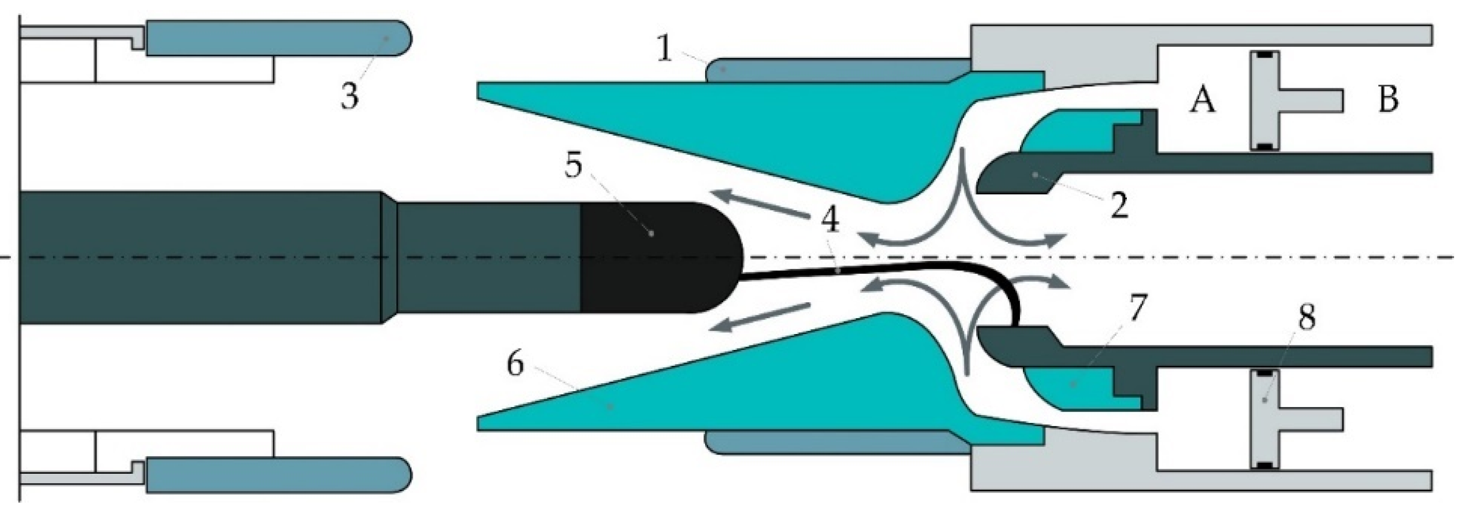
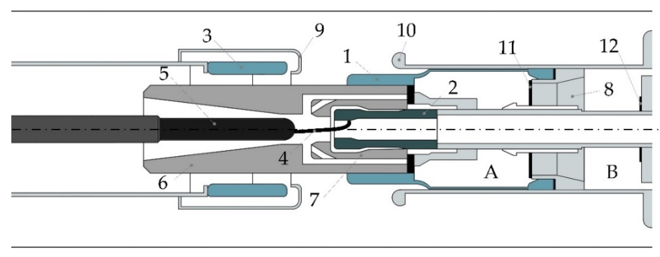
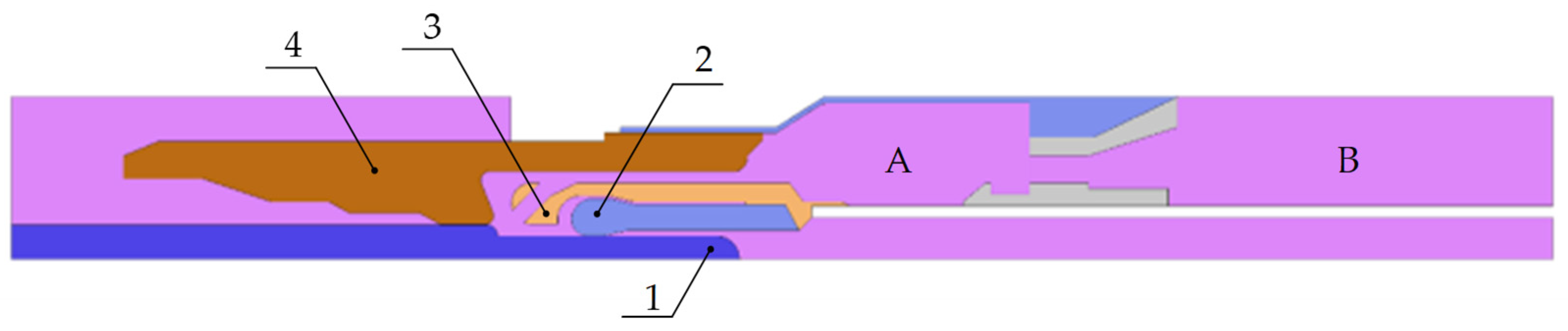
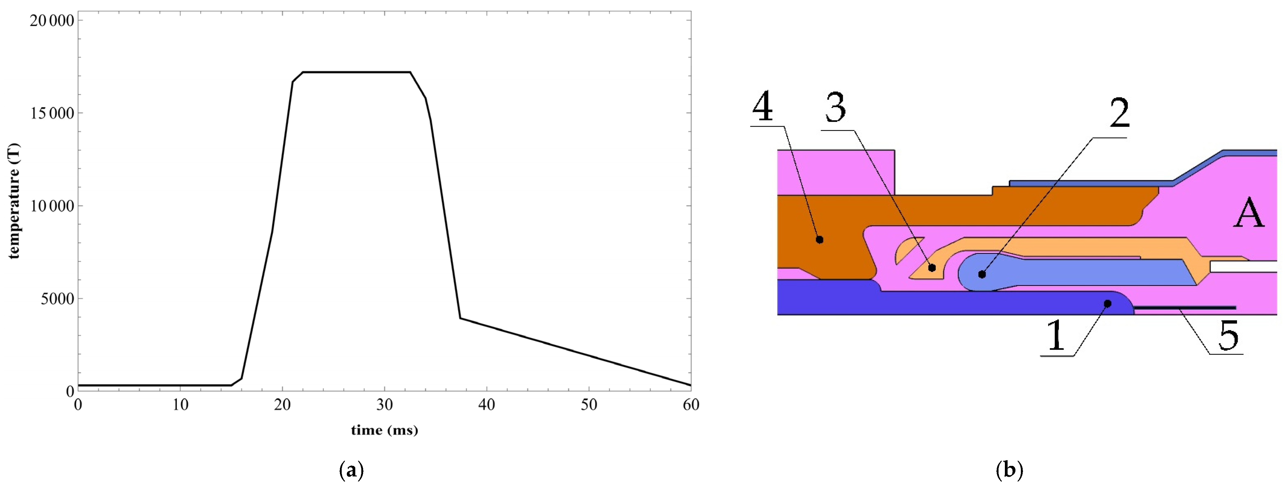
3.1. SF6 Circuit Breaker under Study

Dead-tank SF6 CB for rated voltage 110   kV ( R U ) / 126   kV ( E U ) Figure 5 was chosen as the research object for the calculation of gas-dynamic processes.
The current flow path in the arc extinguisher of the selected CB is conceptually shown in Figure 1: in the closed state, most of the current flows from the live part of the bushing through the tulip contact (is not shown) to the tubes of both the fixed and moving main contacts 9 and 10, passing to the main contacts 1 and 3. When the main contacts open, the current also flows through the tubes 9 and 10 but passes through the conductive parts into the arcing contacts 5 and 7.
Arc extinguishing in the interrupter of this CB is based on combining self-blast and puffer-type principles. The interrupter had PTFE nozzles, providing an additional gas blast when the arc is burning.

3.2. Computational Model of the Circuit Breaker under Study

To calculate the gas dynamics, the following data were required: the full contact separation, the cross section of the piston, as well as the characteristics of the dependence of the cross section of the SF6 gas outlet on the contact separation S = f ( l ) . All these parameters were taken from the approximate geometric dimensions of the tank CB under study:
-
Full contact separation L m a x = 120   m m ;
-
The contact separation before blast start is L e x t = 18   m m ;
-
Piston cross section S p = 8.953   m m 2 ;
-
Ambient medium temperature ϑ = 40   ° C = 313   K ;
-
Pressure inside CB p 0 = 0.42   M p a ;
-
The flow coefficient μ at all stages of the outflow was assumed to be 0.9 (the outflow coefficient, which took into account the decrease in the actual cross section of the hole due to the compression of the jet in it);
-
Adiabatic exponent for SF6 gas k a = 1.086 ;
-
We set the discretization step of the calculation; for this, we divided the entire piston stroke into 20 identical sections: n = 20 . The contact separation in each section would be:
l = L m a x n = 120 20 = 6   m m
Figure 6a,b shows the dependence of the SF6 outlet cross section on the piston stroke S = f ( l ) and the dependence of the piston speed on the contact separation V = f ( l ) for the selected research object— 110   kV SF6 dead-tank CB. The data were taken from the instruction manual of the manufacturer of this CB. Figure 7 shows the contact travel curve, which was taken from [14]. This curve was necessary in numerical implementation when solving a gas-dynamic problem with a moving grid. The total shutdown time was taken as equal to 55 ms.

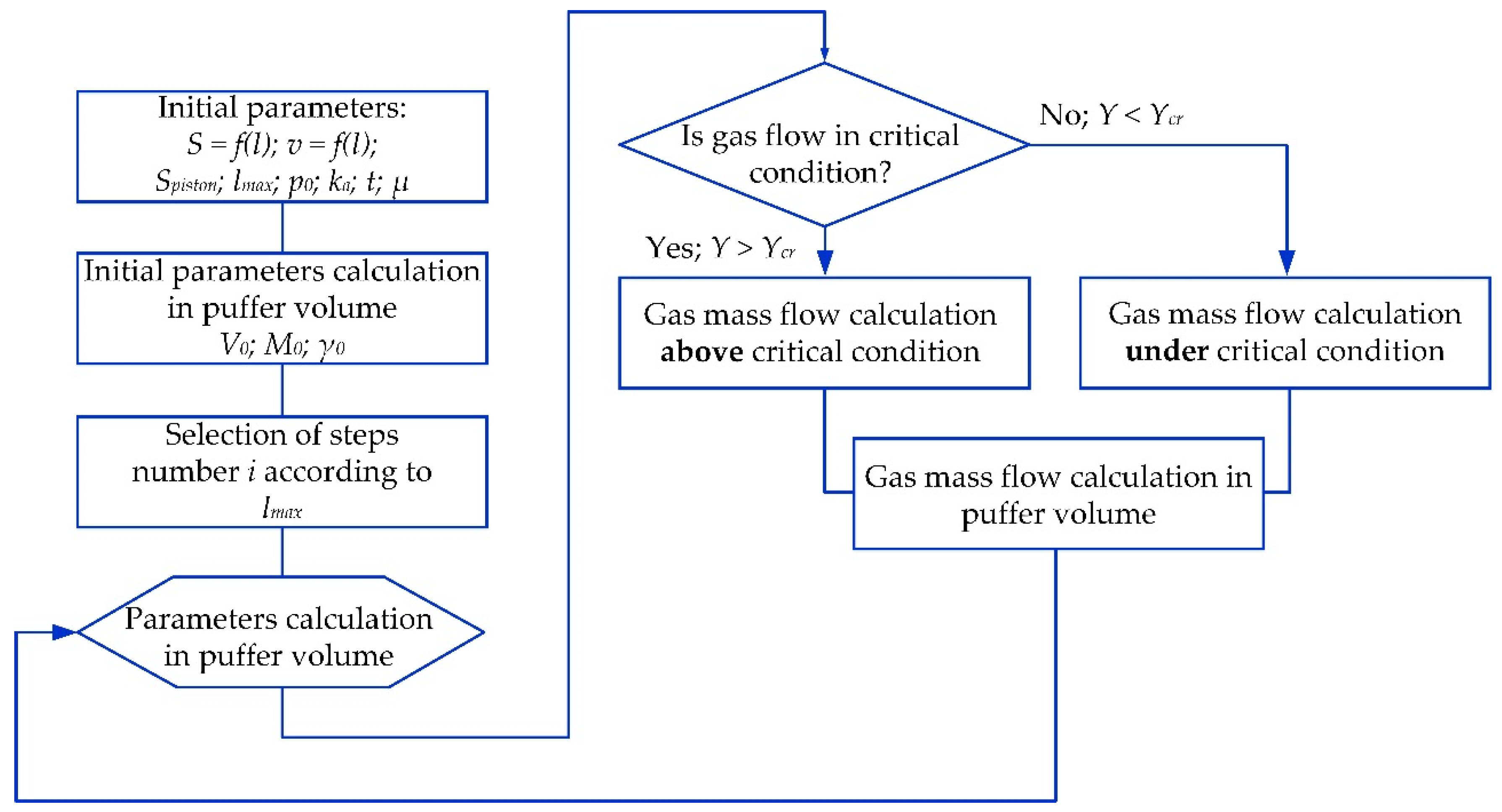
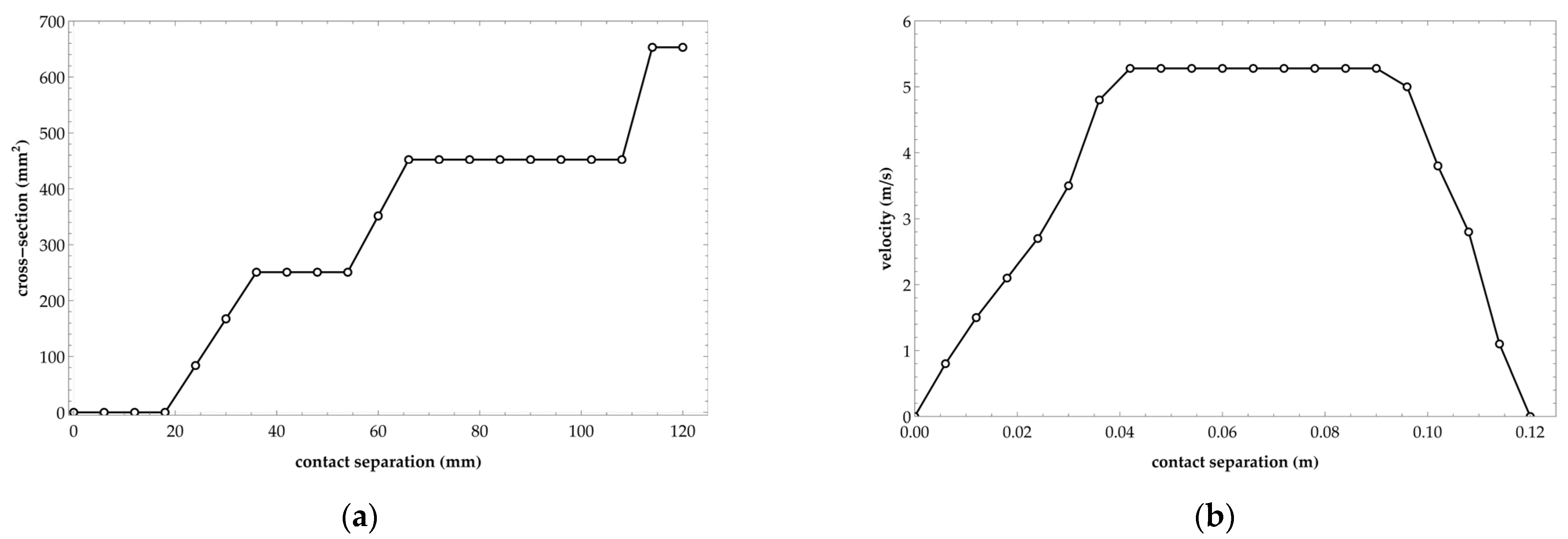
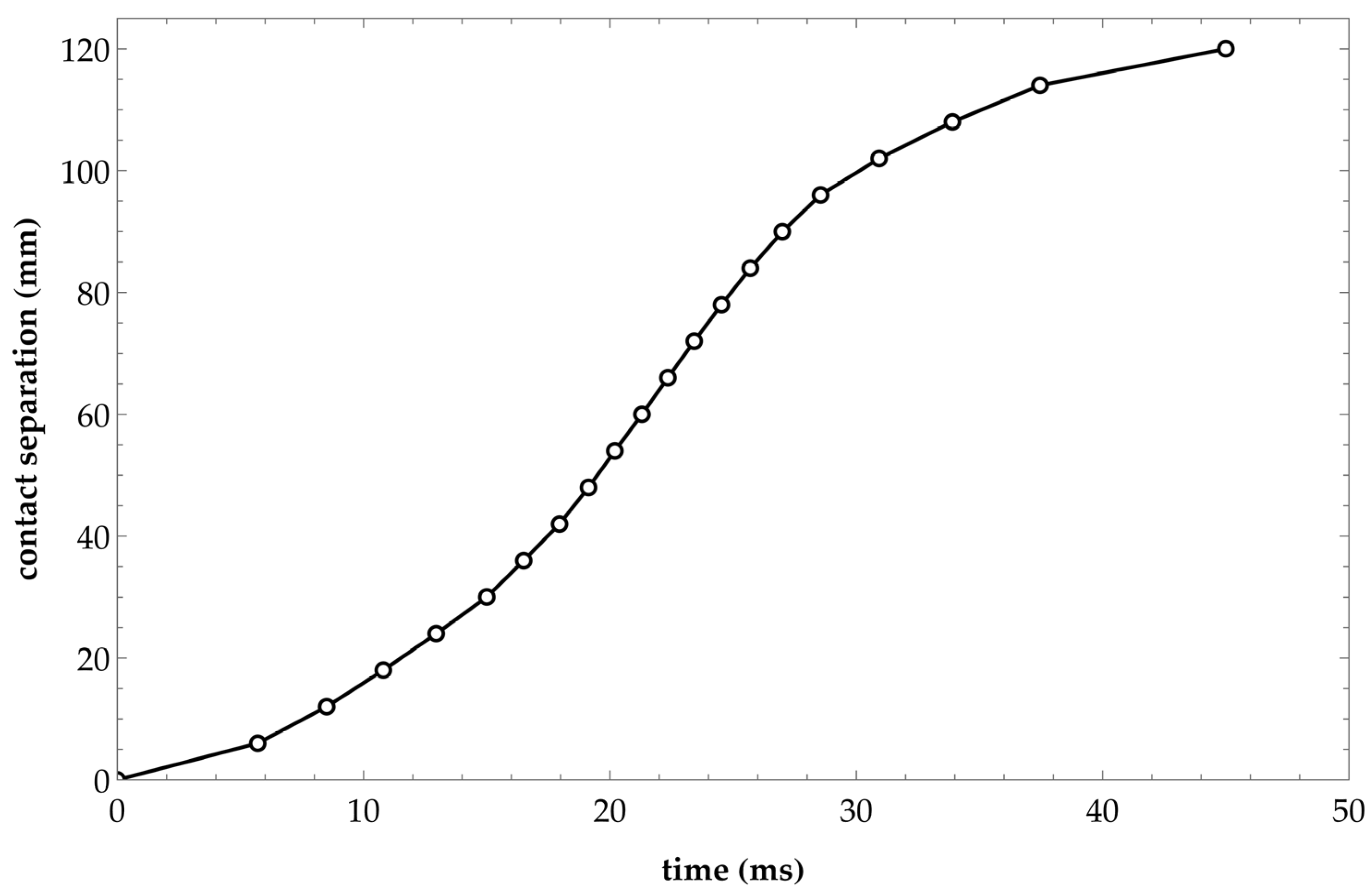
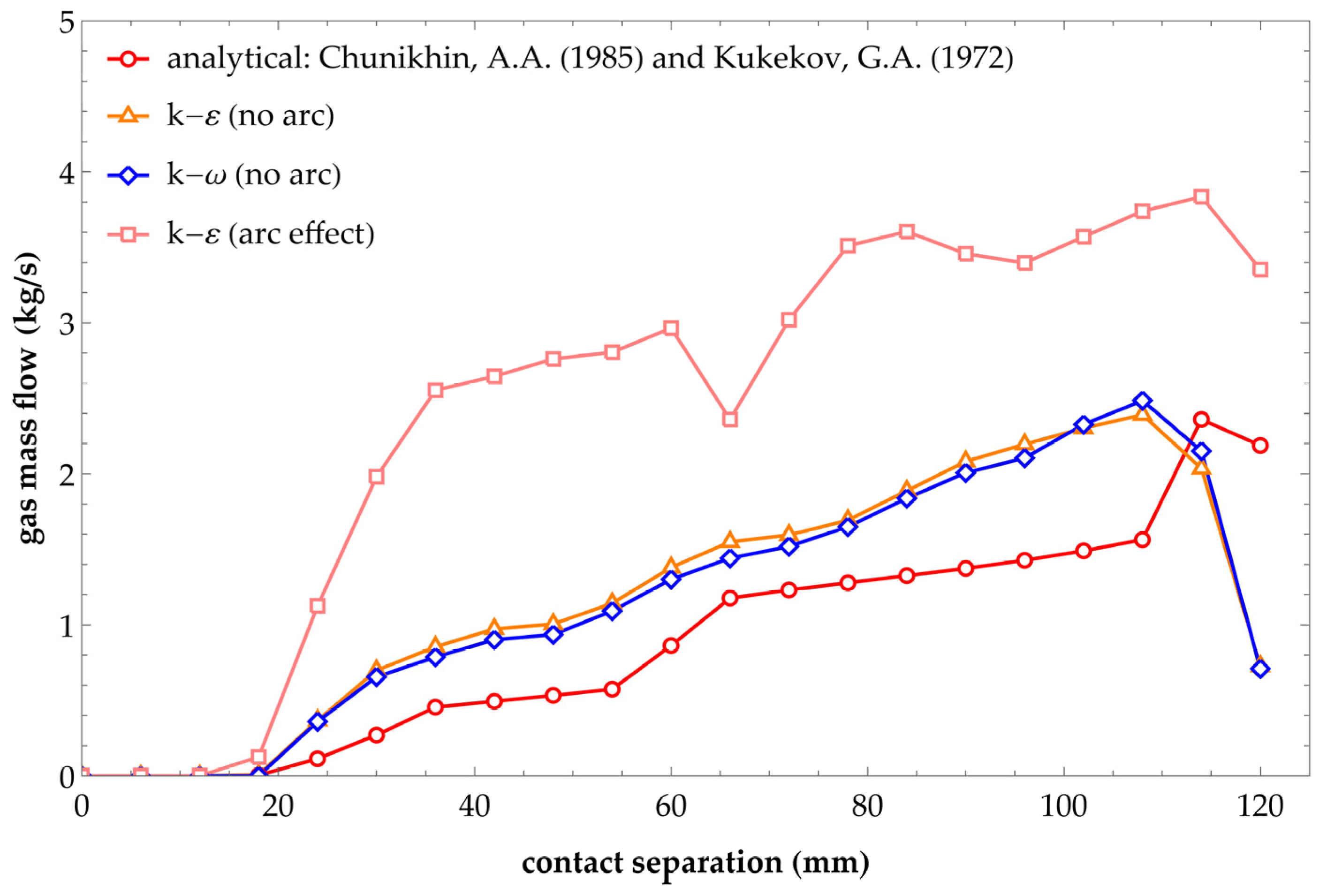
3.3. Calculation Results

The results of the analytical calculation were the pressure changes in the under-piston volume and the mass flow rate per second depending on the contact separation. Table 3 presents the results of calculating each step by the analytical method according to the method [15,18]: pressure in the under-piston volume pi; gas mass flow G i ; mass loss of SF6 during blast; M i ; mass of SF6 gas in the under-piston volume M i ; and relative backpressure Y i . The piston speed vav was taken from Figure 6b. Parameter Ψ Y = 2 k a k a 1 Y 2 k a Y k a + 1 k a characterized the outflow of gas from the volume above the piston for each i calculation step.
Pressure changes in the under-piston volume and mass flow rates depending on the contact separation, plotted according to Table 3 data, are shown in the calculation results in comparison with the numerical calculations.

4. Numerical Calculation of SF6 Gas Circuit Breaker Switching

The analysis was carried out in COMSOL Multiphysics 6.0 software (Academic version) using the finite element method with a moving mesh (ALE).
The Navier–Stokes equations describe nonstationary flows and express momentum balances and mass conservations for a viscid and compressible fluid in the following form [69,70]:
ρ t + · ρ u = 0
where ρ —density; u —flow velocity m/s; and t —time, s.
ρ u t + ρ u · u = p + · μ ( u + u T 2 3 μ ( · u ) I + F
where p —pressure, Pa; F —volume force vector N / m 3 ; and I —turbulence intensity.
The Reynolds number is one of the important criteria in the analysis. The Reynolds number ( R e ) is non-dimensional and describes the ratio between inertial forces and those of viscous friction in viscid fluids and gases.
When the Reynolds number exceeded a boundary value, the precise analytical solution for the dimensional flow or flat plate flow became chaotic, which marked the emergence of the turbulent flow. The Navier–Stokes equations were highly sensitive to changes in coefficient values in the turbulent flow conditions [69,70].
Values of the Reynolds number varied within ( 0.4 10 ) · 10 6 depending on SF6 gas pressure in interruption chamber and geometrical properties of SF6 gas concurrent flow, which blew round the arc [71,72].
There were plenty of various models for turbulent flow analysis. The main idea behind such a model boiled down to the assumption about the existence of average flow velocity and the average deviation from flow velocity. The models that are listed below were used in various engineering applications with different accuracy requirements. Almost all of them have been implemented in modern software for fluid dynamics analysis.
The main models are listed in the order of increasing complexity [67,70]:
-
The Boussinessq model;
-
The Spallart–Allmaras model;
-
The k ε model;
-
The k ω model;
-
The Reynolds stress model;
-
The direct numerical simulation (DNS);
-
The large eddy simulation.
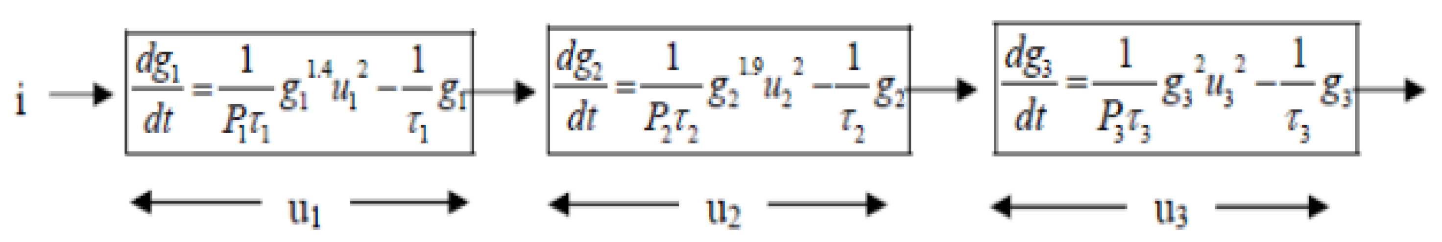
The k ε model was chosen to be used in numerical analysis, with the turbulent flow of gas being taken into account. This model is mainly used in nozzle arc simulations [73,74]. Furthermore, the k ω model was used to simulate CB interruption without arc (no-load mode) due to existence of a boundary layer, which is described below. This model could be efficiently applied in the wall turbulence analysis without additional special functions.

4.1. The k ε Model of Turbulent Flow

The turbulence viscosity ratio μ T for the k ε model is:
μ T = ρ C μ k 2 ε
where ε is velocity of turbulent dissipation, m2/s3; C μ is coefficient of the k ε model; and k is turbulent kinetic energy, m2/s2.
The resultant equations of the k ε model are the following [75]:
The convection–diffusion equation for turbulent kinetic energy k :
ρ k t + ρ u · k = · μ + μ T σ k k + P k ρ ε
The convection–diffusion equation for the dissipation ε :
ρ ε t + ρ u · ε = · μ + μ T σ ε ε + C ε 1 ε k P k C ε 2 ρ ε 2 k
where ε ,   C ε 1 ,   a n d   C ε 2 are model parameters, and their values are listed in Table 4.
The component of deformation rate P k is:
P k = μ T u : u + ( u ) T 2 3 · u 2 2 3 ρ k · u
where « : » means tensor convolution.

4.2. The k ω Model of Turbulent Flow

The turbulence viscosity ratio μ T for the k ω model is:
μ T = ρ k ω
where ω is relative dissipation rate, Hz.
The resultant equations of the k ω model are the following [75]:
The convection–diffusion equation for turbulent kinetic energy k :
ρ k t + ρ u · k = · μ + σ k * μ T k + P k ρ β * k ω
The equation of relative dissipation rate ω :
ρ ω t + ρ u · ω = · μ + σ ω μ T ω + α ω k P k ρ β ω 2
where α ;   β = β 0 f β ;   β * = β 0 * f β ;   σ ω ;   σ k * ;   β 0 ;   f β = 1 + 70 χ ω 1 + 80 χ ω ;   a n d   χ ω = Ω i j Ω j k S k i β 0 * ω 3 —are model parameters, and their values are listed in Table 4.
Ω i j = 1 2 u i x j u j x i is the tensor of average rotation rate;
S i j = 1 2 u i x j u j x i is the tensor of average deformation rate:
Furthermore, the wall boundary conditions were formed for the k ω model [75].

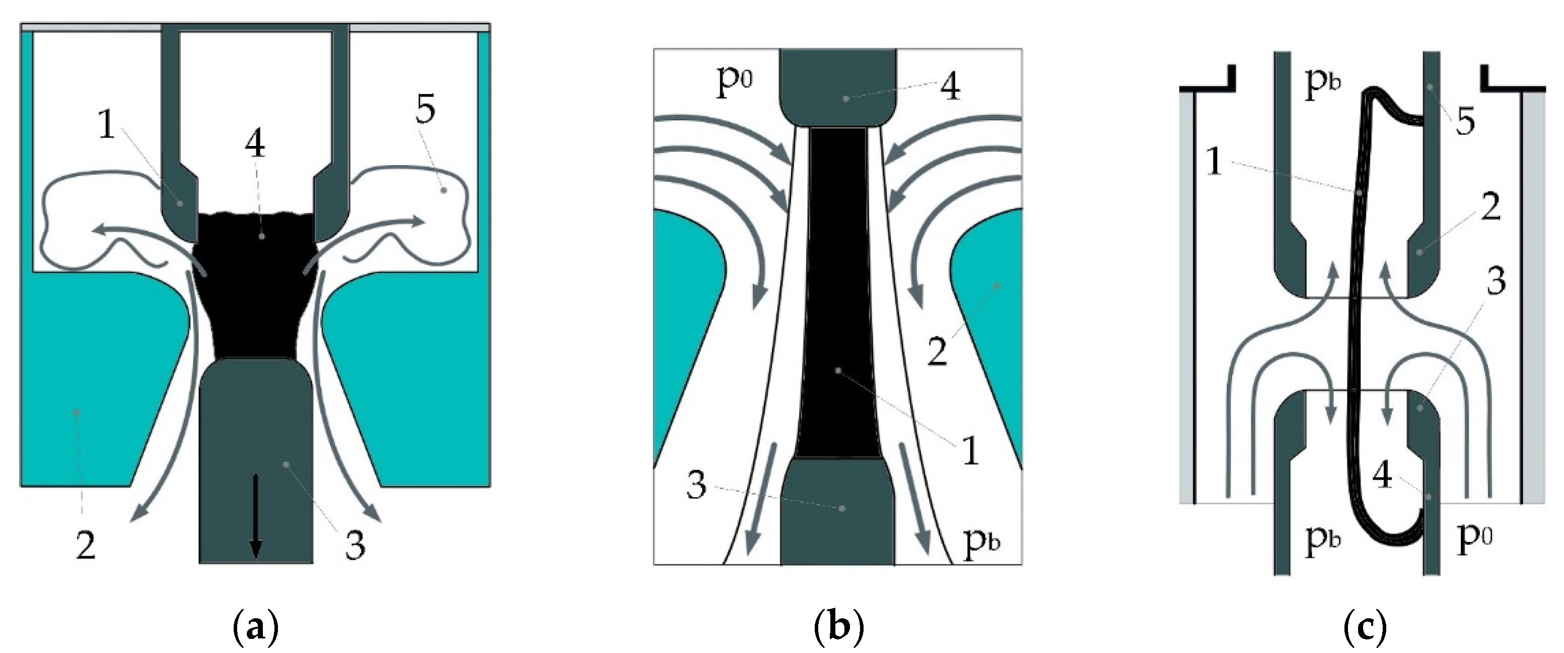
4.3. The Computational Model of the Object under Study

The model of interruption chamber of a dead-tank SF6 gas CB. The dimensions of the model were approximately the same as those of the real CB. Elements of the chamber, which were not utilized in gas dynamics analysis, were not taken into account (Figure 8).
Parameters of the turbulence models k-e and k-w for numerical analysis can be found in Table 4.
The grid of the numerical model was triangular (the triangulation method). The rectangular domain was used at the boundary layer. Grid parameters are shown in Table 5. The calculation was carried out using the finite element method in combination with the arbitrary Lagrangian Eulerian method (ALE). The latter was used to solve gas dynamics equations in the third coordinate system, thus called mesh frame.
This study was distinguished by taking into account the movement of the mobile parts of the object under study in a gas dynamics simulation. The module moving mesh was used to simulate the movement of a piston and the movable contact.
The k-e model included viscous effects that were considered for the sliding wall; consequently, there was a boundary layer. No slip was the default boundary condition to model solid walls. A no-slip wall was a wall where the fluid velocity relative to the wall velocity was zero. For a stationary wall, it meant that u = 0 . The constraint could be mathematically formulated for the problem with a moving wall:
u r e l · n = 0
u r e l = u u t r
K K · n n = 0
K = μ ( u r e l + u r e l T ) n
where n—boundary normal, with direction outside the region; u r e l is relative velocity; and u t r is translation velocity.
Turbulence parameters k and ε were subject to homogenous Neumann boundary conditions:
k · n = 0
ε · n = 0
During the calculation, due to the movement of the boundaries of the object, the grid of the computational domain was strongly deformed, which reduced its quality and led to the appearances of discontinuities, inconvergences of equations, etc. In order to eliminate possible errors, it was customary to use the Automatic Remeshing function, which rebuilt the computational mesh when it reached a critically low quality.

4.4. The Proposed Model of Interaction between SF6 Gas Flow and Arc

The model is based on the additional element, which is either the line (axisymmetric) or cylinder (three-dimensional) in the contact gap. The arc column measured temperature is assigned to the line. The temperature is obtained from the experiment of 10 kA symmetrical short-circuit breaking [76].
The temperature change is shown in Figure 9a. The duration of the application of temperature to the moving line was given with the assumption that the arc burned for two power frequency half cycles (i.e., 20 ms). In this case, it was decided to neglect the change in temperature in the vicinity of the zero current. This assumption was very rough because the problem of skipping current zero was extremely important [77,78,79]. Studies devoted to the analysis of the occurrence of thermal and/or electrical breakdowns due to the passage of zero current gave a complete picture of arcing. However, in this study, the emphasis was on modeling the processes of arcing until the moment of arc extinction, and the processes of restoring electrical strength were not studied.
At the line boundaries (Figure 9b), the temperature of the arc stem was set according to [76] with a current cut of 10 kA. A feature of the model was the fact that the line moved along with the moving contact until the contacts opened (moving mesh). After opening the contacts, the upper point of the line was fixed, and it lengthened after the moving contact. In a three-dimensional picture, this line was represented by a cylindrical arc, on the surface of which the temperature was experimentally set. Thus, gas heating occurs in the contact gap as the contacts are being separated.
When adding heat sources to the model, the heat balance equation was added to the solution of the above equations for gas dynamics:
ρ C p T t + ρ C p u · T + · q = Q + Q p + Q v d ,
where C p is the specific heat capacity at constant pressure, J / ( k g · K ) ;   q —heat flow due to thermal conductivity, W / m 2 ; Q —heat source other than viscous dissipation, W / m 3 ; Q p is the work performed by changing the pressure and is the result of heating during adiabatic compression, as well as some thermoacoustic effects, W / m 3 ; Q v d is viscous dissipation in liquid, W / m 3 .
Q p = α p T p A t + u · p A ,
where α p is the coefficient of thermal expansion, 1 / K :
α p = 1 ρ ρ T p
For heat transport turbulence consideration, the Kays–Crawford model was used (the default in COMSOL Multiphysics). The viscous dissipation, in this case:
Q v d = τ : u + Q t u r b
where τ is the viscous stress tensor, P a .
Heat flux by conduction (RANS turbulence model):
q = ( k + k T ) T
with the turbulent thermal conductivity defined as:
k T = μ T C p P r T
where P r T —Prandtl number, according to [80].
In this case, the boundary conditions for the first kind of Dirichlet were written in the form of Equations (41) and (42) on the boundary where there was no heat flux across the boundary (in general form):
n · q = 0
However, taking the wall treatment into account, the boundary condition is rewritten as:
n · q = q w f = ρ C p u τ T w T T +
where q w f —the heat flux between the fluid with temperature T and a wall with temperature T w ; C p —is the fluid heat capacity; u τ —is the friction velocity given by wall treatment (Equations (29)–(32)); T w —wall temperature (on the boundaries which are “temperature source”); and T + – is the dimensionless temperature and is given by [81].
The temperature on the boundaries that represent the experimental arc temperature profile (according to [76]):
T = T 0

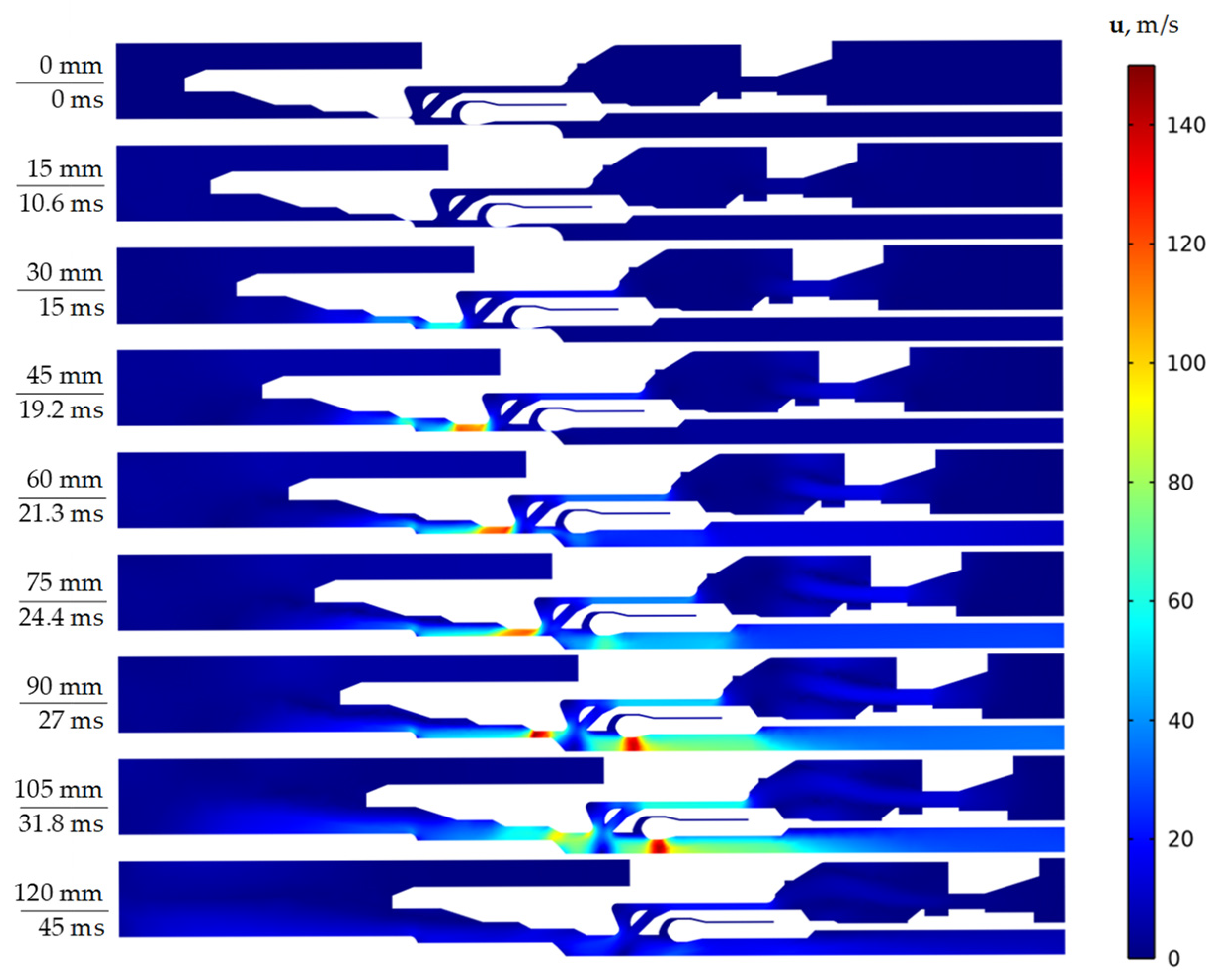
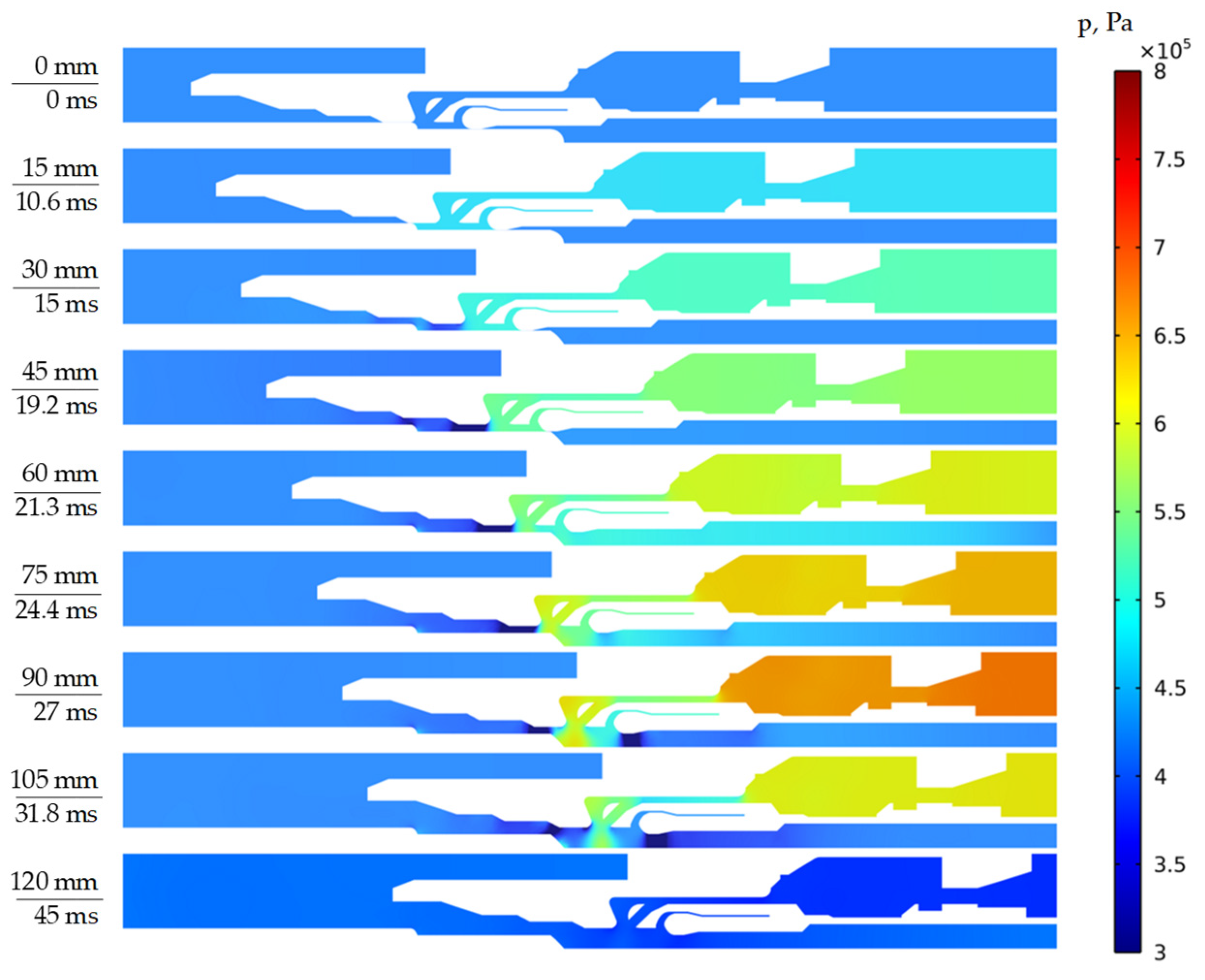
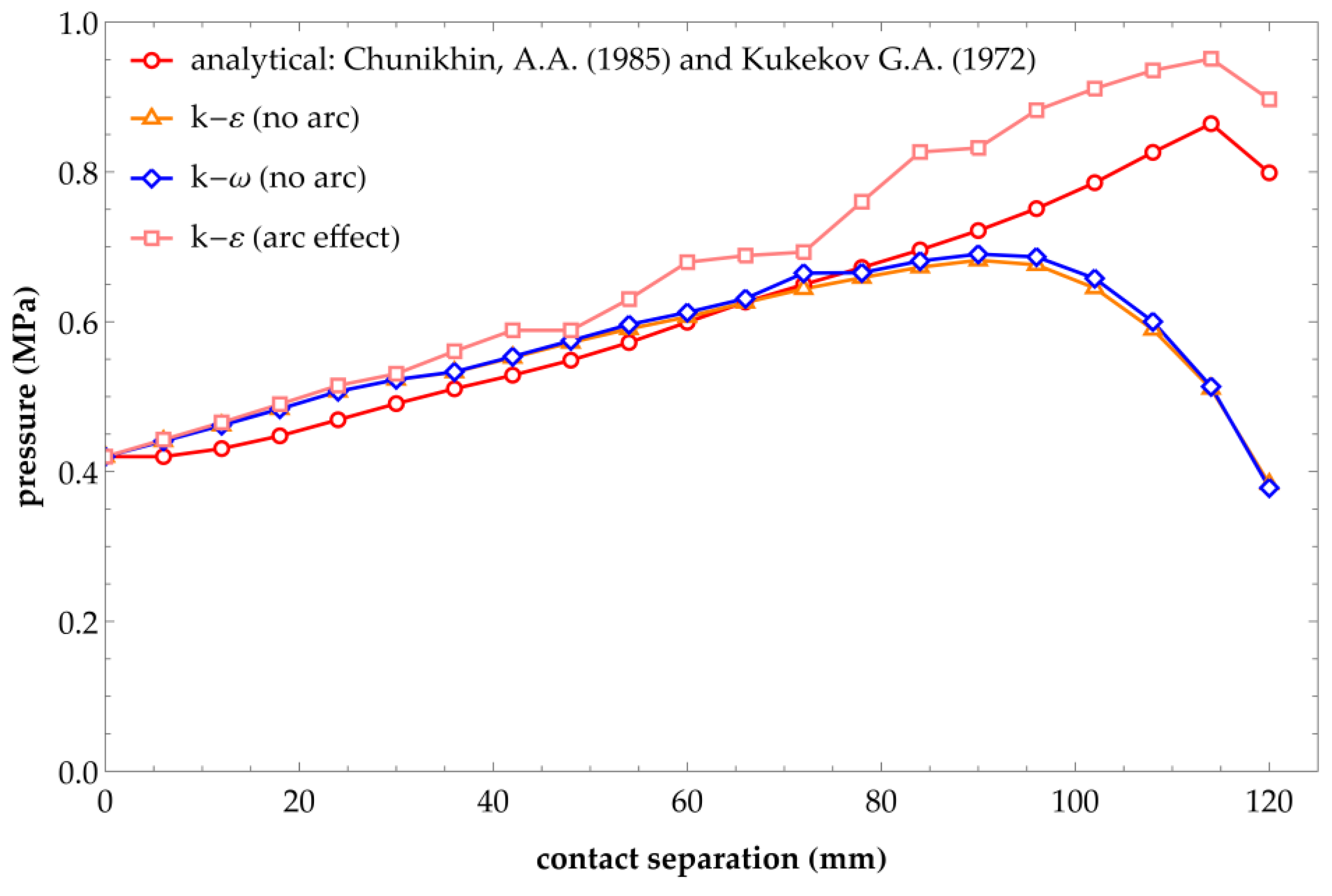
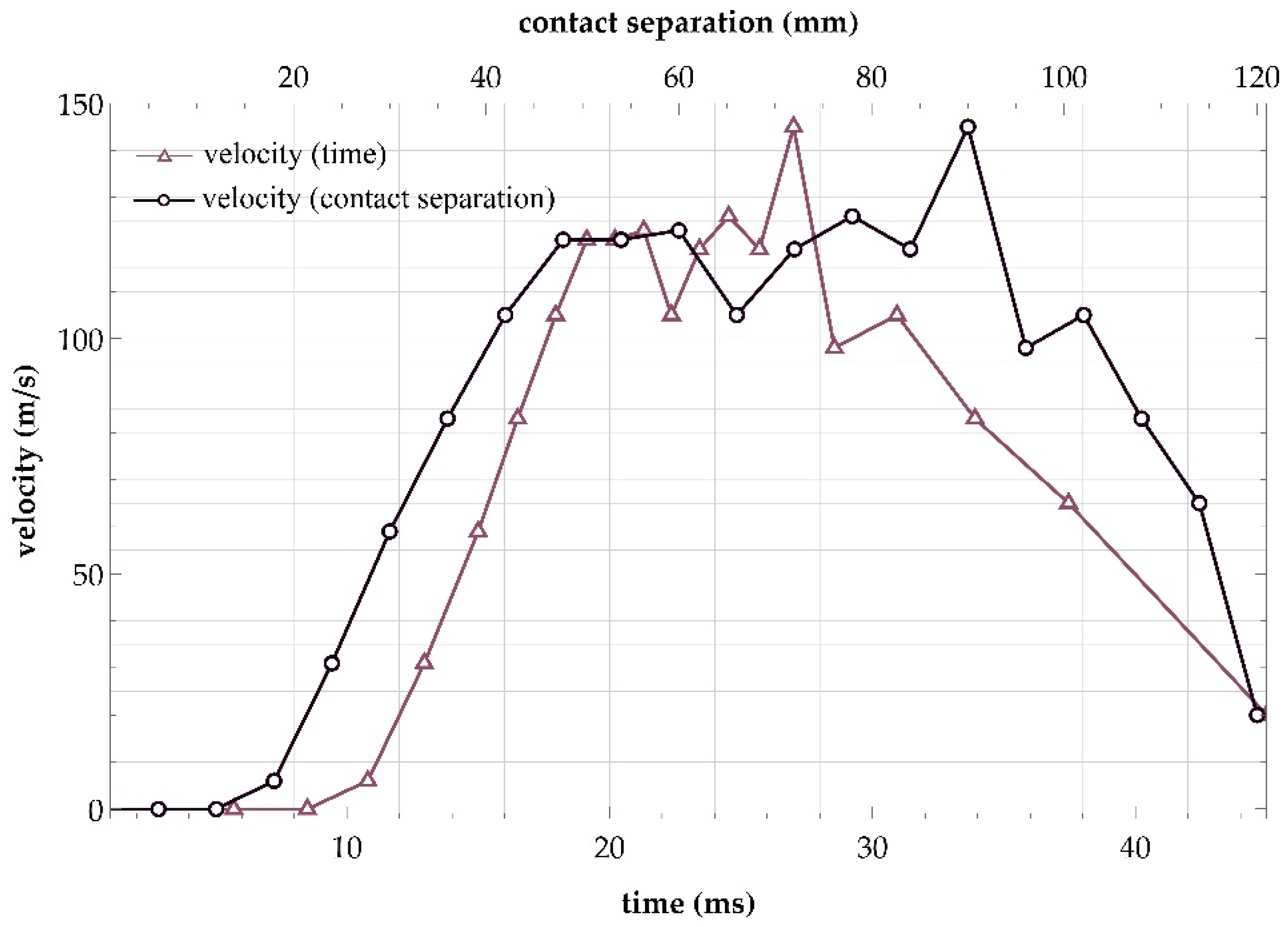
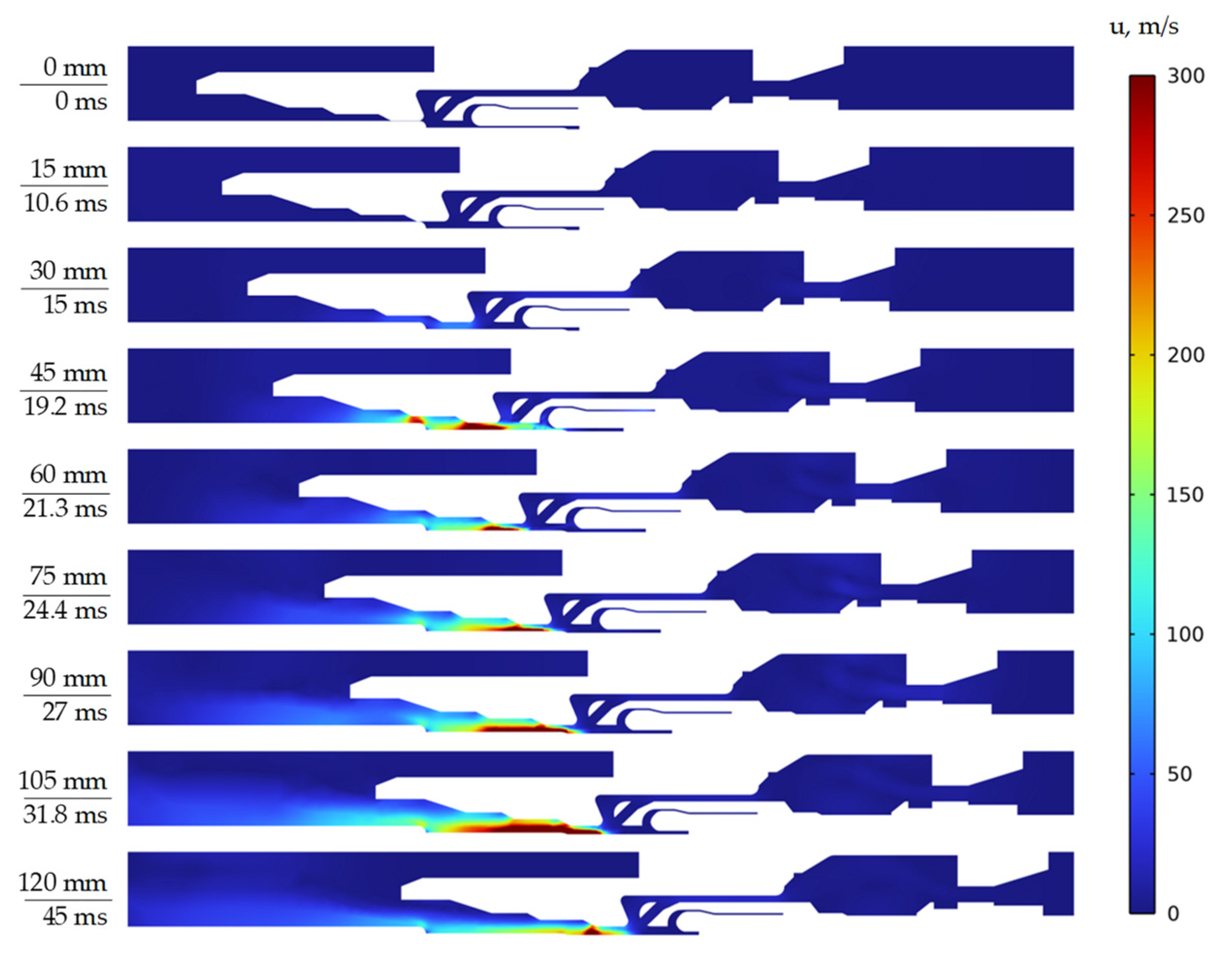
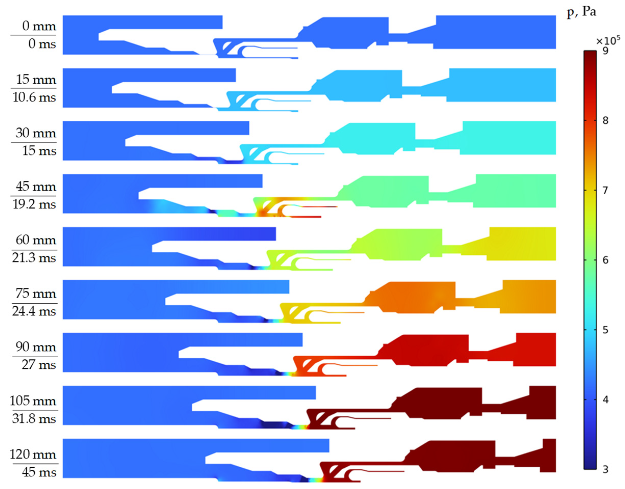
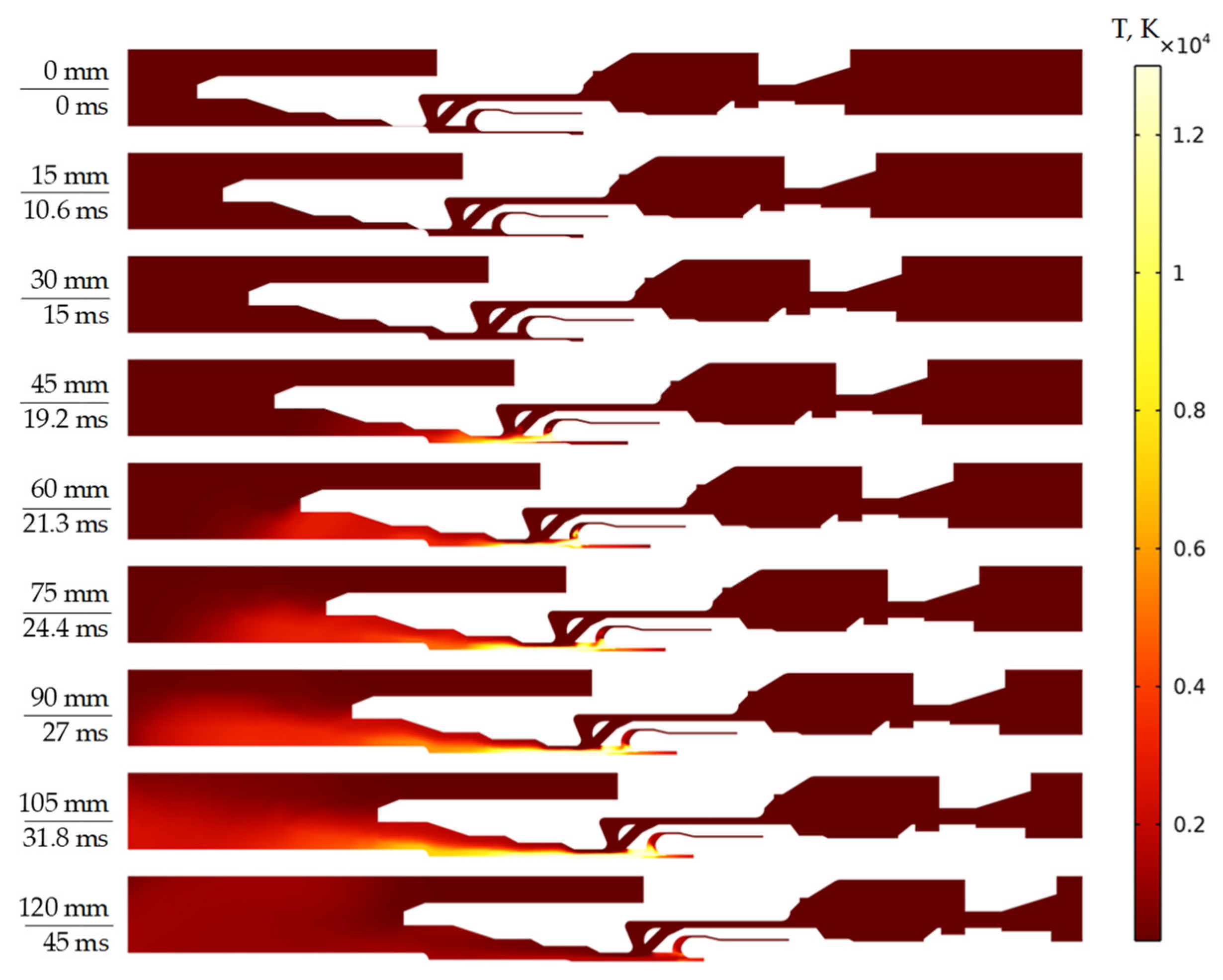
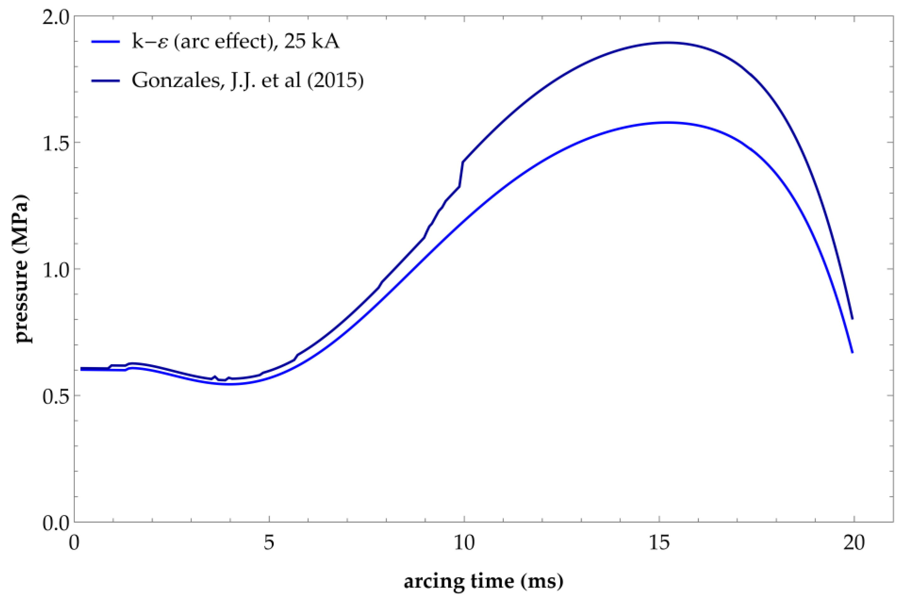
4.5. Calculation Results

Table 6 presents the results of calculation of two turbulent models ( k ε and k ω ) of the main gas-dynamic parameters: pressure in the under-piston volume p ; gas velocity in the nozzle u ; mass flow rate G . For convenience, all results are given to contact separation, which are considered in the analytical calculation.
Furthermore, the results of the calculations are presented in the form of fields of profiles of speeds, pressures, and temperatures, as the contact system of the arcing device moved when the short circuit currents were turned off. In the profile field, the gas and the corresponding changes in dependent variables (gas velocity, pressure, temperature) are shown in color, and the solid elements of the arc extinguisher involved in the movement (nozzles, contacts, pre-piston areas) are shown in white.
Figure 10 shows the fields of velocity profiles for different positions of the moving part without taking into account the arc (turbulence model k ε ). It can be seen that the gas velocity inside the moving contact cavity exceeded the gas velocity in the nozzle at some moments. However, even in this case, the main volume of gas flowed out through a large nozzle because the cross-sectional area of the nozzle was greater than the cross-sectional area inside the moving contact.
Figure 11 shows the change in gas pressure at different positions of the moving part without taking into account the arc (turbulence model k ε ). An increase in the pressure in the under-piston and above-piston volumes could be noticed (assumption: it was assumed that there is no valve between them). With a real shutdown of the short-circuit current, the valve between the areas would begin to close, and the arc extinguishing was mainly carried out by blowing from the above-piston volume. Furthermore, the figure basically shows that the pressure in the contact gap was pumped after the opening of the large nozzle (contact separation is 90 mm).
Figure 12 shows the change in pressure in the under-piston volume for both analytical and the numerical calculations, taking into account the turbulent models k ε and k ω , respectively. According to Figure 12, it can be seen that the pressure in the under-piston volume changed smoothly—almost linearly almost until the very end of the contact separation. This happened due to the neglect of both turbulent SF6 gas flows and the impact of the shutdown arc on this flow. According to the results obtained numerically, it is seen that the pressure peak occurred at the moment of the deceleration of the contact separation, which was t = 27   m s . The decrease in pressure could be explained by the fact that the gas compression rate slowed down, whereas the mass flow continued to increase.
Figure 13 shows the gas mass flow change through the section of the under-piston volume. It can be seen that the flow curve was tied to the cross section of the regions that the SF6 gas passed on the way to the contact gap, as in the analytical calculation. The differences were caused by less linear transitions with an increase in the cross-sectional area of the SF6 gas movement in the direction of the contact system due to turbulence. This meant that the analytical method gave only a superficial understanding of gas dynamics during the CB breaking or making. Considering the turbulent flows (without arc affect) and turbulent heat transport (with arc affect), even with low relative tolerance, gave a different nature of the interrupter’s switching process. The proposed numerical model might have been used for the influence estimation of the thermal effect of the switching arc on the nozzles, as well as for the estimation of both the thermal and electric breakdowns.
Figure 14 shows the gas velocity change in the narrowest part of the nozzle (confuser) versus time and contact separation, respectively.
Up to a certain point in time ( t c r i t = 19.13   ms ), the gas velocity increased, after which some constancy could be observed. Therefore, we could assume that the speed had reached its critical value. This meant that the time t c r i t could be considered a critical point, and the time interval up to this point was a subcritical gas outflow regime. The interval after the critical point and before the moment of braking was a supercritical regime of gas outflow. Velocity fluctuations occurred due to additional outflow of gas into the area of the opened section inside the moving contact.
Figure 15 shows the gas velocity field, taking into account the setting of the arc in the form of a thermal heating source. It can be seen that the gas velocity during opening reached supersonic values (the speed of sound in SF6 gas under normal conditions was 130 135   m / s and increased with increasing pressure of the medium). For the process of arc extinguishing, this was a favorable factor because there was an intensification in the cooling of the plasma channel of the cut-off arc. However, one could also notice that a local area was formed along the stationary arcing contact, where the velocities prevailed. This fact was due to the assumption made in the calculation model—the main part of the arc-extinguishing movable contact was cut out. Thus, it was considered that the main blast was directed through a large nozzle (disconnection of high short-circuit currents).
Figure 16 shows the gas pressure field, taking into account the setting of the arc in the form of a thermal heating source. When such a short-circuit current breaking took place, the pressure increased by about 2.0 2.5 times from the nominal value ( 0.5   MPa ) and reached approximately 1.0 1.5   MPa for the self-blast-type interrupters [17].
Figure 17 shows a picture of the temperature profile in the arc quencher during shutdown. In contrast to the arc-free mode, there was a clear change in the SF6 flow in the contact gap due to the occurrence of flow stagnation areas, where the SF6 gas flow, passing through a small nozzle, met the SF6 gas flow going through a large nozzle. However, their directions were opposite to each other. The local heating of the area along the fixed arcing contact was due to the assumption made above.
Due to the consideration of the arc action, the pressure in the contact gap changed and has a less decreasing character, in contrast to the arc-free mode.

5. Conclusions

In the developed model described above, the temperature characteristics of the arc shaft were obtained from the experiment of switching off the symmetrical short-circuit current of 10 kA [76]. The proposed model of the switching arc was implemented in numerical software using the finite element method based on a moving-mesh technique (ALE method). The ALE method allowed us to take the contact separation curve of the CB into consideration and to make the developed model adaptive. In order to make a comparison with experimental data on breaking higher short-circuit currents, the temperature change was adapted according to [73] for an arcing time of 20 ms (two half cycles of power frequency). The accuracy of the developed model was determined in comparison with experiments on breaking the symmetrical current of 25 kA by a self-blast interrupter from the study [82]. The comparison was carried out by the means of calculating the coefficient of determination R 2 by changing the pressure in the under-piston volume (Figure 18). Due to the consideration of the arc effect, the pressure in the contact gap changed and had a less decreasing character, in contrast to the arc-free case.
From Figure 18, it can be seen that the developed model in the form of a temperature heating source had a good quality in comparison with the experiment [82], with a determination coefficient R 2 = 0.997 .
According to the results of the calculations, it is advisable to note the assumptions and critical parameters of the model:
1. The absence of a valve between the under-piston and above-piston volumes, which clearly affects the velocity profile of the SF6 flow moving into the contact gap.
2. Cut out the main part of the arcing moving contact, leading to a one-way blow (through a large nozzle). Therefore, the model was suitable for breaking large short-circuit currents.
3. The construction of the computational grid was performed by the user (user controlled) and not by the built-in tools of the numerical software complex (physics controlled). As a result, the computational mesh on the boundary layers had the same quality as in the main computational domain. In other words, the calculation of gas dynamics was carried out quite roughly.
4. The buoyancy forces were not taken into account in the calculations of gas dynamics.
5. The assumption of Mach numbers <0.3 was used. However, in the peak phases of the arcing, the SF6 flow velocity exceeded the supersonic flow. Thus, it was more correct to use models that were used for the sonic and supersonic flows’ descriptions.
6. To increase the convergence, the accuracy parameter of the moving grid (relative tolerance) was taken as equal to 0.1, which made it possible to consider the physical processes only in the first approximation.
7. The contact separation curve was taken from the arc-free case (“no-load”) and was considered unchanged even when the arc was taken into account. However, when the arc was extinguished, the contact separation curve “collapses” [83], which clearly affected the entire process of the gas dynamics, including the gas outflow regime.
8. Despite the fact that the radiation effect was significant within such high temperatures of the switching arc column (>13,000 K), the assumption of the neglecting this effect was used.
As prospects for further research directions, in addition to considering the above assumptions, the following can be noted:
1. Taking all the physical processes of interaction the SF6 gas flow and switching arc (creation of magnetohydrodynamic, hydrokinetic, and kinetic models that make it possible to trace the movement of the conductive medium—the arc plasma in SF6 gas), with the aim of their possible syntheses and the creation of universal approaches to the simulation of the switching arc.
2. Adapt the developed model for “near zero” arc extinguishing processes, taking into account the processes of restoring the electrical strength of the contact gap, the residual conductivity of the arc, and assessing the likelihood of thermal and electrical breakdowns, etc.
3. An improvement of the methods for calculating the equations of gas dynamics in order to minimize computational costs.
4. Analyze the occurrence of computational instability in the calculations of gas dynamics and develop prerequisites for combating this problem without losing the accuracy of the simulation.

Author Contributions

Conceptualization, V.V.P., A.I.K. and Y.V.P.; methodology, A.I.K. and V.V.P.; software, V.V.P. and Y.V.P.; validation, A.I.K. and V.V.P.; writing—original draft preparation, A.I.K., V.V.P. and Y.V.P.; writing—review and editing, A.I.K. and V.V.P.; visualization, V.V.P.; supervision, A.I.K. All authors have read and agreed to the published version of the manuscript.

Funding

The research was carried out within the state assignment with the financial support of the Ministry of Science and Higher Education of the Russian Federation (subject No. FEUZ-2022-0030 Development of an intelligent multi-agent system for modeling deeply integrated technological systems in the power industry).

Conflicts of Interest

The authors declare no conflict of interest.

References

  1. Küchler, A. High Voltage Engineering. Fundamentals—Technology—Applications; Springer-Verlag GmbH Germany: Schweinfurt, Germany, 2018; 650p. [Google Scholar] [CrossRef]
  2. GOST 52565-2006; Alternating-Current Circuit Breakers for Voltages from 3 to 750 kV. General Specifications. National standard of Russia. Rosstandart: Moscow, Russia, 2007; 91p. (In Russian)
  3. IEC 62271-100; High-Voltage Switchgear and Controlgear—Part 100: Alternating-Current Circuit-Breakers. IEC: Geneva, Switzerland, 2008; 695p.
  4. IEC 62271-110; High Voltage Switchgear and Controlgear—Part 110: Inductive Load Switching, Ed. 2.0. IEC: Geneva, Switzerland, 2017; 60p.
  5. IEEE Std C37.015–2017 (Revision of IEEE Std C37.015-2009); Guide for the Application of Shunt Reactor Switching. IEEE: New York, NY, USA, 2018; 62p. [CrossRef]
  6. Zalesskiy, A. Electric Arc; Gosenergoizdat: Leningrad, Russia, 1963; 267p. (In Russian) [Google Scholar]
  7. Engelsht, V.; Gurovich, V.; Desyatkov, G. Electric Arc Column Theory; AN USSR, Siberian department, Thermal physics institute: Novosibirsk, Russia, 1990; 373p. (In Russian) [Google Scholar]
  8. Agafonov, G.; Babkin, I. High Voltage Electrical Apparatus with SF6 Insulation; Energoatomizdat: St. Petersburg, Russia, 2002; 728p. (In Russian) [Google Scholar]
  9. Tonkonogov, E. The Design of Electrical Apparatus. High Voltage SF6 Circuit Breakers; Izdatelstvo of Peter the Great St. Petersburg Polytechnic University: St. Petersburg, Russia, 2008; 160p. (In Russian) [Google Scholar]
  10. Averyanova, S.A. Theory of Arc Extinguishing in Electrical Apparatuses. Interaction of the Electric Arc with the Gas Flow in High Voltage Circuit Breakers; Izdatelstvo of Peter the Great St. Petersburg Polytechnic University: St. Petersburg, Russia, 2015; 68p. (In Russian) [Google Scholar]
  11. Poltev, A. Design and Calculation of SF6 High Voltage Apparatus; Energiya, Leningrad department: Leningrad, Russia, 1979; 240p. (In Russian) [Google Scholar]
  12. Eroshenko, S. Calculation of Short Circuit Currents in Power Systems; Izdatelstvo of Ural Federal University: Ekaterinburg, Russia, 2019; 104p. (In Russian) [Google Scholar]
  13. Khalyasmaa, A.I.; Eroshenko, S.A.; Zinovyev, K.A.; Bolgov, V. Improvement of Short-Circuit Calculation Results Reliability for Large Electric Power Systems. In 2019 Electric Power Quality and Supply Reliability Conference and 2019 Symposium on Electrical Engineering and Mechatronics, PQ and SEEM 2019; IEEE: Kärdla, Estonia, 2019; pp. 1–6. [Google Scholar] [CrossRef]
  14. Il’in, A.S. Mathematical Modeling of Thermodynamic Processes of Arc Extinguishing in SF6 flow in Electrical Apparatus; Candidate of Technical Science Dissertation, Ural Federal University: Ekaterinburg, Russia, 2012. (In Russian) [Google Scholar]
  15. Chunikhin, A.; Zhavoronkov, M. High Voltage Apparatus; Energoatomizdat: Moscow, Russia, 1985; 432p. (In Russian) [Google Scholar]
  16. Smeets, R.; Van Der Sluis, L.; Kapetanović, M.; Peelo, D.; Janssen, A. Switching in Electrical Transmission and Distribution Systems, 1st ed.; John Wiley & Sons, Ltd.: Chichester, UK, 2015; 425p. [Google Scholar]
  17. Kapetanović, M. High Voltage Circuit Breakers; Faculty Electrotech. Eng., Univ. Sarajevo: Sarajevo, Bosnia and Herzegovina, 2011; 648p. [Google Scholar]
  18. Kukekov, G. High Voltage AC Circuit Breakers, 2nd ed.; revised; Energiya, Leningrad Department: Leningrad, Russia, 1972; 336p. (In Russian) [Google Scholar]
  19. Cassie, A.M. A new theory of rupture and circuit severity. CIGRE Rep. 1939, 102, 588–608. [Google Scholar]
  20. Mayr, O. Beitrage zur Theorie des Statischen und des Dynamischen Lichtbogens. Arch. Für Elektrotechnik 1943, 37, 588–608. (In German) [Google Scholar] [CrossRef]
  21. Browne, T.E. A study of A-C. arc behavior near currents zero by means of mathematical models. AIEE Trans. 1948, 67, 147–153. [Google Scholar] [CrossRef]
  22. Browne, T.E. An Approach to Mathematical Analysis of A-C Arc Extinction in Circuit Breakers. AIEE Trans. 1959, 77, 1508–1517. [Google Scholar] [CrossRef]
  23. Ragaller, K. Current Interruption in High-Voltage Networks, 1st ed.; Springer: New York, NY, USA, 1978; 360p. [Google Scholar] [CrossRef]
  24. Hermann, W.; Kogelschatz, U.; Niemeyer, L.; Ragaller, K.; Schade, E. Experimental and theoretical study of a stationary high-current arc in a supersonic nozzle flow. J. Phys. D (Appl. Phys.) 1974, 7, 1703–1723. [Google Scholar] [CrossRef]
  25. Hermann, W.; Ragaller, K. Theoretical description of the current interruption in HV gas blast breakers. IEEE Trans. Power Appar. Syst. 1977, 96, 1546–1555. [Google Scholar] [CrossRef]
  26. Tuma, D.T.; Lowke, J.J. Prediction of properties of arcs stabilized by forced convection. J. Appl. Phys. 1975, 46, 3361–3367. [Google Scholar] [CrossRef]
  27. Lowke, J.J.; Ludwig, H.C. A simple model for high-current arcs stabilized by forced convection. J. Appl. Phys. 1975, 46, 3352–3360. [Google Scholar] [CrossRef]
  28. EI-Akkari, F.R.; Tuma, D.T. Simulation of transient and zero current behavior of arcs stabilized by forced convection. IEEE Trans. Power Appar. Syst. 1977, 96, 1784–1788. [Google Scholar] [CrossRef]
  29. Swanson, B.W. Nozzle arc interruption in supersonic flow. IEEE Trans. Power Appar. Syst. 1977, 96, 1697–1706. [Google Scholar] [CrossRef]
  30. Il’in, A.S. Numerical simulation of arc quenching processes in a high-voltage SF6 circuit breaker and comparison of results with real tests. Sci. Tech. Bull. Povolzhye 2011, 5, 140–146. (In Russian) [Google Scholar]
  31. Il’in, A.S. Model of arc quenching processes in high voltage circuit breaker. Electrotekhnika 2011, 12, 36–42. (In Russian) [Google Scholar]
  32. Park, S.H.; Kim, H.K.; Bae, C.Y.; Jung, H.K. Evaluation on Short Line Fault Breaking Performance of SF6 Gas Circuit Breaker Considering Effects of Ablated Nozzle Vapor. IEEE Trans. Magn. 2009, 45, 1836–1839. [Google Scholar] [CrossRef]
  33. Park, J.H.; Kim, K.H.; Yeo, C.H.; Kim, H.K. CFD Analysis of Arc-Flow Interaction in a High-Voltage Gas Circuit Breaker Using an Overset Method. IEEE Trans. Plasma Sci. 2014, 42, 175–184. [Google Scholar] [CrossRef]
  34. Schavemaker, P.H.; Van Der Sluis, L. An Improved Mayr-Type Arc Model Based on Current-Zero Measurements. IEEE Trans. Power Deliv. 2000, 15, 580–584. [Google Scholar] [CrossRef] [Green Version]
  35. Smeets, R.P.P.; Kertész, V. Evaluation of High-Voltage Circuit Breaker Performance with a Validated Arc Model. IEEE Proc. Gener. Transm. Distrib. 2000, 147, 121–125. [Google Scholar] [CrossRef] [Green Version]
  36. Ahmethodžić, A.; Kapetanović, M.; Sokolija, K.; Smeets, R.P.P.; Kertész, V. Linking a Physical Arc Model with a Black Box Arc Model and Verification. IEEE Trans. Dielectr. Electr. Insul. 2011, 18, 1029–1037. [Google Scholar] [CrossRef]
  37. Ohtaka, T.; Kertesz, V.; Smeets, R.P.P. Novel Black-Box Arc Model Validated by High-Voltage Circuit Breaker Testing. IEEE Trans. Power Deliv. 2018, 33, 1835–1844. [Google Scholar] [CrossRef]
  38. Sinkevich, O.A.; Stahanov, I.P. Plasma Physics. Stationary Processes in a Partially Ionized Gas; Graduate school: Moscow, Russia, 1991; 191p. (In Russian) [Google Scholar]
  39. Cherednichenko, V.S.; Anshakov, A.S.; Kuzmin, M.G. Plasma Electrotechnological Installations; Izdatelstvo of Novosibirsk State University: Novosibirsk, Russia, 2009; 508p. (In Russian) [Google Scholar]
  40. Boulos, M.I.; Fauchais, P.L.; Pfender, E. Handbook of Thermal Plasmas; Springer: Cham, Switzerland, 2020; p. 1500. [Google Scholar] [CrossRef]
  41. Zhong, L.; Cressault, Y.; Teulet, P. Evaluation of Arc Quenching Ability for a Gas by Combining 1-D Hydrokinetic Modeling and Boltzmann Equation Analysis. IEEE Trans. Plasma Sci. 2019, 47, 1835–1840. [Google Scholar] [CrossRef]
  42. Zhong, L.; Gu, Q.; Zheng, S. An Improved Method for Fast Evaluating Arc Quenching Performance of a Gas Based on 1D Arc Decaying Model. Phys. Plasmas. 2019, 26, 103507. [Google Scholar] [CrossRef]
  43. Zhong, L.; Wang, J.; Wang, X.; Rong, M. Comparison of Dielectric Breakdown Properties for Different Carbon-Fluoride Insulating Gases as SF6 Alternatives. AIP Adv. 2018, 8, 085122. [Google Scholar] [CrossRef] [Green Version]
  44. Ivanov, M.F.; Galburt, V.A. Numerical Simulation of Gas and Plasma Dynamics by Particle Methods; Izdatelstvo of Moscow Institute of Physics and Technology: Moscow, Russia, 2000; 168p. (In Russian) [Google Scholar]
  45. Klimontonovich, Y.L. Kinetic Theory of Non-Ideal Gas and Non-Ideal Plasma; Science: Moscow, Russia, 1975; 352p. (In Russian) [Google Scholar]
  46. Fridman, A.; Kennedy, L.A. Plasma Physics and Engineering, 3rd ed.; CRC Press: Boca Raton, FL, USA, 2021; 724p. [Google Scholar] [CrossRef]
  47. Muratović, M.; Kapetanović, M.; Ahmethodzić, A.; Delic, S.; Suh, W.B. Nozzle Ablation Model: Calculation of Nozzle Ablation Intensity and Its Influence on State of SF6 Gas in Thermal Chamber. In Proceedings of the 2013 IEEE International Conference on Solid Dielectrics (ICSD), Bologna, Italy, 30 June–4 July 2013; pp. 692–697. [Google Scholar] [CrossRef]
  48. Park, J.H.; Ha, M.J. Experimental and Numerical Studies of Nozzle Ablation and Geometric Change in Real Gas Circuit Breakers. IEEE Trans. Power Deliv. 2022, 37, 4506–4514. [Google Scholar] [CrossRef]
  49. Kuroda, M.; Urai, H.; Terada, M.; Ishii, T.; Kojima, Y.; Yokomizu, Y. Evaluation of Dielectric Interruption Performance in Gas Circuit Breaker with Ablated PTFE/BN Vapor. In Proceedings of the 2019 5th International Conference on Electric Power Equipment—Switching Technology: Frontiers of Switching Technology for a Future Sustainable Power System, ICEPE-ST 2019, Kitakyushu, Japan, 13–16 October 2019; pp. 551–554. [Google Scholar] [CrossRef]
  50. Jianying, Z.; Zhijun, W.; Bo, Z.; Yongqi, Y.; Yapei, L. Research on Parameters Optimization of High Voltage Circuit Breaker Nozzle Based on Image Recognition and Deep Learning. IEEJ Trans. Electr. Electron. Eng. 2021, 16, 496–504. [Google Scholar] [CrossRef]
  51. Kwak, C.S.; Kim, H.K.; Lee, S.H. Bezier Curve-Based Shape Optimization of SF6 Gas Circuit Breaker to Improve the Dielectric Withstanding Performance for Both Medium and Maximum Arcing Time. In Proceedings of the ICEPE-ST 2017—4th International Conference on Electric Power Equipment-Switching Technology, Xi’an, China, 22–25 October 2017; Volume 2017-Decem, pp. 61–65. [Google Scholar] [CrossRef]
  52. Bang, B.H.; Lee, Y.S.; Choi, J.U.; Ahn, H.S.; Park, S.W. Prediction and Improvement of Dielectric Breakdown between Arc Contacts in Gas Circuit Breaker. In Proceedings of the 2013 2nd International Conference on Electric Power Equipment—Switching Technology, ICEPE-ST 2013, Matsue, Japan, 20–23 October 2013; pp. 1–4. [Google Scholar] [CrossRef]
  53. Homaee, O.; Gholami, A. Prestrike Modeling in SF6 Circuit Breakers. Int. J. Electr. Power Energy Syst. 2020, 114, 105385. [Google Scholar] [CrossRef]
  54. Zhang, H.; Yao, Y.; Wang, Z.; Zhang, B.; Hao, X.; Liu, Y.; Du, Y. Application of Arc Breaking Simulation in Development of Extra High Voltage SF6 Circuit Breaker. In Proceedings of the 16th IET International Conference on AC and DC Power Transmission (ACDC 2020), Online, 2–3 July 2020; pp. 842–845. [Google Scholar] [CrossRef]
  55. Dhotre, M.T.; Ye, X.; Seeger, M.; Schwinne, M.; Kotilainen, S. CFD Simulation and Prediction of Breakdown Voltage in High Voltage Circuit Breakers. In Proceedings of the 2017 IEEE Electrical Insulation Conference, EIC 2017, Baltimore, MD, USA, 11–14 June 2017; pp. 201–204. [Google Scholar] [CrossRef]
  56. Ha, M.J.; Kim, J.; Yeo, C.H.; Kweon, K.Y. Influence of PTFE Ablation on the Performance of High Voltage Self-Blast Circuit Breaker. In Transmission and Distribution Conference and Exposition: Asia and Pacific, T and D Asia 2009; IEEE: Piscataway, NJ, USA, 2009. [Google Scholar] [CrossRef]
  57. Iordanidis, A.A.; Franck, C.M. Simulation of Ablation ARCS in Realistic Nozzles. In GD 2008—17th International Conference on Gas Discharges and Their Applications; IEEE: Piscataway, NJ, USA, 2008; pp. 209–212. [Google Scholar]
  58. Zhang, J.; Lan, J.; Tian, L. Influence of DC Component of Short-Circuit Current on Arc Characteristics during the Arcing Period. IEEE Trans. Power Deliv. 2014, 29, 81–87. [Google Scholar] [CrossRef]
  59. Ahmethodžić, A.; Kapetanović, M.; Gajić, Z. Computer Simulation of High-Voltage SF6 Circuit Breakers: Approach to Modeling and Application Results. IEEE Trans. Dielectr. Electr. Insul. 2011, 18, 1314–1322. [Google Scholar] [CrossRef]
  60. Choi, Y.K.; Shin, J.K. Arc Gas-Flow Simulation Algorithm Considering the Effects of Nozzle Ablation in a Self-Blast GCB. IEEE Trans. Power Deliv. 2015, 30, 1663–1668. [Google Scholar] [CrossRef]
  61. Iordanidis, A.A.; Franck, C.M. Self-Consistent Radiation-Based Simulation of Electric Arcs: II. Application to Gas Circuit Breakers. J. Phys. D Appl. Phys. 2008, 41, 135206. [Google Scholar] [CrossRef]
  62. Zhang, J.L.; Yan, J.D.; Fang, M.T.C. Investigation of the Effects of Pressure Ratios on Arc Behavior in a Supersonic Nozzle. IEEE Trans. Plasma Sci. 2000, 28, 1720–1724. [Google Scholar] [CrossRef]
  63. Park, Y.; Song, T. Plasma Arc Simulation of High Voltage Circuit Breaker with a Hybrid 2D/3D Model. In Proceedings of the 2022 6th International Conference on Electric Power Equipment-Switching Technology (ICEPE-ST), Seoul, Republic of Korea, 15–18 March 2022; Volume 4, pp. 190–193. [Google Scholar] [CrossRef]
  64. Golovin, S.V. Partially Invariant Solutions of the Magnetohydrodynamics Equations. Doctor of Physical-Mathematical Science Dissertation, Novosibirsk State University, Novosibirsk, Russia, 2009. (In Russian). [Google Scholar]
  65. Lie, S. Vorlesungen über Continuierliche Gruppen mit Geometrischen und Anderen Anwendungen; B.G. Teubner: Leipzig, Germany, 1893; 805p. (In German) [Google Scholar]
  66. Ovsyannikov, L.V. Group Properties of Differential Equations; AN USSR, Siberian department: Novosibirsk, Russia, 1962; 239p. (In Russian) [Google Scholar]
  67. Versteeg, H.K.; Malalasekera, W. An Introduction to Computational Fluid Dynamics, 2nd ed.; Pearson Education Ltd.: Harlow, UK, 2007; 520p. [Google Scholar]
  68. Najm, H.N. Uncertainty Quantification and Polynomial Chaos Techniques in Computational Fluid Dynamics. Annu. Rev. Fluid Mech. 2009, 41, 35–52. [Google Scholar] [CrossRef]
  69. Loycanskiy, L.G. Fluid and Gas Mechanics, 7th ed.; revised; Drofa: Moscow, Russia, 2003; 840p. (In Russian) [Google Scholar]
  70. Batchelor, G.K. An Introduction to Fluid Dynamics; Cambridge University Press: Cambridge, UK, 2012; 658p. [Google Scholar] [CrossRef]
  71. Averyanova, S.A. Numerical Simulation of Gas Flow in the Arcing Device of a High-Voltage Circuit Breaker; Candidate of Physical-Mathematical Science Dissertation, Peter the Great St. Petersburg Polytechnic University: St. Petersburg, Russia, 2005. (In Russian) [Google Scholar]
  72. Swanson, B.W.; Roidt, R.M. Thermal Analysis of an SF6 Circuit Breaker ARC. IEEE Trans. Power Appar. Syst. 1971, PAS-91, 381–389. [Google Scholar] [CrossRef]
  73. Pei, Y. Computer Simulation of Fundamental Processes in High Voltage Circuit Breakers Based on an Automated Modelling Platform. Ph.D. Thesis, The University of Liverpool, Liverpool, UK, November 2014. [Google Scholar]
  74. Liu, J. Modelling and Simulation of Air and SF6 Switching Arcs in High Voltage Circuit Breakers. Ph.D. Thesis, The University of Liverpool, Liverpool, UK, May 2016. [Google Scholar]
  75. Wilcox, D.C. Turbulence Modeling for CFD, 3rd ed.; DCW Industries: La Cañada, CA, USA, 2006; 522p. [Google Scholar]
  76. Bai, S.; Luo, H.; Guan, Y.; Liu, W. Arc Shape and Arc Temperature Measurements in SF6 High-Voltage Circuit Breakers Using a Transparent Nozzle. IEEE Trans. Plasma Sci. 2018, 46, 2120–2125. [Google Scholar] [CrossRef]
  77. Chernoskutov, D.; Popovtsev, V.; Sarapulov, S. Analysis of SF6 Circuit Breakers Failures Related to Missing Current Zero. Part I. In 2020 Ural Smart Energy Conference (USEC); IEEE: Ekaterinburg, Russia, 2020; pp. 51–54. [Google Scholar] [CrossRef]
  78. Chernoskutov, D.; Popovtsev, V.; Sarapulov, S. Analysis of SF6 Circuit Breakers Failures Related to Missing Current Zero. Part II. In 2020 Ural Smart Energy Conference (USEC); IEEE: Ekaterinburg, Russia, 2020; pp. 55–58. [Google Scholar] [CrossRef]
  79. Thomas, R. Three Phase Controlled Fault Interruption Using High Voltage SF6 Circuit Breakers. Ph.D. Thesis, The University of Liverpool, Göteborg, Sweden, 2007. [Google Scholar]
  80. Kays, W.M. Turbulent Pratidtl Number—Where Are We? J. Heat Transfer. 1994, 116, 284–295. [Google Scholar] [CrossRef]
  81. Lacasse, D.; Turgeon, É.; Pelletier, D. On the Judicious Use of the k-ε Model, Wall Functions and Adaptivity. Int. J. Therm. Sci. 2004, 43, 925–938. [Google Scholar] [CrossRef]
  82. Gonzalez, J.J.; Freton, P.; Reichert, F.; Petchanka, A. PTFE Vapor Contribution to Pressure Changes in High-Voltage Circuit Breakers. IEEE Trans. Plasma Sci. 2015, 43, 2703–2714. [Google Scholar] [CrossRef]
  83. Chernoskutov, D.V. Increasing the Switching Capacity of High-Voltage Electrical Equipment; Candidate of Technical Science Dissertation, Ural Federal University: Ekaterinburg, Russia, 2017. (In Russian) [Google Scholar]
Figure 1. Puffer-type interrupter: 1—moving main contact; 2—moving arcing contact; 3—fixed main contact; 4—arc; 5—fixed arcing contact; 6—PTFE main nozzle; 7—PTFE auxiliary nozzle; 8—piston; A—above-piston volume; B—under-piston volume.
Axioms 12 00623 g001
Figure 2. Interrupter types: (a) Self-blast; (b) Single-blast; (c) Full double-blast.
Axioms 12 00623 g002
Figure 3. The tree−part arc model of three arcs in series.
Axioms 12 00623 g003
Figure 4. Block diagram of the analytical method: S p —piston cross section; l —full contact separation; p 0 —pressure in the under-piston volume during the calculation; k a —adiabatic index for SF6 gas; V 0 —initial volume of gas under the piston; M0—initial mass of SF6 gas under the piston; γ 0 —initial density of SF6 gas in the under-piston volume; γ i —SF6 density in the under-piston volume during the calculation; Y = p 0 / p i —relative backpressure.
Axioms 12 00623 g004
Figure 5. A 110 kV dead-tank SF6 CB: 1—moving main contact; 2—moving arcing contact; 3—fixed main contact; 4—arc; 5—fixed arcing contact; 6—PTFE main nozzle; 7—PTFE auxiliary nozzle; 8—piston; 9—tube of fixed main contact; 10—tube of moving main contact; 11—valve in the piston; 12—valve closed when contacts are opened; A—above-piston volume; B—under-piston volume.
Axioms 12 00623 g005
Figure 6. (a) Dependence of the SF6 outlet cross section on the contact separation; (b) Dependence of the piston velocity on the contact separation.
Axioms 12 00623 g006
Figure 7. Dependence of moving contact separation on time.
Axioms 12 00623 g007
Figure 8. Computational model for numerical calculation (axial symmetry): 1—fixed arcing contact; 2—moving arcing contact; 3—auxiliary PTFE nozzle; 4—main PTFE nozzle; A—above-piston volume; B—under-piston volume.
Axioms 12 00623 g008
Figure 9. (a) Temperature change according to [76]; (b) Arc model with additional line 5 between arcing contacts for adaptive heat release (along the moving contact system): 1—fixed arcing contact; 2—moving arcing contact; 3—auxiliary PTFE nozzle; 4—main PTFE nozzle; A—above-piston volume; B—under-piston volume.
Axioms 12 00623 g009
Figure 10. Velocity field without taking arc into account for turbulent model k ε (on the left—the contact separation and time).
Axioms 12 00623 g010
Figure 11. Pressure field without taking arc into account for turbulent model k ε (on the left—the contact separation and time).
Axioms 12 00623 g011
Figure 12. Pressure change in the under-piston volume obtained analytically (according to [15,18]) and numerically for turbulent models k ε and k ω .
Axioms 12 00623 g012
Figure 13. SF6 gas mass flow through cross section of the under-piston volume for analytical (according to [15,18]) and numerical calculations.
Axioms 12 00623 g013
Figure 14. Velocity changes in the smallest cross-section of the nozzle depending on the time and contact separation.
Axioms 12 00623 g014
Figure 15. Velocity field taking arc into account for turbulent model k ε (on the left—the contact separation and time).
Axioms 12 00623 g015
Figure 16. Pressure field taking arc into account for turbulent model k ε (on the left—the contact separation and time).
Axioms 12 00623 g016
Figure 17. Temperature field (on the left—the contact separation and time).
Axioms 12 00623 g017
Figure 18. Pressure change in under-piston volume (comparison with [82]).
Axioms 12 00623 g018
Table 1. KEMA model parameters.
Parameter DescriptionParameter
SymbolFormula
Arc parameters (varying from test to test)
Time constant τ 1 k t l a l T
Cooling power constants B 1
B 2
Parameters related to CB design
Distance between arcing contacts l a
Empirical constant (depends on tested CB and for conditions of the short-line fault) l t , k t According to [3]
Time constants τ 2 τ 1 k 1
τ 3 τ 2 k 2
Constants representing the breaker design k 1 According to [37]
k 2 According to [37]
k 3 According to [37]
Cooling power P 1 B 1 · g 1 0.6
P 2 B 2 · g 2 0.1
P 3 B 2 k 3
Table 2. Studies devoted to interaction of SF6 gas flow with the arc.
Ref.Problem under StudyThe Model of Arc Interaction with SF6 FlowComputational
Numerical Model
1[32]Predicting arc extinction by simulating outgassing with nozzle ablationConservation equations, Joule heating, and radiation transferA two-dimensional axisymmetric
2[33]Exploration of the arc extinguishing process, when the capacitive current is turned off by a self-generating switch Conservation equations, Joule heating, radiation transferA two-dimensional axisymmetric
3[47]Exploration of the nozzle ablation process for breaking capacityConservation equations, radiation transferA two-dimensional planar
4[54]Elimination of an impulse wave in front of a stationary arcing contact inside the nozzle, causing a decrease in the flow rate of SF6 gas in the nozzleConservation equationsA two-dimensional planar
5[55]Arc re-ignition predictionConservation equations, Joule heating and radiation transferA two-dimensional axisymmetric
6[56]Influence of impurities, arising in the process of nozzle ablation on the process of arc quenchingConservation equationsA two-dimensional planar
7[57]The reconstruction of a digital model of an arc in cylindrical nozzlesConservation equationsA two-dimensional planar
8[58]Exploration of the influence of the aperiodic component of the tripping current on the process of arcingMagnetohydrodynamic: conservation equations, Maxwell’s equationsA two-dimensional axisymmetric
9[59]Creation of a software package for modeling arc extinguishing processesConservation equations, Joule heatingA two-dimensional planar
10[60]Exploration of the process of arc extinguishing by a self-blast CB, taking into account the ablation of the nozzleConservation equationsA two-dimensional axisymmetric
11[61]Investigation of the process of arc extinguishing by a self-generated switch, taking into account the ablation of the nozzleConservation equations, radiation transferA two-dimensional axisymmetric
12[62]Exploration of the arc extinguishing process in a supersonic nozzleConservation equationsA two-dimensional axisymmetric
13[63]Improved accuracy at low breaking currents (wire arc).Magnetohydrodynamic: conservation equations, Maxwell’s equations3D
Table 3. Gas dynamics parameters obtained analytically.
l, mmVi, mm3pi, MPaYiΨivavg.i, m/sGi, kg/s Δ M i ,   kg · 10 3 M i ,   kg · 10 3
61.2090.4201.000000029.674
121.1550.4410.9750.2180.400029.674
181.1010.4650.9380.3361.150029.674
241.0480.4910.8950.4241.800.1140.38029.294
300.9940.5120.8560.4822.400.2710.67628.617
360.9400.5300.8230.5203.100.4550.88127.736
420.8860.5470.7950.5464.150.4940.71527.022
480.8330.5690.7660.5695.040.5330.63526.387
540.7790.5960.7340.5885.280.5740.65225.735
600.7250.6270.7010.6045.280.8630.98124.755
660.6710.6530.6710.6145.281.1771.33723.417
720.6180.6730.6460.6205.281.2311.39922.019
780.5640.6950.6250.6235.281.2791.45320.565
840.5100.7190.6040.6255.281.3261.50719.058
900.4570.7470.5820.6255.281.3741.56117.497
960.4030.7800.5590.6255.281.4271.62215.875
1020.3490.8200.5350.6255.141.4911.74014.135
1080.2950.8670.5080.6254.401.5642.13312.002
1140.2420.9020.4860.6253.302.3604.2917.711
1200.1880.7330.5260.6251.952.1886.7320.979
Table 4. Computational model parameters for numerical calculation.
DescriptionParameter
DesignationValue
Pressure inside the interrupter p0.42 MPa
Initial gas flow velocityu0 m/s
Ambient temperatureT313 K
Von Karman constant k v 0.41
Parameters of k-e turbulence model
C ε 1 1.44
C ε 2 1.92
C μ 0.09
Turbulent kinetic energy σ k 1
Turbulent dissipation rate σ ε 1.3
Constant parameters of k-w turbulence model
α 0.12
β 0 0.072
β 0 * 0.09
Turbulent kinetic energy σ k * 0.5
Specific turbulent dissipation rate σ ω 0.5
Table 5. Mesh and time dependent solver parameters.
Number of ElementsVertex
Elements
Edge
Elements
Average
Element Quality
Automatic RemeshingRelative ToleranceTolerance FactorTermination TechniqueMax
Iterations
47379210900.44740.080.11Tolerance20
Table 6. Gas dynamic parameters obtained numerically.
l, mmt, ms p k ε , MPa p k ω , MPa u k ε , m/s u k ω , m/s G k ε , kg/s G k ω , kg/s
000.4200.4200000
65.700.4410.4410000
128.500.4620.4620000
1810.800.4840.4846.06.000
2412.950.5070.50731.030.00.3670.360
3015.000.5230.52359.055.50.6990.656
3616.500.5330.53383.074.50.8550.787
4217.950.5520.554105.089.50.9730.902
4819.130.5720.575121.0103.01.0050.936
5420.200.5900.596121.0105.01.1431.092
6021.300.6070.613123.0106.01.3801.301
6622.350.6260.631105.0103.01.5501.442
7223.420.6440.665119.0124.01.5951.520
7824.530.6590.666126.0111.01.6931.650
8425.700.6730.681119.0118.01.8881.838
9027.000.6820.690145.0129.02.0832.007
9628.550.6760.68798.0105.02.1962.105
10230.930.6450.658105.0105.02.3032.327
10833.900.5900.60083.095.02.3912.486
11437.460.5110.51465.075.02.0362.151
12045.000.3830.37820.021.00.7270.710
Disclaimer/Publisher’s Note: The statements, opinions and data contained in all publications are solely those of the individual author(s) and contributor(s) and not of MDPI and/or the editor(s). MDPI and/or the editor(s) disclaim responsibility for any injury to people or property resulting from any ideas, methods, instructions or products referred to in the content.

