
Solvability, Approximation and Stability of Periodic Boundary Value Problem for a Nonlinear Hadamard Fractional Differential Equation with

Department of Mathematics, School of Electronics & Information Engineering, Taizhou University, Taizhou 318000, China
Axioms 2023, 12(8), 733; https://0-doi-org.brum.beds.ac.uk/10.3390/axioms12080733
Submission received: 23 June 2023
/
Revised: 23 July 2023
/
Accepted: 26 July 2023
/
Published: 27 July 2023
(This article belongs to the Special Issue Differential Equations in Applied Mathematics)
Abstract
:The fractional order -Laplacian differential equation model is a powerful tool for describing turbulent problems in porous viscoelastic media. The study of such models helps to reveal the dynamic behavior of turbulence. Therefore, this article is mainly concerned with the periodic boundary value problem (BVP) for a class of nonlinear Hadamard fractional differential equation with -Laplacian operator. By virtue of an important fixed point theorem on a complete metric space with two distances, we study the solvability and approximation of this BVP. Based on nonlinear analysis methods, we further discuss the generalized Ulam-Hyers (GUH) stability of this problem. Eventually, we supply two example and simulations to verify the correctness and availability of our main results. Compared to many previous studies, our approach enables the solution of the system to exist in metric space rather than normed space. In summary, we obtain some sufficient conditions for the existence, uniqueness, and stability of solutions in the metric space.
Keywords:
Hadamard fractional calculus; 𝔭-Laplacian operator; boundary value conditions; dynamical behavior; complete metric spaceMSC:
34A08; 34A37; 34D201. Introduction
The -Laplacian differential equation is one of the famous and important second-order nonlinear ordinary differential equations (ODEs). This equation first appeared in Leibenson’s study [1] of turbulence in porous media in 1983. The underlying form of -Laplacian differential equation is written as
where is called the -Laplacian operator. Its inverse is with . Due to its description of fundamental mechanical problems in turbulence, -Laplacian differential equations have been extensively and deeply studied. In recent years, some scholars have begun to focus on the nonlinear fractional differential system with -Laplacian. For example, the authors in [2] investigated the multiple positive solutions of a nonlinear high order Riemann-Liouville fractional -Laplacian equation with integral boundary value conditions. In [3], the author explored the existence and GUH-stability of a nonlinear Caputo-Fabrizio fractional coupled Laplacian equations. In [4], based on the Guo-Krasnosel’skii fixed point theorem, the authors probed into the multiple positive solutions of a system of mixed Hadamard fractional BVP with -Laplacian. In fact, some articles have been disposed of the BVP of -Laplacian system involving Riemann-Liouville or Caputo fractional derivatives (see [5,6,7,8,9,10,11,12,13]).
Hadamard [14] raised a novel fractional integral and derivative in 1892, which was later named Hadamard-type fractional calculus. There are some obvious differences between Hadamard fractional calculus and Riemann-Liouville fractional calculus. For example, = is the integral kernel corresponding to -order Hadamard fractional derivative, while is the integral kernel corresponding to -order Riemann-Liouville fractional derivative. Furthermore, for any , is different from . The study on Hadamard fractional differential equations has attracted the attention of many scholars. There have been a series of fruitful achievements (see [15,16,17,18,19,20,21]). In 1940s, Ulam and Hyers [22,23] put forward a new stability that describes the stationarity of the exact and approximate solutions of system. Subsequently, extensive and in-depth research was conducted on the Ulam-Hyers stability of various systems. Especially, many excellent research results have emerged regarding the Ulam-Hyers stability of fractional order differential systems (see some of them [3,21,24,25,26,27,28,29,30,31,32]). Moreover, it is rare to combine the Hadamard fractional derivative with Laplacian operator. Therefore, it is novel and interesting to probe these problems.
Illuminated by the above arguments, this manuscript deals with the periodic BVP of a nonlinear Hadamard fractional differential equation with -Laplacian operator as follows:
where , , , is the *-order Hadamard fractional derivative, , and its inverse with , . In addition, our study has also been inspired by the latest achievements in fractional differential equations, such as numerical algorithms and simulations [33,34,35,36,37,38], as well as the application of some nonsingular fractional derivative models [34,37,38,39,40,41,42,43].
The paper aims to discuss the approximation and GUH-stability of BVP (1). The novelty of this paper is mainly reflected as follows: (a) Since there is no paper dealing with the approximation problem of nonlinear Hadamard fractional differential systems with Laplace operator, we first consider the system (1) to fill this gap. (b) By applying a fixed point theorem on complete metric space with two kinds of distance, we obtain some sufficient conditions to ensure that system (1) has a unique solution. In addition, we build the generalized Ulam-Hyers stability of system (1) based on nonlinear analysis methods and inequality techniques. (c) Many previous papers (see [2,3,4,5,6,7,8,9,10,11,12,13,17,18,19,24,25]) usually used some fixed-point theorems on Banach spaces to study the existence of solutions of fractional differential equations. However, we handle the existence of solutions to fractional order differential equations by defining two different distances on a complete distance space. This allows for the discussion of the existence of solutions in a broader space, and there are relatively few restrictions on the existence of solutions. Therefore, our research methods and results are novel and interesting.
The rest sections of this paper are organized as follows. In Section 2, we recollect the definition of Hadamard fractional integrals and derivatives and some necessary lemmas. In Section 3, we discuss the existence, uniqueness, and approximation of solutions to BVP (1) by constructing two different distances and applying an important fixed point theorem on metric space. Furthermore, we use nonlinear analysis methods and inequality techniques to establish the GUH-stability of BVP (1) in Section 4. Section 5 provides the numerical solutions and simulations for two examples by means of ODE113 toolbox in MATLAB. Finally, we have made a brief summary in Section 6.
2. Preliminaries
This portion mainly introduces some important concepts and lemmas.
Definition 1
([44]). For , the left-sided Hadamard fractional integral of order for a function is defined by
provided the integral exists, where and .
Definition 2
([44]). Let and , the γ-order left-sided Hadamard fractional derivative is defined by
where , , and is the Gaussian truncating integer function.
Lemma 1
Lemma 2.
Let . The -Laplacian operator has the followings:
- If , then , and is increasing with respect to
- For all ,
- If , then , for all
- For all , ⇔
- ⇔
Now we introduce the following important fixed point theorem on a complete metric space involving two different distances, which will be used to prove the existence and uniqueness of solution to BVP (1).
Lemma 3
([45]). Let ρ and ϱ be two different metrics on a nonempty set , and define an operator . Assume that
- For all , there has a constant such that ;
- is a complete metric space;
- is continuous;
- For all , there has a constant such that .
Then there has a unique such that , and for any .
3. Solvability and Approximation
In this portion, we will prove the existence of a unique solution for system (1) based on Lemma 3. To this end, we need the following important lemma.
Lemma 4.
Assume that , and are some constants, . Then BVP (1) is equivalent to the following integral equation
where .
Proof.
Similarly, we drive from and (5) that and
Let , two different distances are respectively defined by
for all . It is easy to prove that and are all complete metric spaces. In addition, we need the following underlying assumptions in the whole paper.
- , and are some constants, .
- There has a constant such that
- There has a function such that, for all and ,
- , where .
Theorem 1.
If – are fulfilled, then BVP (1) has a unique solution .
Proof.
In what follows, we will apply Lemma 3 to prove Theorem 1. Two different distances are defined as (8), then and are all complete metric spaces, which indicates that the condition holds. According to Lemma 4, for all , an operator is defined by
where .
From the continuity of and Hadamard fractional integral, we know that → is continuous, which means that the condition holds. By , we have
For all , , we derive from in Lemma 2, and (10) that
In light of (12), we have
According to and (13), we know that in Lemma 3 holds.
From (15), we get
4. Generalized Ulam-Hyers Stability
This section centres on the GUH-stability of BVP (1). We first provide the concept of GUH-stability for BVP (1).
For all , consider the following fractional differential inequality
Definition 3.
Remark 1.
solves the inequality 19) iff there has a continuous function such that
Theorem 2.
If – are satisfied, then BVP (1) is GUH-stable.
Proof.
On the basis of Lemma 4 and Remark 1, the solution of inequality (19) is written by
where . In the light of Theorem 1 and Lemma 4, the unique solution of BVP (1) is read as
where .
Similar to (11), we obtain
For any sufficiently small , the condition ensures that . Thus, we know from (24) that
5. Two Examples and Simulations
This section provides two examples and simulations to inspect the correctness and validity of our main results. Consider the following nonlinear Hadamard fractional differential equation with -Laplacian operator
Example 1.
In (26), we take , , , , then a simple computation gives that , and
In consequent, the conditions – are fulfilled. In addition, , , , and
Thus, holds. From Theorem 1 and Theorem 2, we claim that Example 1 has a unique solution, which is GUH-stable.
Remark 2.
In Example 1, are all rational number. is close to 0, and is close to 1.5. To further verify the correctness of our results and the sensitivity of numerical simulation to parameters, we choose as irrational number satisfying α close to 1 and β close to 2 in the following example.
Example 2.
In (26), Choose , , , and be same as Example 1. Then , and the conditions – also hold. M, and are same as Example 1. In addition,
Thus, is also true. From Theorems 1 and 2, we claim that Example 2 also has a unique GUH-stable solution.
To perform the numerical simulation on Examples 1 and 2, we need to give a concise algorithm below. Let , then the Equation (2) can be rewritten as
Taking the derivative at both sides of (27), we get
For (28), we can apply the appropriate ODE toolbox in MATLAB to perform numerical solutions and simulations.
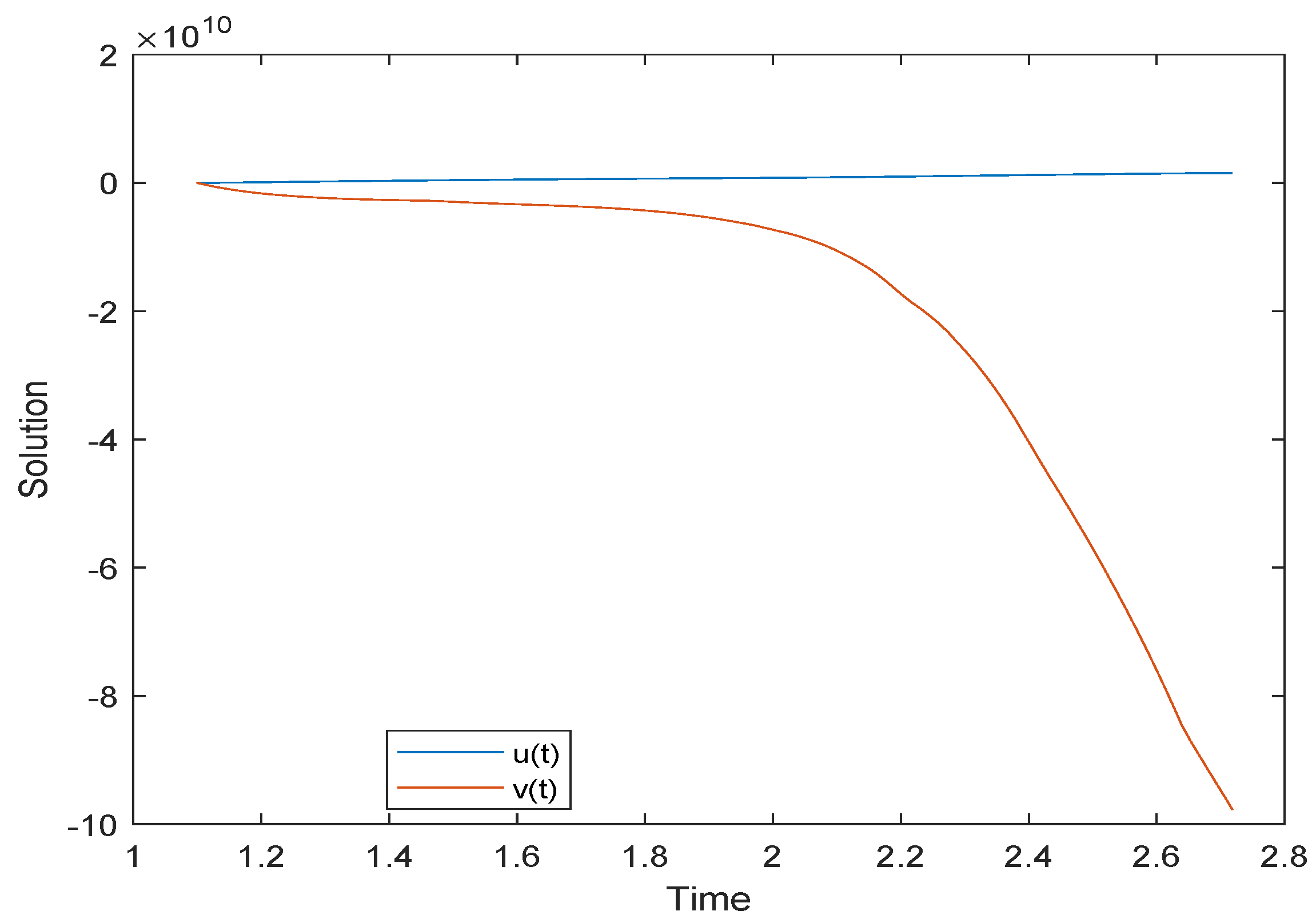
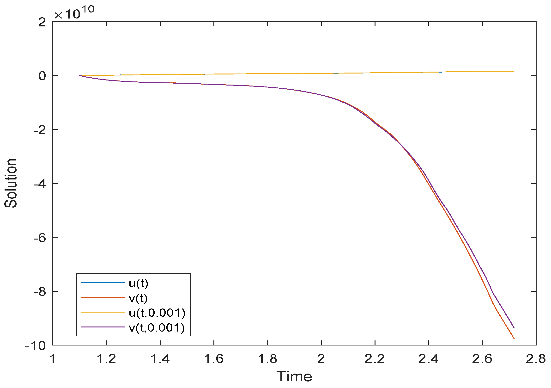
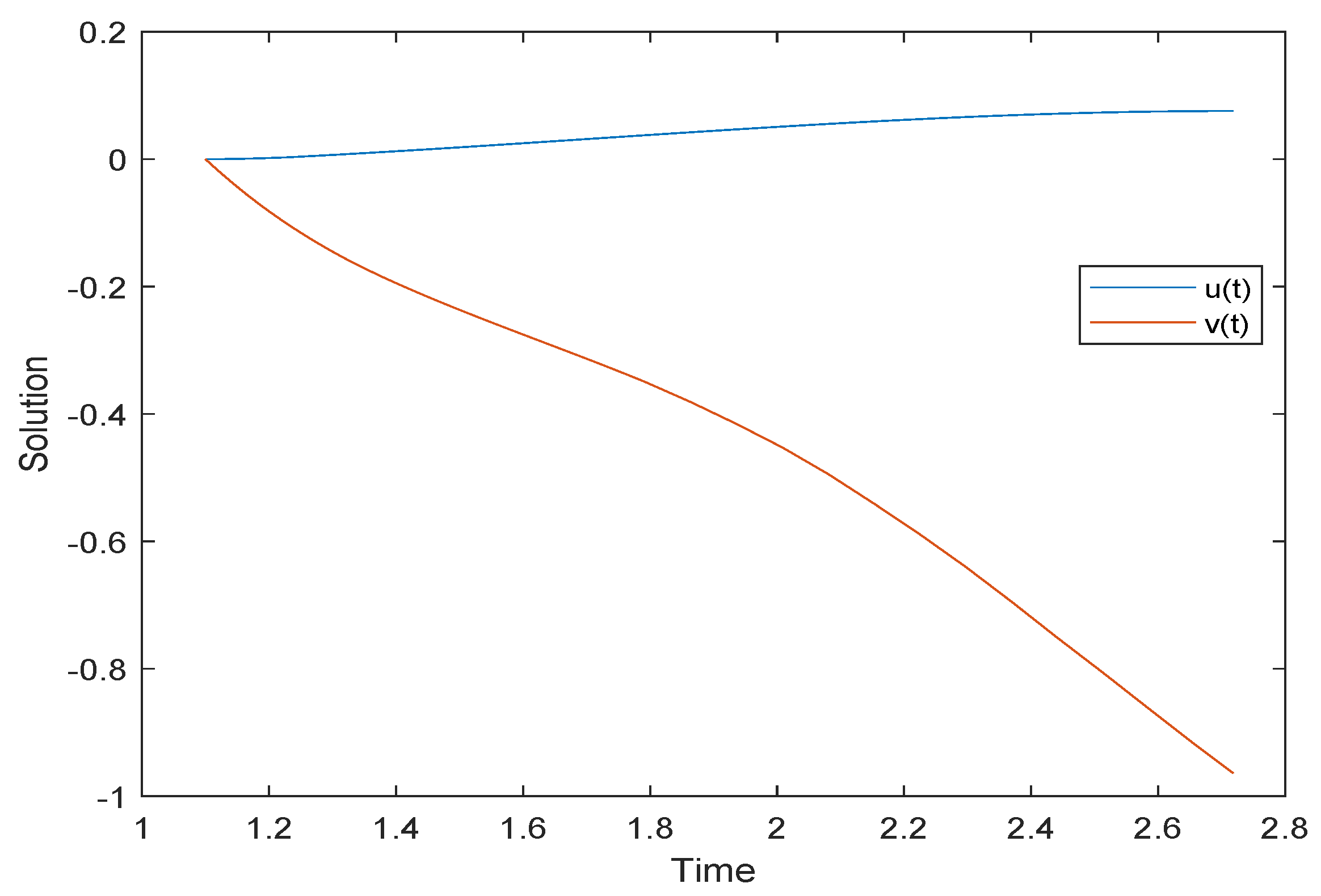
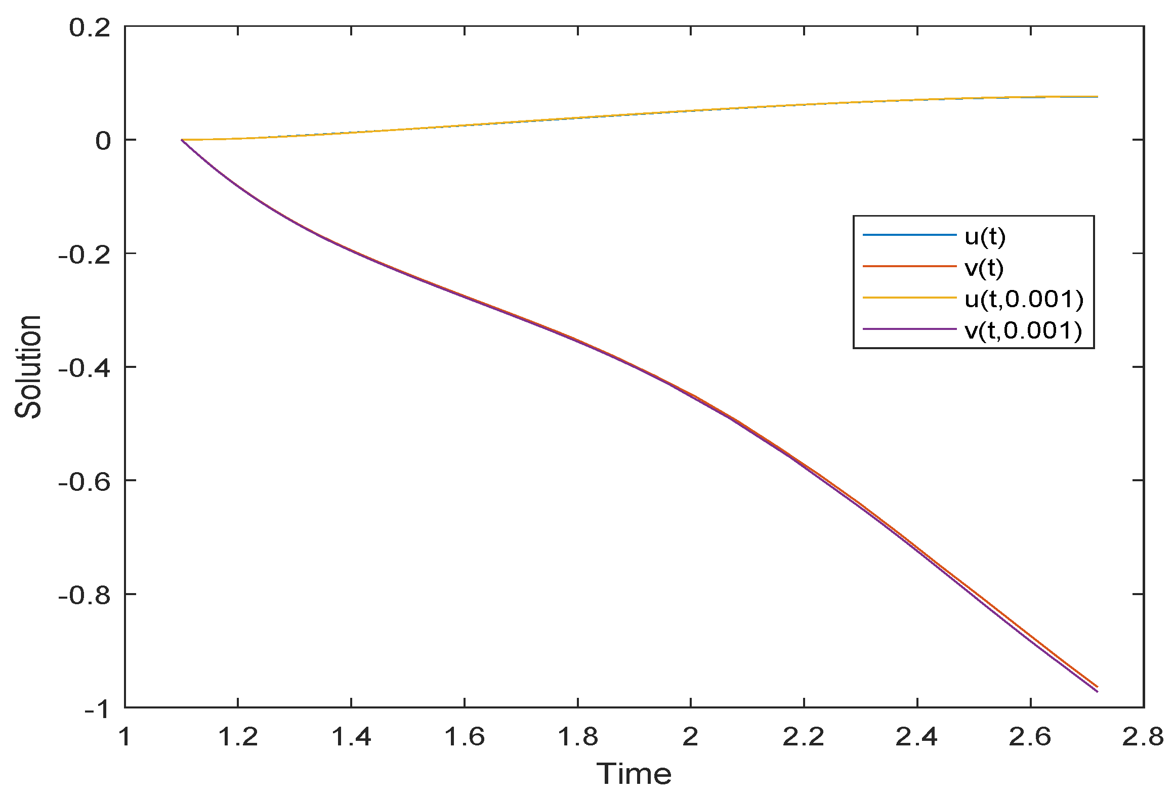
Based on the above algorithm, we employ the ODE113 toolbox in MATLAB R2019b on two examples to give their numerical solutions and simulations. Example 1 is shown as Table 1 and Table 2, Figure 1 and Figure 2. Example 2 is shown as Table 3 and Table 4, Figure 3 and Figure 4. Figure 2 and Table 1 and Table 2 show that Example 1 is GUH-stable. Figure 4 and Table 3 and Table 4 show that Example 2 is GUH-stable.
6. Summaries
It is well known that the -Laplacian differential equation arises from the turbulence problem in porous medium. In viscoelastic mechanics, some studies have shown that fractional order differential equation models are more accurate than integer order differential equation models. Therefore, the fractional -Laplacian differential model has greater advantages in the study of viscoelastic porous medium turbulence. In this article, we study BVP (1) of a nonlinear -Laplacian Hadamard fractional differential equation. Unlike many published papers, we have established the existence, uniqueness, stability, and sequence approximation of solutions for fractional order differential equations on a wide range of complete metric spaces rather than Banach spaces. We have obtained some concise and easily verifiable sufficient criteria. Examples 1 and 2 and simulations demonstrate that our main results are correct and available. Meanwhile, Figure 1 and Figure 2 also indicate that the solution of BVP (1) is sensitive and dependent on parameters and . Our results provide theoretical support for revealing the mechanical problems of viscoelastic porous medium turbulence. The mathematical theories and methods used in the article have certain generality in solving similar problems. In addition, based on our recent research findings [50,51,52,53], we plan to study some ecosystems involving fractional derivatives or reaction diffusion effects in the future.
Funding
The APC was funded by research start-up funds for high-level talents of Taizhou University.
Data Availability Statement
Not applicable.
Acknowledgments
The author would like to express his heartfelt gratitude to the reviewers for their constructive comments.
Conflicts of Interest
The author declares no conflict of interest.
References
- Leibenson, L. General problem of the movement of a compressible uid in a porous medium. Izv. Akad. Nauk Kirg. SSR Ser. Biol. Nauk 1983, 9, 7–10. [Google Scholar]
- Alsaedi, A.; Luca, R.; Ahmad, B. Existence of positive solutions for a system of singular fractional boundary value problems with -Laplacian operators. Mathematics 2020, 8, 1890. [Google Scholar] [CrossRef]
- Zhao, K.H. Solvability and GUH-stability of a nonlinear CF-fractional coupled Laplacian equations. AIMS Math. 2023, 8, 13351–13367. [Google Scholar]
- Rao, S.; Ahmadini, A. Multiple positive solutions for system of mixed Hadamard fractional boundary value problems with (p1,p2)-Laplacian operator. AIMS Math. 2023, 8, 14767–14791. [Google Scholar] [CrossRef]
- Alsaedi, A.; Alghanmi, M.; Ahmad, B.; Alharbi, B. Uniqueness of solutions for a ψ-Hilfer fractional integral boundary value problem with the -Laplacian operator. Demonstr. Math. 2023, 56, 20220195. [Google Scholar]
- Sun, B.; Zhang, S.; Jiang, W. Solvability of fractional functional boundary-value problems with -Laplacian operator on a half-line at resonance. J. Appl. Anal. Comput. 2023, 13, 11–33. [Google Scholar]
- Ahmadkhanlu, A. On the existence and multiplicity of positive solutions for a -Laplacian fractional boundary value problem with an integral boundary condition. Filomat 2023, 37, 235–250. [Google Scholar]
- Chabane, F.; Benbachir, M.; Hachama, M.; Samei, M.E. Existence of positive solutions for -Laplacian boundary value problems of fractional differential equations. Bound. Value Probl. 2022, 2022, 65. [Google Scholar] [CrossRef]
- Rezapour, S.; Abbas, M.; Etemad, S.; Minh Dien, N. On a multi-point -Laplacian fractional differential equation with generalized fractional derivatives. Math. Method. Appl. Sci. 2023, 46, 8390–8407. [Google Scholar] [CrossRef]
- Boutiara, A.; Abdo, M.; Almalahi, M.; Shah, K.; Abdalla, B.; Abdeljawad, T. Study of Sturm-Liouville boundary value problems with -Laplacian by using generalized form of fractional order derivative. AIMS Math. 2022, 7, 18360–18376. [Google Scholar] [CrossRef]
- Salem, A.; Almaghamsi, L.; Alzahrani, F. An infinite system of fractional order with -Laplacian operator in a tempered sequence space via measure of noncompactness technique. Fractal Fract. 2021, 5, 182. [Google Scholar] [CrossRef]
- Jong, K.; Choi, H.; Kim, M.; Kim, K.; Jo, S.; Ri, O. On the solvability and approximate solution of a one-dimensional singular problem for a -Laplacian fractional differential equation. Chaos Soliton Fract. 2021, 147, 110948. [Google Scholar]
- Li, S.; Zhang, Z.; Jiang, W. Multiple positive solutions for four-point boundary value problem of fractional delay differential equations with -Laplacian operator. Appl. Numer. Math. 2021, 165, 348–356. [Google Scholar] [CrossRef]
- Hadamard, J. Essai sur l’étude des fonctions données par leur développment de Taylor. J. Math. Pures Appl. 1892, 8, 101–186. [Google Scholar]
- Kilbas, A.A. Hadamard-type fractional calculus. J. Korean Math. Soc. 2001, 38, 1191–1204. [Google Scholar]
- Butzer, P.L.; Kilbas, A.A.; Trujillo, J.J. Compositions of Hadamard-type fractional integration operators and the semigroup property. J. Math. Anal. Appl. 2002, 269, 387–400. [Google Scholar] [CrossRef] [Green Version]
- Ahmad, B.; Ntouyas, S.K. On Hadamard fractional integro-differential boundary value problems. J. Appl. Math. Comput. 2015, 47, 119–131. [Google Scholar] [CrossRef]
- Aljoudi, S.; Ahmad, B.; Nieto, J.J.; Alsaedi, A. A coupled system of Hadamard type sequential fractional differential equations with coupled strip conditions. Chaos Soliton Fract. 2016, 91, 39–46. [Google Scholar]
- Benchohra, M.; Bouriah, S.; Graef, J.R. Boundary value problems for nonlinear implicit Caputo-Hadamard-type fractional differential equations with impulses. Mediterr. J. Math. 2017, 14, 206. [Google Scholar] [CrossRef]
- Huang, H.; Zhao, K.H.; Liu, X.D. On solvability of BVP for a coupled Hadamard fractional systems involving fractional derivative impulses. AIMS Math. 2022, 7, 19221–19236. [Google Scholar] [CrossRef]
- Zhao, K.H. Existence and UH-stability of integral boundary problem for a class of nonlinear higher-order Hadamard fractional Langevin equation via Mittag-Leffler functions. Filomat 2023, 37, 1053–1063. [Google Scholar] [CrossRef]
- Ulam, S. A Collection of Mathematical Problems-Interscience Tracts in Pure and Applied Mathmatics; Interscience: New York, NY, USA, 1906. [Google Scholar]
- Hyers, D. On the stability of the linear functional equation. Proc. Natl. Acad. Sci. USA 1941, 27, 2222–2240. [Google Scholar] [CrossRef] [Green Version]
- Zada, A.; Waheed, H.; Alzabut, J.; Wang, X. Existence and stability of impulsive coupled system of fractional integrodifferential equations. Demonstr. Math. 2019, 52, 296–335. [Google Scholar] [CrossRef]
- Yu, X. Existence and β-Ulam-Hyers stability for a class of fractional differential equations with non-instantaneous impulses. Adv. Differ. Equ. 2015, 2015, 104. [Google Scholar] [CrossRef] [Green Version]
- Zhao, K.H. Stability of a nonlinear fractional Langevin system with nonsingular exponential kernel and delay control. Discret. Dyn. Nat. Soc. 2022, 2022, 9169185. [Google Scholar] [CrossRef]
- Chen, C.; Li, M. Existence and Ulam type stability for impulsive fractional differential systems with pure delay. Fractal Fract. 2022, 6, 742. [Google Scholar] [CrossRef]
- Zhao, K.H. Existence, stability and simulation of a class of nonlinear fractional Langevin equations involving nonsingular Mittag-Leffler kernel. Fractal Fract. 2022, 6, 469. [Google Scholar] [CrossRef]
- Zhao, K.H. Stability of a nonlinear Langevin system of ML-type fractional derivative affected by time-varying delays and differential feedback control. Fractal Fract. 2022, 6, 725. [Google Scholar] [CrossRef]
- Mehmood, M.; Abbas, A.; Akgul, A.; Asjad, M.I.; Eldin, S.M.; Abd El-Rahman, M.; Baleanu, D. Existence and stability results for coupled system of fractional differential equations involving AB-caputo derivative. Fractals 2023, 31, 2340023. [Google Scholar] [CrossRef]
- Yaghoubi, H.; Zare, A.; Rasouli, M.; Alizadehsani, R. Novel frequency-based approach to analyze the stability of polynomial fractional differential equations. Axioms 2023, 12, 147. [Google Scholar] [CrossRef]
- Alqahtani, R.; Ntonga, J.; Ngondiep, E. Stability analysis and convergence rate of a two-step predictor-corrector approach for shallow water equations with source terms. AIMS Math. 2023, 8, 9265–9289. [Google Scholar]
- Salama, F.; Ali, N.; Hamid, N. Fast O(N) hybrid Laplace transform-finite difference method in solving 2D time fractional diffusion equation. J. Math. Comput. Sci. 2021, 23, 110–123. [Google Scholar] [CrossRef]
- Jassim, H.; Hussain, M. On approximate solutions for fractional system of differential equations with Caputo-Fabrizio fractional operator. J. Math. Comput. Sci. 2021, 23, 58–66. [Google Scholar] [CrossRef]
- Can, N.; Nikan, O.; Rasoulizadeh, M.; Jafari, H.; Gasimov, Y.S. Numerical computation of the time non-linear fractional generalized equal width model arising in shallow water channel. Therm. Sci. 2020, 24, 49–58. [Google Scholar] [CrossRef]
- Akram, T.; Abbas, M.; Ali, A. A numerical study on time fractional Fisher equation using an extended cubic B-spline approximation. J. Math. Comput. Sci. 2021, 22, 85–96. [Google Scholar] [CrossRef]
- Ahmad, I.; Ahmad, H.; Thounthong, P.; Chu, Y.M.; Cesarano, C. Solution of multi-term time-fractional PDE models arising in mathematical biology and physics by local meshless method. Symmetry 2020, 12, 1195. [Google Scholar] [CrossRef]
- Murtaza, S.; Ahmad, Z.; Ali, I.; Chu, Y.M.; Cesarano, C. Analysis and numerical simulation of fractal-fractional order non-linear couple stress nanofluid with cadmium telluride nanoparticles. J. King Saud Univ. Sci. 2023, 35, 102618. [Google Scholar] [CrossRef]
- Zhao, K.H. Generalized UH-stability of a nonlinear fractional coupling (p1,p2)-Laplacian system concerned with nonsingular Atangana-Baleanu fractional calculus. J. Inequal. Appl. 2023; accepted. [Google Scholar]
- Ahmad, Z.; Bonanomi, G.; di Serafino, D.; Giannino, F. Transmission dynamics and sensitivity analysis of pine wilt disease with asymptomatic carriers via fractal-fractional differential operator of Mittag-Leffler kernel. Appl. Numer. Math. 2023, 185, 446–465. [Google Scholar] [CrossRef]
- Ahmad, Z.; El-Kafrawy, S.; Alandijany, T.; Mirza, A.A.; El-Daly, M.M.; Faizo, A.A.; Bajrai, L.H.; Kamal, M.A.; Azhar, E.I. A global report on the dynamics of COVID-19 with quarantine and hospitalization: A fractional order model with non-local kernel. Comput. Biol. Chem. 2022, 98, 107645. [Google Scholar] [CrossRef]
- Ahmad, Z.; Ali, F.; Khan, N.; Khan, I. Dynamics of fractal-fractional model of a new chaotic system of integrated circuit with Mittag-Leffler kernel. Chaos Soliton. Fract. 2021, 153, 111602. [Google Scholar] [CrossRef]
- Wang, F.; Asjad, M.; Zahid, M.; Iqbal, A.; Ahmad, H.; Alsulami, M.D. Unsteady thermal transport flow of Casson nanofluids with generalized Mittag-Leffler kernel of Prabhakar’s type. J. Mater. Res. Technol. 2021, 14, 1292–1300. [Google Scholar] [CrossRef]
- Kilbas, A.A.; Srivastava, H.M.; Trujillo, J.J. Theory and Applications of Fractional Differential Equations; Elsevier: Amsterdam, The Netherlands, 2006. [Google Scholar]
- Rus, I.A. On a fixed point theorem of Maia. Stud. Univ. Babes-Bolyai Math. 1977, 22, 40–42. [Google Scholar]
- Wardowski, D. Fixed points of a new type of contractive mappings in complete metric spaces. Fixed Point Theory Appl. 2012, 2012, 94. [Google Scholar] [CrossRef] [Green Version]
- Agarwal, R.; O’Regan, D. Fixed point theory for generalized contractions on spaces with two metrics. J. Math. Anal. Appl. 2000, 248, 402–414. [Google Scholar] [CrossRef] [Green Version]
- Karapinar, E.; Fulga, A.; Agarwal, R. A survey: F-contractions with related fixed point results. J. Fixed Point Theory Appl. 2020, 22, 69. [Google Scholar] [CrossRef]
- Mehmood, N.; Khan, I.; Nawaz, M.; Ahmad, N. Existence results for ABC-fractional BVP via new fixed point results of F-Lipschitzian mappings. Demonstr. Math. 2022, 55, 452–469. [Google Scholar] [CrossRef]
- Zhao, K.H. Local exponential stability of several almost periodic positive solutions for a classical controlled GA-predation ecosystem possessed distributed delays. Appl. Math. Comput. 2023, 437, 127540. [Google Scholar] [CrossRef]
- Zhao, K.H. Existence and stability of a nonlinear distributed delayed periodic AG-ecosystem with competition on time scales. Axioms 2023, 12, 315. [Google Scholar] [CrossRef]
- Zhao, K.H. Global stability of a novel nonlinear diffusion online game addiction model with unsustainable control. AIMS Math. 2022, 7, 20752–20766. [Google Scholar] [CrossRef]
- Zhao, K.H. Attractor of a nonlinear hybrid reaction-diffusion model of neuroendocrine transdifferentiation of human prostate cancer cells with time-lags. AIMS Math. 2023, 8, 14426–14448. [Google Scholar] [CrossRef]
Figure 1.
Simulation of solutions to Example 1.

Figure 2.
Evolution of the GUH-stability of Example 1.

Figure 3.
Simulation of solutions to Example 2.

Figure 4.
Evolution of the GUH-stability of Example 2.


Table 1.
The numerical solution to Example 1 which needs to multiply by .
| t | 1.2 | 1.4 | 1.6 | 1.8 | 2.0 | 2.2 | 2.4 | 2.6 | 2.7183 | |
|---|---|---|---|---|---|---|---|---|---|---|
| u | ||||||||||
| 0.0079 | 0.0314 | 0.0497 | 0.0645 | 0.0786 | 0.0963 | 0.1210 | 0.1448 | 0.1501 | ||
| 0.0080 | 0.0318 | 0.0501 | 0.0650 | 0.0790 | 0.0971 | 0.1218 | 0.1447 | 0.1498 | ||
Table 2.
The numerical solution to Example 1 which needs to multiply by .
| t | 1.2 | 1.4 | 1.6 | 1.8 | 2.0 | 2.2 | 2.4 | 2.6 | 2.7183 | |
|---|---|---|---|---|---|---|---|---|---|---|
| u | ||||||||||
| 0.1653 | 0.2690 | 0.3344 | 0.4302 | 0.7319 | 1.7307 | 4.0310 | 7.5843 | 9.7746 | ||
| 0.1671 | 0.2720 | 0.3355 | 0.4327 | 0.7319 | 1.7749 | 3.9019 | 7.2621 | 9.3765 | ||
Table 3.
The numerical solution to Example 2.
| t | 1.2 | 1.4 | 1.6 | 1.8 | 2.0 | 2.2 | 2.4 | 2.6 | 2.7183 | |
|---|---|---|---|---|---|---|---|---|---|---|
| u | ||||||||||
| 0.0018 | 0.0121 | 0.0252 | 0.0384 | 0.0507 | 0.0614 | 0.0699 | 0.0749 | 0.0757 | ||
| 0.0019 | 0.0122 | 0.0254 | 0.0387 | 0.0511 | 0.0619 | 0.0704 | 0.0754 | 0.0763 | ||
Table 4.
The numerical solution to Example 2 which needs to multiply by .
| t | 1.2 | 1.4 | 1.6 | 1.8 | 2.0 | 2.2 | 2.4 | 2.6 | 2.7183 | |
|---|---|---|---|---|---|---|---|---|---|---|
| u | ||||||||||
| 0.0818 | 0.1947 | 0.2757 | 0.3530 | 0.4481 | 0.5721 | 0.7189 | 0.8741 | 0.9639 | ||
| 0.0824 | 0.1960 | 0.2779 | 0.3556 | 0.4516 | 0.5767 | 0.7244 | 0.8828 | 0.9723 | ||
Disclaimer/Publisher’s Note: The statements, opinions and data contained in all publications are solely those of the individual author(s) and contributor(s) and not of MDPI and/or the editor(s). MDPI and/or the editor(s) disclaim responsibility for any injury to people or property resulting from any ideas, methods, instructions or products referred to in the content. |
© 2023 by the author. Licensee MDPI, Basel, Switzerland. This article is an open access article distributed under the terms and conditions of the Creative Commons Attribution (CC BY) license (https://creativecommons.org/licenses/by/4.0/).
Share and Cite
MDPI and ACS Style
Zhao, K.
Solvability, Approximation and Stability of Periodic Boundary Value Problem for a Nonlinear Hadamard Fractional Differential Equation with
AMA Style
Zhao K.
Solvability, Approximation and Stability of Periodic Boundary Value Problem for a Nonlinear Hadamard Fractional Differential Equation with
Zhao, Kaihong.
2023. "Solvability, Approximation and Stability of Periodic Boundary Value Problem for a Nonlinear Hadamard Fractional Differential Equation with
Note that from the first issue of 2016, this journal uses article numbers instead of page numbers. See further details here.