
Finite-Time Passivity and Synchronization for a Class of Fuzzy Inertial Complex-Valued Neural Networks with Time-Varying Delays

School of Information Engineering, Wuhan Business University, Wuhan 430056, China
Axioms 2024, 13(1), 39; https://0-doi-org.brum.beds.ac.uk/10.3390/axioms13010039
Submission received: 12 December 2023
/
Revised: 29 December 2023
/
Accepted: 3 January 2024
/
Published: 7 January 2024
(This article belongs to the Special Issue Control Theory and Control Systems: Algorithms and Methods)
Abstract
:This article investigates finite-time passivity for fuzzy inertial complex-valued neural networks (FICVNNs) with time-varying delays. First, by using the existing passivity theory, several related definitions of finite-time passivity are illustrated. Consequently, by adopting a reduced-order method and dividing complex-valued parameters into real and imaginary parts, the proposed FICVNNs are turned into first-order real-valued neural network systems. Moreover, appropriate controllers and the Lyapunov functional method are established to obtain the finite-time passivity of FICVNNs with time delays. Furthermore, some essential conditions are established to ensure finite-time synchronization for finite-time passive FICVNNs. In the end, corresponding simulations certify the feasibility of the proposed theoretical outcomes.
Keywords:
fuzzy inertial complex-valued neural networks; finite-time passivity; finite-time synchronizationMSC:
34K20; 93D031. Introduction
As is known to all, the neural networks as a hot direction of non-linear systems have aroused the interest of experts and scholars due to their fruitful applications, including artificial intelligence, pattern recognition, associative memories, etc. Many worthy related results have been explored in recent years [1,2,3].
However, plenty of existing articles mainly gather in the first derivative of the states instead of the inertial term, which is the second derivative of voltage concerning time. Hence, based on the Hopfield networks, inertial neural networks (INNs) were put forward by Babcock. As mentioned in this document [4], the dynamic behaviors of second-derivative neural networks could be more sophisticated. During these years, some corresponding results on inertial neural networks (INNs) have been reported [5,6,7,8,9]. Tu et al. [10] discussed the issue of global dissipativity for INNs with memristor-based neutral type using the Filippov theory and LMI approach. In [11], Shanmugasundaram et al. introduced the event-triggered impulsive control mechanism to guarantee synchronization for INNs. Zhang and Cao [12] considered the INNs using inequality techniques to obtain finite-time synchronization. As to the asymptotical stabilization problem, Han et al. [13] used a direct method to analyze the Cohen–Grossberg INNs and constructed two adaptive controllers to make the proposed model realize asymptotical and adaptive stabilization. In [14], the authors were concerned with the issue of global exponential convergence for impulsive INNs and presented an exponential convergence ball with a specified convergence rate.
Admittedly, time delays can easily provoke certain undesirable and unexpected dynamical behaviors and diverse types of time delays, including proportional delay [15,16], time-varying delay [17,18], and mixed delays [19,20]. Moreover, the exchange of neural network systems depends on the current state and the paste state or the variations of the paste state. From the theoretical and particle view, time delays are deeply researched for INN instability [21,22], passivity [23,24], synchronization [11,12,16,25,26], dissipativity [27,28], and so forth.
In many circumstances, the complex-valued neural networks (CVNNs), which activate functions, connection parameters, neuron states, and so forth, are both complex-valued [29,30,31,32,33,34,35]. Consequently, it becomes an expansion of real-valued networks. The original intention of investigating CVNNs is to research novel dynamic behaviors and to conquer some puzzles that real-valued networks can not describe [36]. Furthermore, the inertial complex-valued neural networks (ICVNNs) have become a hot theme that has attracted some researchers’ attention, especially stability and synchronization [37]. Tang and Jian [38] carry out the exponential convergence for impulsive ICVNNs by developing novel delay-dependent conditions. In [39], the authors emphasized the non-reduced order method to deal with ICVNNs holistically to discuss the question of exponential and adaptive synchronization by constructing a complex-valued feedback control input. Long and Zhang et al. observed the finite-time stabilization and fixed-time synchronization of ICVNNs by utilizing Lyapunov theory and inequality techniques applied theoretical results into practical [40,41].
As a typical and essential problem, fuzzy logic has extensively emerged because it can approximate non-linear functions with arbitrary accuracy, which can be viewed as a potential method by which to emulate human thinking and sensation [42]. Hence, Combining fuzzy logic into a neural network system has been received high concern [43]. On the other hand, as [9] reveals, stabilization and synchronization of many practical engineering systems are required in a finite-time, which lead to the previous results of asymptotic stabilization and synchronization control inoperative. Therefore, it is vital to shorten the convergence time to achieve finite-time synchronization of complex-valued neural networks. In [44], the authors dealt with the question on fixed-time stabilization of fuzzy inertial neural networks (FINNs). The issues of synchronization for FINNs have been addressed in [16,19]. Xiao et al. study the passive and passification for FINNs on time scales inspired by the LMI method and analytical approaches [45]. Furthermore, the authors of [46] developed fuzzy rules into CVNNs and established a class of fuzzy inertial complex-valued neural networks (FICVNNs) to solve the adaptive synchronization problem.
Passivity is a powerful tool for investigating the internal stability of non-linear systems. It is originally from circuit analysis methods that have received much attention from the engineering fields and dynamical neural networks. And some related passivity problems for neural networks have been published [23,24,33,35,45,47,48,49]. The authors in [24,35,45,48,49] studied the passivity problem for different types of neural networks. Huang et al. [33] further learned the passivity issues for CVNNs with coupled weights. Motivated by the above analysis, based on the existing passivity theory, when it comes to discussing FICVNNs with time-varying delays, some related puzzles naturally arise; for example, how to ensure the proposed FICVNNs realize finite-time passivity (FTP), finite-time input strict passivity (FTISP), as well as finite-time output strictly passivity (FTOSP)? If it can be done, what kind of Lyapunov functional and control inputs are supposed to realize the corresponding passivity goal? Is there any relation between the FTP and FTS? As far as we are concerned, few documents carried out the FTP and FTS of FICVNNs, making this work remarkable and valuable. The main contributions of this article are as follows.
First, by resorting to existing passivity definitions, three concepts of finite-time passivity are illustrated. Moreover, the neural model built in this paper is concerned with inertial terms, complex-valued parameters, fuzzy logic, and time delays, which will increase the difficulty and complexity of solving the neural systems internally stable.
Second, compared with [24,35,45,48,49], we use effective control inputs and the appropriate Lyapunov function to gain some finite-time passivity criteria for delayed FICVNNs.
Third, based on the finite-time passivity, we further discuss the finite-time synchronization issue and apply the simulations about pseudorandom number generators to support the feasibility of the obtained results.
2. Preliminaries
Model, Assumption, Definitions, and Lemmas
Here, and , respectively, denote the n-dimensional complex vector space and the real vector space with n-dimensional. For any , i is the imaginary unit and meets , implies the real part of v, and is the imaginary part. , For any , , , .
Now, a class of FICVNNs with time-varying delays is given:
where , , is the state of kth neural at time t, and are positive constants, and denote the feedback connection weights of system (1). presents the feedback function, is the time-varying delay, and and . and imply the fuzzy feedback MIN and MAX template. represent fuzzy AND, OR. The initial conditions of FIVCNNs (1) are
where , , , and . With regard to active function , we introduce the following assumption.
Assumption 1.
As to activation function , , it can be divided by the real part and the imaginary part, such as . And, for any , the real part , as well as the imaginary part of the activation function , can be characterized by
where are non-negative constants.
For certain positive scalar , we make the variable transformation:
then, we have
Considering system (4) as the driver system, let , , , , , , , , , , , , , .
Therefore, the matrix form of system (4) can be described by
then, the matrix form of the response system is as follows:
where are control schemes; that is, and . represents external input which . Based on Assumption 1, system (7) can be transformed as follows:
and response system (8) can be represented by
Considering , , , . , , , . Through (9) and (10), we obtain the following error system
Next, we give some necessary definitions as follows.
Definition 1
([47]). Suppose that the output in system and input obtain finite-time passivity (FTP) for any and , if
where stands for a non-negative function.
Definition 2
([47]). Suppose that the output in system and input obtain finite-time input strict passivity (FTISP) for any and , if
where stands for a non-negative function.
Definition 3
([47]). Suppose that the output in system and input obtain finite-time input strict passivity (FTOSP) for any and , if
where stands for a non-negative function.
Lemma 1
([50]). It is assumed that with a continuous and non-negative function which satisfies
where and , it can determined that,
and
thus, we obtain
Remark 1.
Many compelling results about passivity have been reported [48,49]. However, these references only pat attention to the input or output passivity problems, making the system only realize the infinite-time input or output passivity. Moreover, as [24,35,47] reveals, passivity can be an effective tool for discussing infinite-time synchronization for neural systems. But, from a practical perspective, the setting time of synchronization should be finite is more reasonable. Hence, the research in the paper is more general and extends the existing passivity theory.
Lemma 2
Lemma 3
Remark 2.
Passivity analysis for real-valued neural networks (RVNNs) is widely observed [23,24,35,45,47,48,49], in which activation function, connection weight, input, and output are real-valued. Compared with RVNNs, CVNNs can viewed as a more general case because of more complex dynamic characteristics. Such symmetry detection and XOR issues are expected to be solved by CVNNs easily but cannot be settled by RVNNs [36]. In addition, compared with [23,24,33,35,49], inertial terms and fuzzy logic cases are supposed to cause complex essential impacts on dynamics behaviors for network systems. To our knowledge, few corresponding outcomes focus on the model with these elements. Therefore, it is significant to devote our effort to providing a guide for this analysis.
Remark 3.
Suppose that an energy function stands for the energy stored in this system, and the energy supply bounded over finite-time intervals, then we call the system passive. As to storage function and supply rate , compared with [23,47], we develop FTP, FTISP, and FTOSP from real-valued into complex-valued, and different supply rate reveals that the dissipative of inside the system is not more than the external source .
3. Main Results
3.1. Finite-Time Passivity
Let the controller be , , and , , , are constructed as follows:
in which and denote the positive definite gain matrices; and ; when ,
, are the same defined as , , respectively. and are the same, defined as and , respectively.
What is more,
when .
We define the output vector of system (11):
where . For convenience, we let
Theorem 1.
The network system (11) obtain FTP under control inputs (19) and (20) if there exist
satisfying such conditions as
where , , , , , , . , , and E is the identity matrix.
Proof.
where
Case 1. When , we build the Lyapunov function as follows:
where
Then, when , we arrange the derivative of as
under Assumption 1, from (28), then
In addition, according to Lemma 3, one has
Moreover,
Likewise, from Lemma 2, one has
Similarly,
What is more,
Because of (30)–(35), it is arranged by
and
Furthermore,
Consequently, it concludes that
where , , and .
Case 2. When , the Lyapunov function is
Arranging the derivative of , one has
Moreover,
where and .
Based on the above analysis, according to Definition 1, system (11) can realize FTP under controller (19). At the instant time t when , we also can infer that system (11) achieves FTP by controller (20). Therefore, system (9) can reach FTP under control schemes (19) and (20). □
Theorem 2.
Under the condition of Theorem 1, the network (11) can realize FTISP through controllers (19) and (20) if there are
where , , , , , , , , have the same meanings as in Theorem 1, and .
Proof.
Building the same Lyapunov function as (25), combining with (46) and (47), we can carry out
Then, one attains
where , , , . Consequently, system (11) can achieve FTISP under controller (19). When , the proving procedure has a resemblance to Theorem 1 and is omitted here. So, based on Definition 2, the system (11) can obtain FTISP through controller (19) and (20). □
Theorem 3.
Under the condition of Theorem 1, the network (11) can realize FTOSP through controllers (19) and (20) if there are
where , , , , , , . , .
Proof.
where , , , . Then, one derives
Considering the same Lyapunov function as (25), combined with (46) and (47), it follows that
Consequently, the system (11) can achieve FTOSP under controller (19). When , the proving procedure has a resemblance to Theorem 1 which is omitted here. So, based on Definition 2, the system (11) can obtain FTISP through controllers (19) and (20). □
3.2. Finite-Time Synchronization
Theorem 4.
Suppose that : is a differentiable continuous function which has
where stands for a strictly monotonically continuous increasing function, for , is positive with If network system (11) obtains FTP (FTISP, FTOSP) through control inputs (19) and (20), the networks (9) and (10) reach FTS based on controllers (19) and (20).
Proof.
If system (11) realizes FTP under controllers (19) and (20), there exist and , such that
Considering , we have
From Lemma 1, we obtain for , .
Because of
one attains
where . Then, we can derive . Namely, the system (9) and (10) arrive at FTS under controller (19) and (20). Similarly, when system (11) obtains FTISP and FTOSP, we can deduce that system (9) and (10) reach FTS under control inputs (19) and (20). □
Corollary 1.
If there exist
satisfying such conditions as
where , , , , , , , , and are same as in Theorem 1, then FICVNN (1) is a finite-time synchronization based on controllers (19) and (20).
Remark 4.
Commonly, it is not easy to deal with passivity and synchronization in real-valued neural network systems, let alone solve the problem of FTP and FTS with complex-valued parameters. Furthermore, owing to inertial terms and fuzzy logic, traditional ways can not directly deal with the FTP and FTS of FICVNNs. To conquer these points, in this paper, some suitable control inputs and novel Lyapunov functionals are divided into the real part and the imaginary part to ensure that FICVNNs are addressed to obtain passivity and synchronization in a finite time interval.
3.3. Example
Example 1.
Think about the delayed FICVNNs as follows:
Through Formulae (3) and (4), the matrix form of system (65) is demonstrated by
where , , , , , , , , , , , , , , , , , , , , , , , , , , . The initial conditions of the system (65) are selected as , , , . Then, Figure 1, Figure 2 and Figure 3 show the trajectories of states without control. Moreover, consider system (66) as a drive system; the response system is
where , m(t) are controllers given in formula (19), I(t) is external input, , . We select , , and as follows:
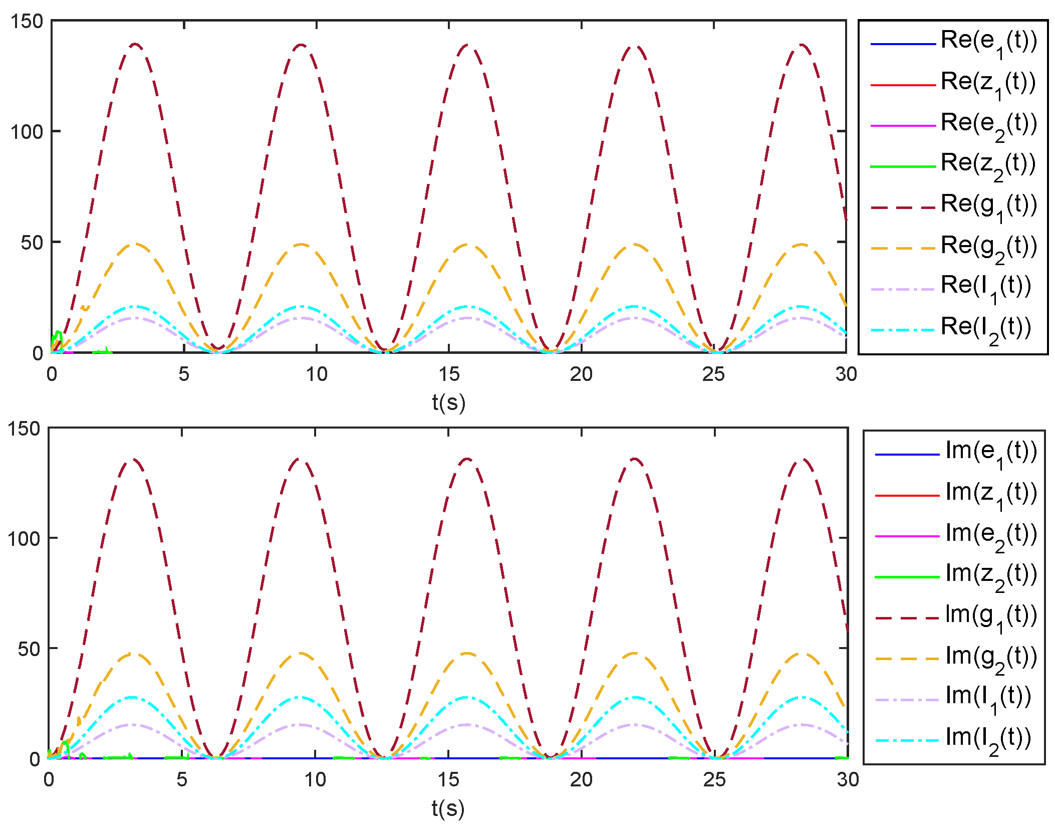
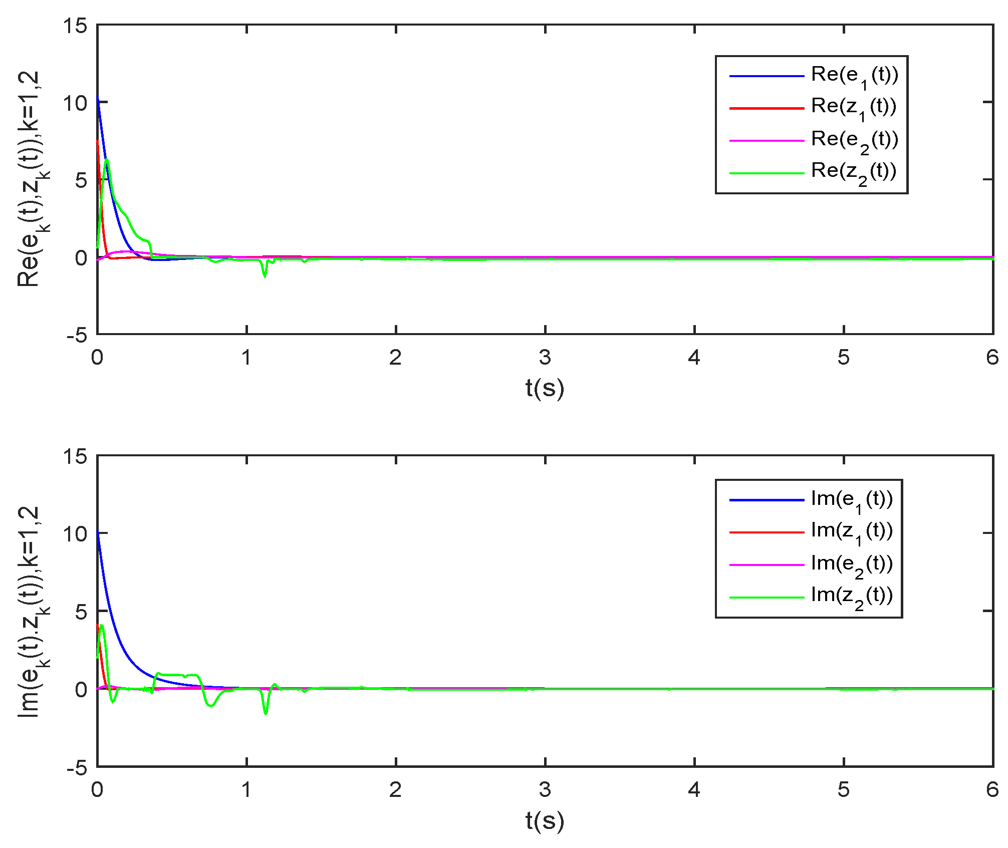
The rest of parameters are the same as in system (66). In addition, the parameters in (19) are selected as , , , , and . Take and , which satisfy the condition of Theorem 1. Through Theorem 1, the network in (65) obtains FTP under controller (19). Take , , and , which satisfy the condition of Theorem 2; (65) achieves FTISP under controller (19). Take , , and , and one can satisfy the condition of Theorem 3. In terms of Theorem 3, system (65) can realize the FTOSP under controller (19). Above all, the simulation of dynamical changes for state error , , input , and output are given in Figure 4.
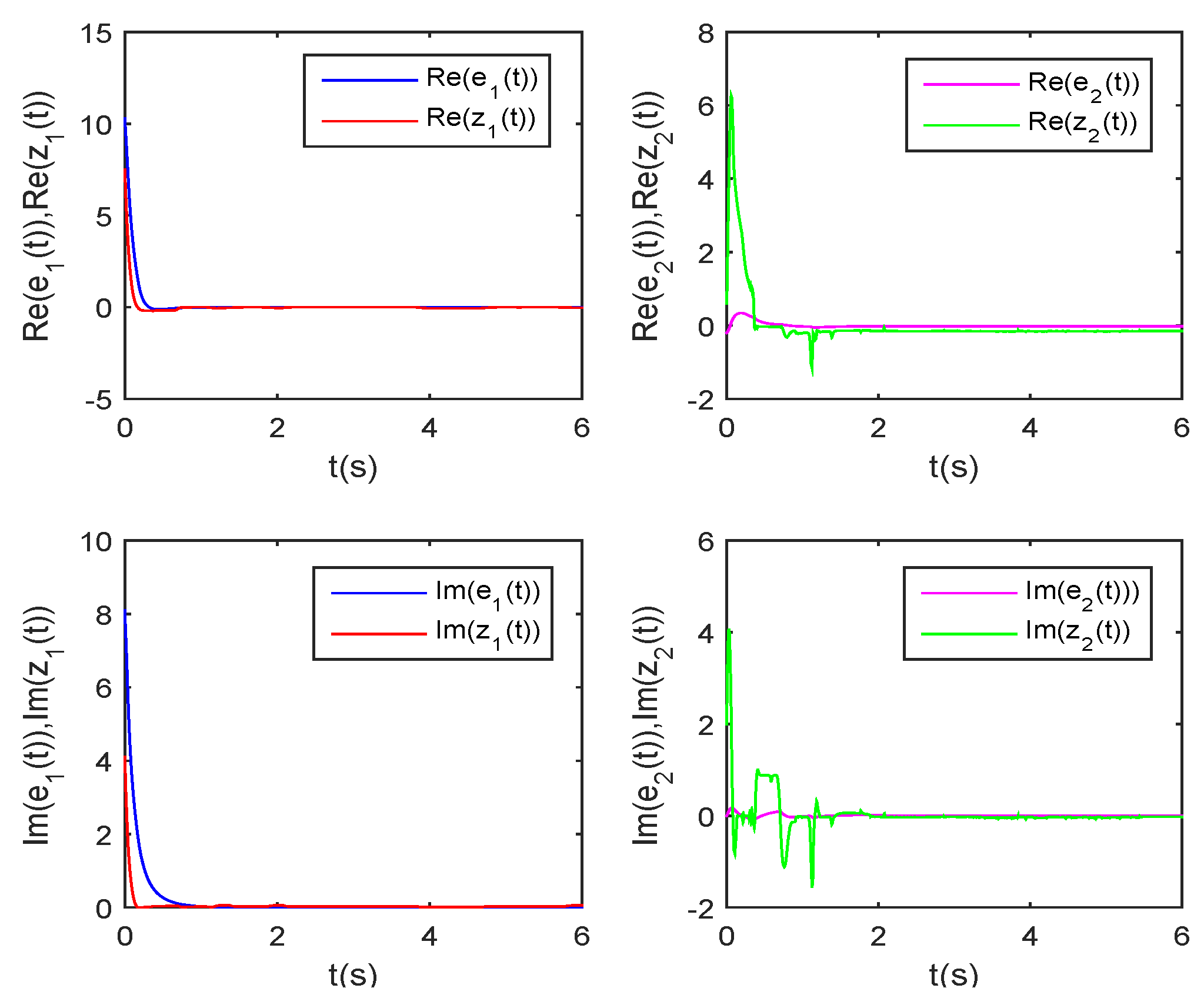
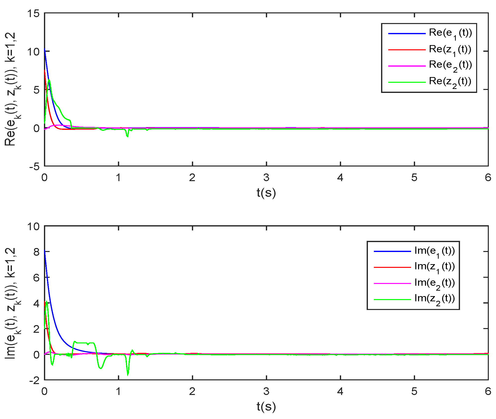
Let , , , , . Figure 5 denotes the trajectories of state error , and , with controller (19) when (65) is finite-time passive. The state trajectories of state error , , and , , , respectively, are illustrated in Figure 6.
According to Corollary 1, the network (65) with the above parameters can realize FTS under controller (19), and the setting time is computed as . As Figure 7 reveals, when time increases to 5.904, the corresponding simulation curves of the state error , and , tend to 0. This demonstrates that network (65) can achieve finite-time synchronization.
Example 2.
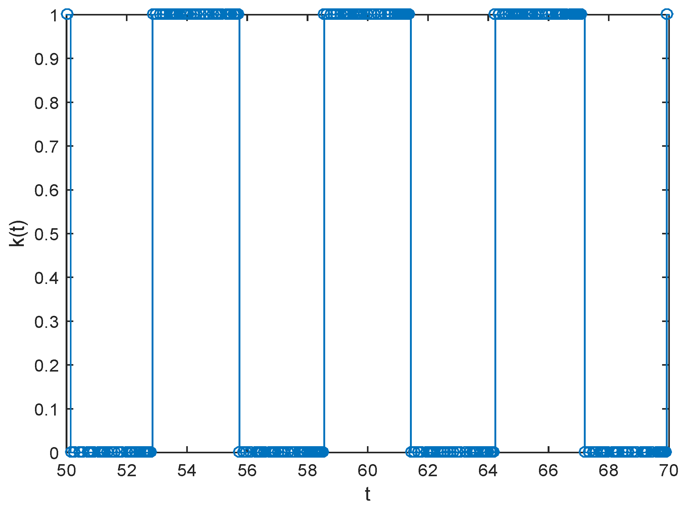
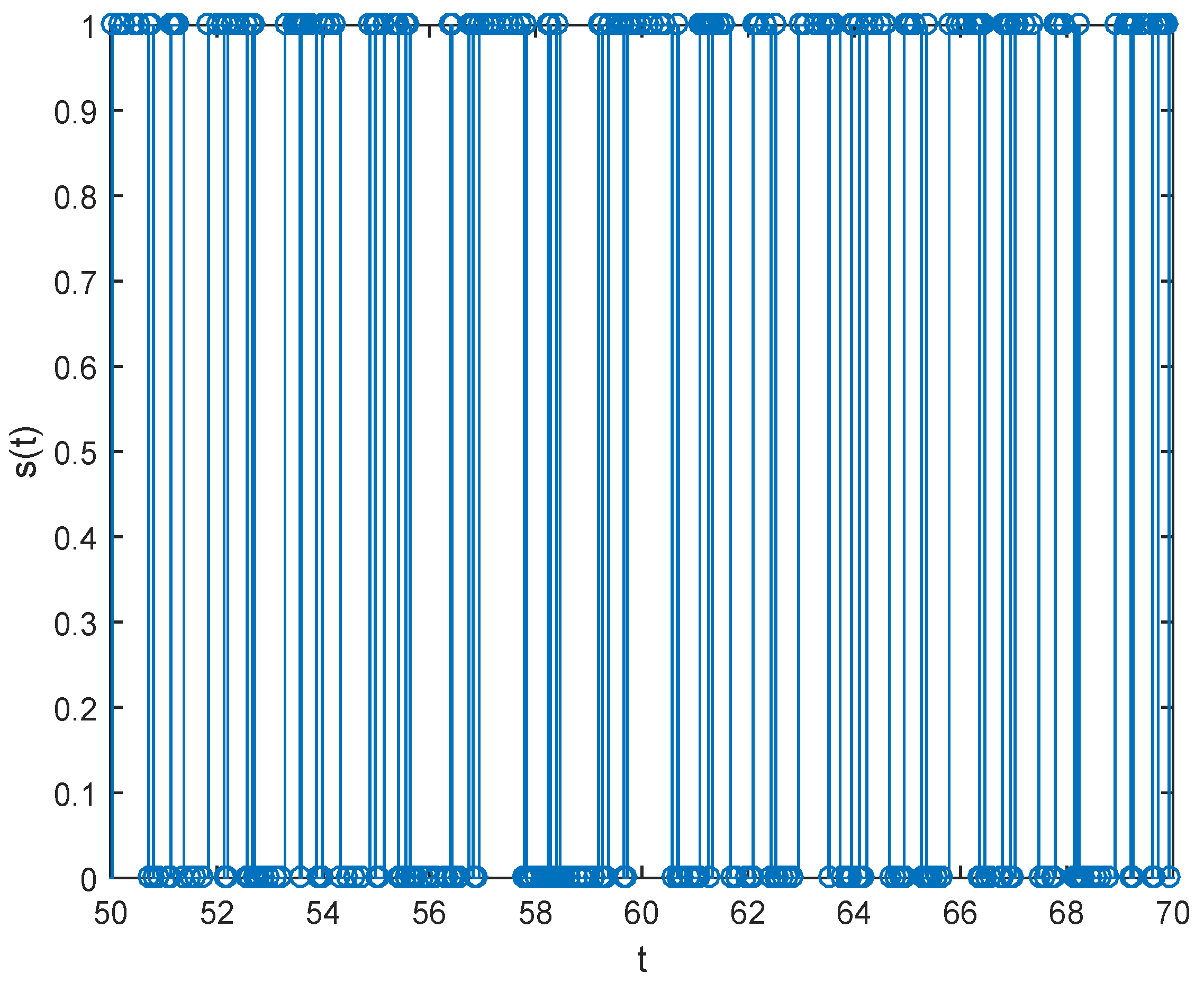
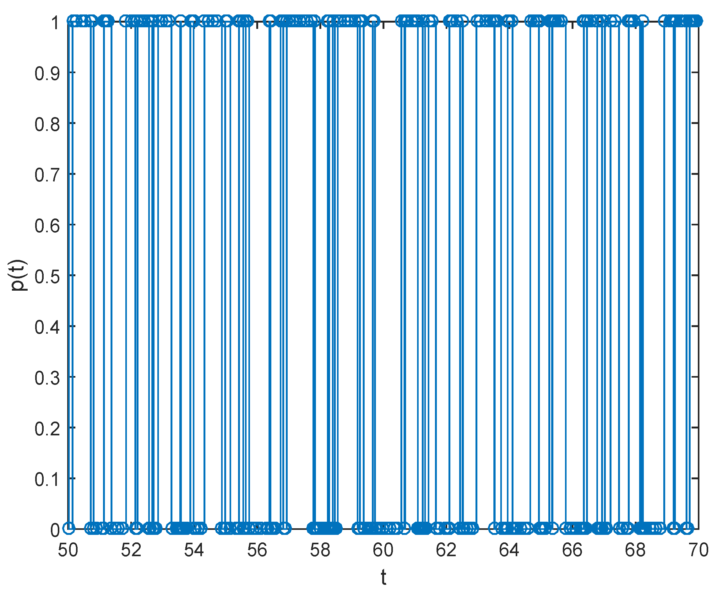
The application example of FICVNNs (65) relates to the pseudorandom number generator (PRNG) [43]. Let a sequence of pseudorandom number , stand for the operating time interval; then, one has
where
4. Conclusions
This article investigated the finite-time passivity and finite-time synchronization of the proposed FICVNNs with time delays. By transforming the second-order complex-valued model into first-order real-valued differential systems, the Lyapunov functional method and some novel controllers are explored to guarantee the FTP, FTISP, and FTOSP of FICVNNs. Furthermore, based on finite-time passive FICVNNs, finite-time synchronization has been investigated. Finally, some numerical simulations are provided to confirm the theory results.
Some existing works have discussed the passive properties of neural network systems that can maintain the system’s internal stability. For example, the infinite-time passivity or infinite-time synchronization of neural networks is generally considered by resorting to passivity theory [24,35,49]. Compared with the above literature, the neural model built in this paper, with inertial terms, complex-valued parameters, fuzzy logic, and time delays, enriches and expands previous results. It is supposed to create a foundation for observing the creative controllers for fixed-time synchronization or predefined-time synchronization in neural networks [9,51]. Compared with [33], we can also develop the related results to fit inertial neural networks, the parameters of the systems state-dependently switching. This is an essential and valuable direction in investigating various kinds of neural networks with more control methods in the future.
Funding
This research received no external funding.
Data Availability Statement
Data are contained within the article.
Conflicts of Interest
The author declares that they have no known competing financial interest or personal circumstances that could have appeared to influence the work reported in this manuscript.
References
- Xiao, J.Y.; Li, Y.T.; Wen, S.P. Mittag-Leffler synchronization and stability analysis for neural networks in the fractional-order multi-dimension field. Knowl.-Based Syst. 2021, 231, 107404. [Google Scholar] [CrossRef]
- Soltani, A.; Abadi, S. A novel control system for synchronizing chaotic systems in the presence of communication channel time delay; case study of Genesio-Tesi and Coullet systems. Nonlinear Anal. Hybrid Syst. 2023, 50, 101408. [Google Scholar]
- Huang, X.Q.; Lin, W.; Yang, B. Global finite-time stabilization of a class of uncertain nonlinear systems. Automatica 2005, 41, 881–888. [Google Scholar] [CrossRef]
- Wheeler, D.W.; Schieve, W.C. Stability and chaos in an inertial two-neuron system. Physica D 1997, 105, 267–284. [Google Scholar] [CrossRef]
- Jian, J.G.; Duan, L. Finte-time synchronization for fuzzy neutral-type inertial neural networks with time-varyiing coefficients and proportional delyas. Fuzzy Set Syst. 2020, 381, 51–67. [Google Scholar] [CrossRef]
- Rakkiyappan, R.; Premalatha, S.; Chandrasekar, A.; Cao, J.D. Stability and synchronization analysis of inertial memrisitve nerual networks with time delays. Cogn. Neurodyn. 2016, 10, 437–451. [Google Scholar] [CrossRef]
- Prakash, M.; Balasubramaniam, P.; Lakshmanan, S. Synchroinization of Markovian jumping inertial neural networks and its applications in image encryption. Neural Netw. 2016, 83, 86–93. [Google Scholar] [CrossRef]
- Zhang, W.; Huang, T.; He, X.; Li, C. Global exponential stability of inertial memristor-based neural networks with time-varying delayed and impulses. Neural Netw. 2017, 95, 102–109. [Google Scholar] [CrossRef]
- Han, J.; Chen, G.C.; Hu, J.H. New results on anti-synchronization in predefined-time for a class of fuzzy inertial neural networks with mixed time delays. Neurocomputing 2022, 495, 26–36. [Google Scholar] [CrossRef]
- Tu, Z.W.; Cao, J.; Alsaedi, A.; Alsaadi, F. Global dissipativity of memristor-based neutral type inertial neural networks. Neural Netw. 2017, 88, 125–133. [Google Scholar] [CrossRef]
- Shanmugasundaram, S.; Udhayakumar, K.; Gunasekaran, D.; Rakkiyappan, R. Event-triggered impulsive control design for synchronization of inertial neural networks with time delyas. Neurocomputing 2022, 483, 322–332. [Google Scholar] [CrossRef]
- Zhang, Z.Q.; Cao, J.D. Novel finite-time synchronization criteria for inertial neural networks with time delays via integral inequality method. IEEE Trans. Neural Netw. Learn. Syst. 2019, 30, 1476–1485. [Google Scholar] [CrossRef] [PubMed]
- Han, S.Y.; Hu, C.; Yu, J.; Jiang, H.J.; Wen, S.P. Stabilization of inertial Cohen-Grossberg neural netwroks with generalized delays: A direct analysis approah. Chaos Solitons Fractals 2021, 142, 110432. [Google Scholar] [CrossRef]
- Wan, P.; Jian, J. Global convergence analysis of impulsive inertial neural networks with time-varying delays. Neurocomputing 2017, 245, 68–76. [Google Scholar] [CrossRef]
- Alimi, A.M.; Aouiti, C.; Assali, E.A. Finte-time and fixed-time synchronization of a class of inertial nerual networks with multi-proportional delays and its application to secure communication. Neurocomputing 2019, 332, 29–43. [Google Scholar] [CrossRef]
- Duan, L.Y.; Li, J.M. Fixed-time synchronization of fuzzy neutral-type BAM meeristive inertial neural networks with proportional delays. Inf. Sci. 2021, 576, 522–541. [Google Scholar] [CrossRef]
- Kong, F.C.; Ren, Y.; Sakthivel, R. Delay-dependent crteria for periodicity and exponential stability of inertial neural networks with time-varying delays. Neurocomputing 2021, 419, 261–272. [Google Scholar] [CrossRef]
- Zheng, C.C.; Yu, J.; Jiang, H.J. Fixed-time synchronization of discontinuous competitive neural networks with time-varying delays. Neural Netw. 2022, 153, 192–203. [Google Scholar] [CrossRef]
- Cao, Y.T.; Wang, S.Q.; Guo, Z.Y.; Huang, T.W.; Wen, S.P. Stabilization of memristive neural networks with mixed time-varying delays via continuous/periodic event-based control. J. Frankl. Inst. 2020, 357, 7122–7138. [Google Scholar] [CrossRef]
- Kumar, R.; Das, S. Exponential stability of inertial BAM neural network with time-varying impulses and mixed time-varying delays via matrix measure approach. Commun. Nonlinear Sci. Number. Simul. 2020, 81, 105016. [Google Scholar] [CrossRef]
- Zhang, G.D.; Zeng, Z.G. Stabilization of second-order memristive neural networks with mixed time delays via non-reduced order. IEEE Trans. Neural Netw. Learn. Syst. 2020, 32, 700–706. [Google Scholar] [CrossRef] [PubMed]
- Han, J.; Chen, G.C.; Zhang, G.D. Exponential stabilization of fuzzy inertial neural networks with mixed delays. In Proceedings of the 3rd International Conference on Industrial Artificial Intelligence (IAI), Shenyang, China, 8–11 November 2021; pp. 1–6. [Google Scholar]
- Xiao, J.; Zeng, Z.G. Finite-time passivity of nerual networks with time varying delay. J. Frankl. Inst. 2020, 357, 2437–2456. [Google Scholar] [CrossRef]
- Zhang, G.D.; Shen, Y.; Yin, Q.; Sun, J.W. Passivity analysis for memristor-based recurrent neural networks with discrete and distributed delays. Neural Netw. 2015, 61, 49–58. [Google Scholar] [CrossRef] [PubMed]
- Wang, L.M.; Zeng, K.; Hu, C.; Zhou, Y.J. Multiple finite-time synchronizaiton of delayed inertial neural networks via a unified control scheme. Konwl.-Based Syst. 2022, 236, 107785. [Google Scholar] [CrossRef]
- Liu, Z.Y.; Ge, Q.B.; Li, Y.; Hu, J.H. Finite-time synchronization of memristor-based recurrent neural networks with inertial items and mixed delays. IEEE Trans. Syst. Man Cybern. Syst. 2021, 51, 2701–2711. [Google Scholar] [CrossRef]
- Wu, K.; Jian, J.G. Non-reduced order strategies for global dissipativity of memristive neural-type inertial neural networks with mixed time-varying delays. Neurocomputing 2021, 436, 174–183. [Google Scholar] [CrossRef]
- Tu, Z.W.; Cao, J.D.; Hayat, T. Matrix measure based dissipativity analysis for inertial delayed uncertain neural networks. Neural Netw. 2016, 75, 47–55. [Google Scholar] [CrossRef] [PubMed]
- Chen, X.; Zhao, Z.; Song, Q.; Hu, J. Multistability of complex-valued neural networks with time-varying delays. Appl. Math. Comput. 2017, 294, 18–35. [Google Scholar] [CrossRef]
- Ding, X.; Cao, J.; Alsaedi, A.; Alsaadi, F.; Hayat, T. Robust fixed-time synchronization for uncertain complex-valued neural networks with discontinuous activation functions. Neural Netw. 2017, 90, 42–55. [Google Scholar] [CrossRef]
- Zhu, S.; Liu, D.; Yang, C.Y.; Fu, J. Synchronization of memristive complex-valued neural networks wtih time delays via pinning control method. IEEE Trans. Cybern. 2020, 50, 3806–3815. [Google Scholar] [CrossRef]
- Udhayakumar, K.; Rakkiyappan, R.; Rihan, F.A.; Banerjee, S. Projective Multi-Synchronization of Fractional-order Complex-valued Coupled Multi-stable Neural Networks with Impulsive Control. Neurocomputing 2022, 467, 392–405. [Google Scholar] [CrossRef]
- Huang, Y.L.; Wu, F. Finite-time passivity and synchronization of coupled complex-valued memristive neural networks. Inf. Sci. 2021, 580, 775–800. [Google Scholar] [CrossRef]
- Li, H.L.; Hu, C.; Cao, J.D.; Jiang, H.J.; Alsaedi, A. Quasi-projectived and complete synchronization of fractional-order complex-valued neural networks with time delays. Neural Netw. 2019, 118, 102–109. [Google Scholar] [CrossRef] [PubMed]
- Wang, J.L.; Wu, H.N.; Huang, T.W. Passivity-based synchronization of a class of complex dynamical networks with time-varying delays. Automatica 2015, 56, 105–112. [Google Scholar] [CrossRef]
- Nitta, T. Solving the XOR problem and the detection of symmetry using a single complex-valued neuron. Neural Netw. 2003, 16, 1101–1105. [Google Scholar] [CrossRef] [PubMed]
- Wei, X.F.; Zhang, Z.Y.; Lin, C.; Chen, J. Synchronization and anti-synchronization for complex-valued inertial neural networks with time-varying delays. Appl. Math. Comput. 2021, 403, 126194. [Google Scholar] [CrossRef]
- Tang, Q.; Jian, J.G. Global exponential convergence for impulsive inertial complex-valued neural networks with time-varying delays. Math. Comput. Simul. 2019, 159, 39–56. [Google Scholar] [CrossRef]
- Yu, J.; Hu, C.; Jiang, H.J.; Wang, L.M. Exponential and adaptive synchronziation of inertial complex-valued neural networks: A non-reduced order and non-separation approach. Neural Netw. 2020, 124, 55–59. [Google Scholar] [CrossRef]
- Long, C.Q.; Zhang, G.D.; Hu, J.H. Fixed-time synchronization for delayed inertial complex-valued neural networks. Appl. Math. Comput. 2021, 405, 126272. [Google Scholar] [CrossRef]
- Long, C.Q.; Zhang, G.D.; Zeng, Z.G.; Hu, J.H. Finite-time stabilization of complex-valued neural networks with proportional delays and inertial terms: A non-separation approch. Neural Netw. 2022, 148, 86–95. [Google Scholar] [CrossRef]
- Yang, T.; Yang, L.; Wu, C.; Chua, L. Fuzzy cellular neura networks: Theroy. In Proceedings of the IEEE International Workshop on Cellular Neural Networks and Applications, Seville, Spain, 24–26 June 1996; pp. 181–186. [Google Scholar]
- Han, J.; Chen, G.C.; Zhang, G.D. Anti-Synchronization Control of Fuzzy Inertial Neural Networks with Distributed Time Delays. In Proceedings of the International Conference on Neuromorphic Computing (ICNC), Wuhan, China, 11–14 October 2021; pp. 99–103. [Google Scholar]
- Aouiti, C.; Hui, Q.; Jallouli, H.; Moulay, E. Fixed-time stabilization of fuzzy neural-type inertial neural networks with time-varying delay. Fuzzy Sets Syst. 2021, 411, 48–76. [Google Scholar] [CrossRef]
- Xiao, Q.; Huang, T.W.; Zeng, Z.G. Pssivity and passification of fuzzy memristive inertial neural networks on time scales. IEEE Trans. Fuzzy Syst. 2018, 26, 3342–3353. [Google Scholar] [CrossRef]
- Li, X.F.; Huang, T.W. Adaptive synchronization for fuzzy inertial complex-valued neural networks with state-dependent coefficients and mixed delays. Fuzzy Sets Syst. 2021, 411, 174–189. [Google Scholar] [CrossRef]
- Wang, J.L.; Xu, M.; Wu, H.N.; Huang, T.W. Fintie-time Passivity of coupled neural networks with multiple weights. IEEE Trans. Netw. Sci. Eng. 2018, 5, 184–196. [Google Scholar] [CrossRef]
- Wang, J.L.; Wu, H.N.; Huang, T.W.; Ren, S.Y. Passivity and synchronization of linearly coupled rection-diffusion neural networks with adaptive coupling. IEEE Trans. Cybern. 2015, 45, 1942–1952. [Google Scholar] [CrossRef]
- Wu, A.; Zeng, Z. Passivity analysis of memristive nerual networks with different memductance functions. Commun. Nonlinear Sci. Number. Simul. 2014, 19, 274–285. [Google Scholar] [CrossRef]
- Tang, Y. Terminal sliding mode control for rigid robots. Automatica 1998, 34, 51–56. [Google Scholar] [CrossRef]
- Han, J.; Chen, G.; Wang, L.; Zhang, G.; Hu, J. Direct approach on fixed-time stabilization and projective synchronization of inertial neural networks with mixed time delays. Neurocomputing 2023, 535, 97–106. [Google Scholar] [CrossRef]
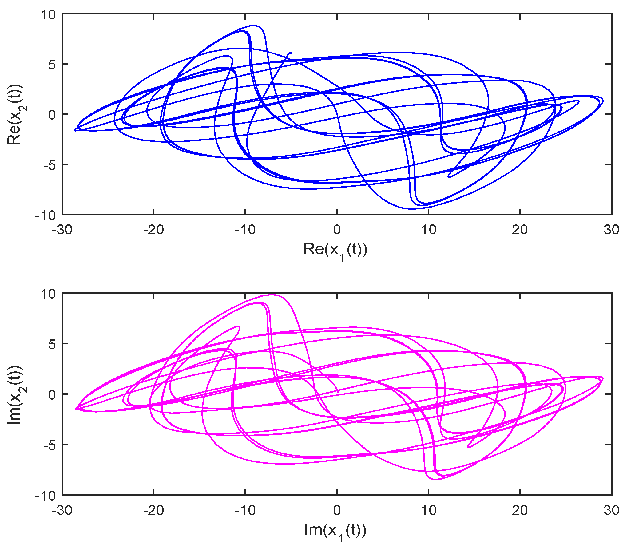
Figure 1.
Bule line stands for transient behavior of variables , and red line stands for transient behavior of variables , of FICVNNs (65).
Figure 1.
Bule line stands for transient behavior of variables , and red line stands for transient behavior of variables , of FICVNNs (65).

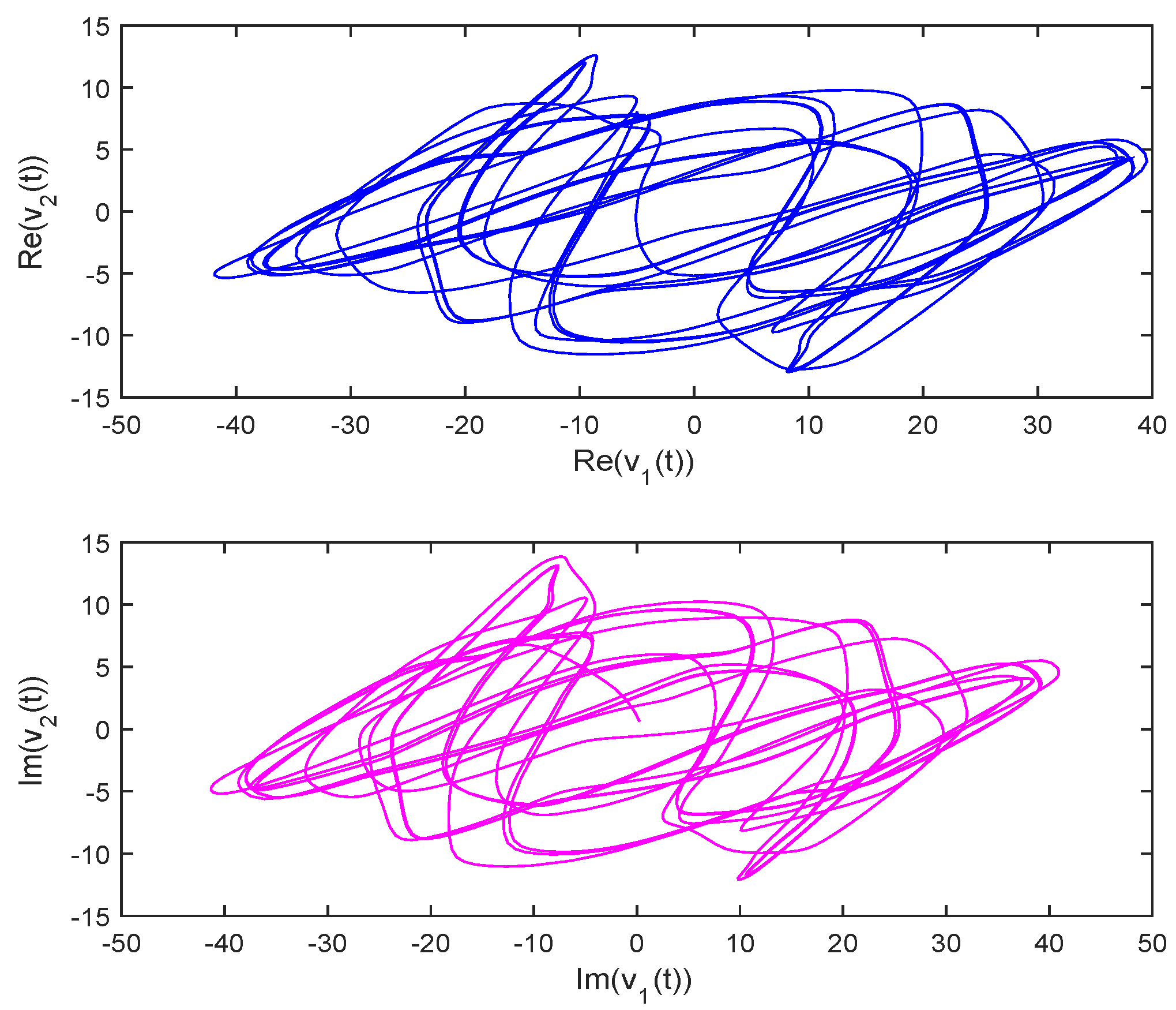
Figure 2.
Bule line stands for transient behavior of variables , and red line stands for transient behavior of variables , of FICVNNs (65).
Figure 2.
Bule line stands for transient behavior of variables , and red line stands for transient behavior of variables , of FICVNNs (65).

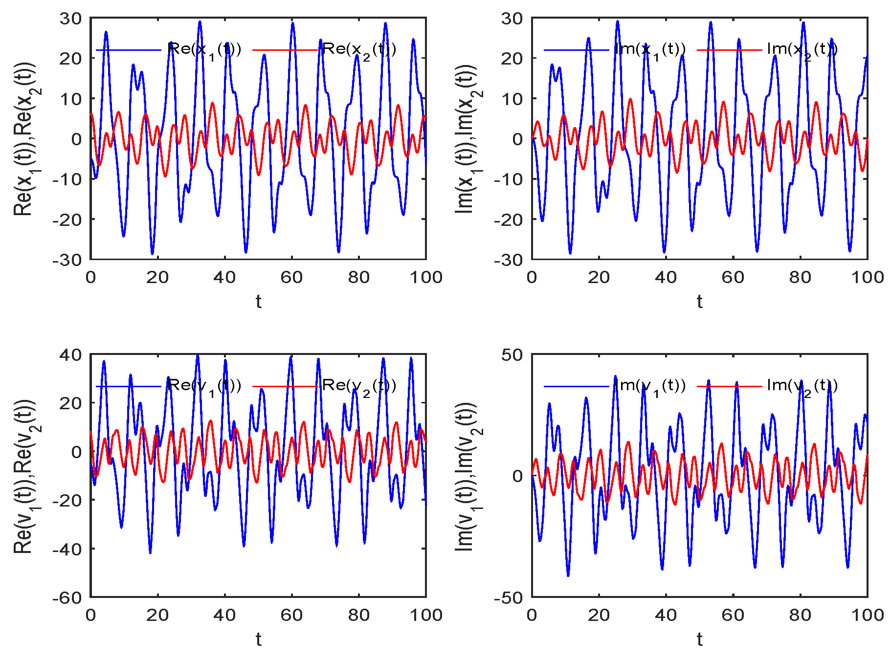
Figure 3.
Bule line stands for state trajectory of variables , , and red line stands for state of trajectory of variables , , of FICVNNs (65) without control.
Figure 3.
Bule line stands for state trajectory of variables , , and red line stands for state of trajectory of variables , , of FICVNNs (65) without control.

Figure 4.
The curves of error states , , external input , and output , under controller (19).

Figure 5.
Trajectory of error states , , under controller (19).

Figure 6.
Trajectories of error with controller .

Figure 7.
The synchronization curve of error states with controller (19).

Figure 8.
PRNG produced by FICVNNs.

Figure 9.
Original signals.

Figure 10.
Encrypted signals.

Disclaimer/Publisher’s Note: The statements, opinions and data contained in all publications are solely those of the individual author(s) and contributor(s) and not of MDPI and/or the editor(s). MDPI and/or the editor(s) disclaim responsibility for any injury to people or property resulting from any ideas, methods, instructions or products referred to in the content. |
© 2024 by the author. Licensee MDPI, Basel, Switzerland. This article is an open access article distributed under the terms and conditions of the Creative Commons Attribution (CC BY) license (https://creativecommons.org/licenses/by/4.0/).
Share and Cite
MDPI and ACS Style
Han, J. Finite-Time Passivity and Synchronization for a Class of Fuzzy Inertial Complex-Valued Neural Networks with Time-Varying Delays. Axioms 2024, 13, 39. https://0-doi-org.brum.beds.ac.uk/10.3390/axioms13010039
AMA Style
Han J. Finite-Time Passivity and Synchronization for a Class of Fuzzy Inertial Complex-Valued Neural Networks with Time-Varying Delays. Axioms. 2024; 13(1):39. https://0-doi-org.brum.beds.ac.uk/10.3390/axioms13010039
Chicago/Turabian StyleHan, Jing. 2024. "Finite-Time Passivity and Synchronization for a Class of Fuzzy Inertial Complex-Valued Neural Networks with Time-Varying Delays" Axioms 13, no. 1: 39. https://0-doi-org.brum.beds.ac.uk/10.3390/axioms13010039
Note that from the first issue of 2016, this journal uses article numbers instead of page numbers. See further details here.