Article

A Statistical Model for Count Data Analysis and Population Size Estimation: Introducing a Mixed Poisson–Lindley Distribution and Its Zero Truncation

by
Gadir Alomair
1,*,
Razik Ridzuan Mohd Tajuddin
2,
Hassan S. Bakouch
3,4 and
Amal Almohisen
5
1
Department of Quantitative Methods, School of Business, King Faisal University, Al Hofuf 31982, Saudi Arabia
2
Department of Mathematical Sciences, Universiti Kebangsaan Malaysia, Bangi 43600, Malaysia
3
Department of Mathematics, College of Science, Qassim University, Buraydah 51452, Saudi Arabia
4
Department of Mathematics, Faculty of Science, Tanta University, Tanta 31111, Egypt
5
Department of Statistics and Operations Research, College of Sciences, King Saud University, Riyadh 11495, Saudi Arabia
*
Author to whom correspondence should be addressed.
Submission received: 25 December 2023 / Revised: 2 February 2024 / Accepted: 12 February 2024 / Published: 17 February 2024
(This article belongs to the Special Issue Methods and Applications of Advanced Statistical Analysis)

Abstract

:
Count data consists of both observed and unobserved events. The analysis of count data often encounters overdispersion, where traditional Poisson models may not be adequate. In this paper, we introduce a tractable one-parameter mixed Poisson distribution, which combines the Poisson distribution with the improved second-degree Lindley distribution. This distribution, called the Poisson-improved second-degree Lindley distribution, is capable of effectively modeling standard count data with overdispersion. However, if the frequency of the unobserved events is unknown, the proposed distribution cannot be directly used to describe the events. To address this limitation, we propose a modification by truncating the distribution to zero. This results in a tractable zero-truncated distribution that encompasses all types of dispersions. Due to the unknown frequency of unobserved events, the population size as a whole becomes unknown and requires estimation. To estimate the population size, we develop a Horvitz–Thompson-like estimator utilizing truncated distribution. Both the untruncated and truncated distributions exhibit desirable statistical properties. The estimators for both distributions, as well as the population size, are asymptotically unbiased and consistent. The current study demonstrates that both the truncated and untruncated distributions adequately explain the considered medical datasets, which are the number of dicentric chromosomes after being exposed to different doses of radiation and the number of positive Salmonella. Moreover, the proposed population size estimator yields reliable estimates.

1. Introduction

Unobserved events in count data are events that were not recorded. For example, the unobserved events in insurance claims refer to the events where the policyholders do not claim. In some cases, even these events are not identified. For example, the number of times a motorist gets stopped by the police. The number of motorists that did not get stopped cannot be identified, which is known as unobserved events. Modeling count data by examining the observed events or both the observed and unobserved events is typical in statistical modeling. This study would like to explore this area by introducing a mixed Poisson–Lindley distribution and extending it to its zero-truncated version, as well as population size estimation.
The Lindley distribution was originally introduced in Bayesian analysis as a mixture of an exponential distribution and a gamma distribution [1]. Ghitany et al. [2] conducted a comprehensive examination of its statistical characteristics. Subsequent research has expanded the Lindley distribution into both two-parameter [3,4,5,6,7,8,9,10,11] and three-parameter variants [12,13,14], each offering innovative enhancements and broader applications. These distributions have been particularly useful in the fields of survival analysis and reliability assessments.
Sankaran [15] pioneered the use of the Lindley distribution as a mixing distribution with the Poisson distribution, thus creating the Poisson–Lindley (PL) distribution. This model, and the methods to estimate its parameters, were studied extensively in later research [16]. Various mixed PL distributions have been proposed as alternatives to the traditional Poisson and negative binomial models for fitting count data [17,18,19]. These new distributions share the overdispersion characteristic common to mixed Poisson distributions [20]. Other notable mixed Poisson models include the Poisson Inverse Pareto distribution [21] and the Poisson-transmuted record-type exponential distribution [22], among others.
When count data exclusively contain positive numbers, zero truncation is a common technique used to adjust distributions accordingly. Examples include the zero-truncated Poisson [23], zero-truncated negative binomial [24], and zero-truncated PL [25] distributions. In fields such as criminology, accurately estimating the size of a population when the frequency of non-events is not observable is a significant challenge [26,27,28,29,30,31,32,33]. Rossmo and Routledge [30] highlighted the necessity of understanding the size of a criminal population to inform the creation of effective laws and policies. Such estimations are still relatively rare in medical research but are equally needed.
The current study aims to introduce a new, practical mixed PL distribution by combining an improved second-degree Lindley (ISDL) distribution [7] with a Poisson variable, resulting in what we name the Poisson-improved second-degree Lindley (PISDL) distribution. This constitutes the first aim of this research. Given the ISDL distribution’s superior modeling performance [7], we anticipate that the PISDL distribution may outperform the original PL distribution. To accommodate strictly positive data, we also introduce a zero-truncated version of the PISDL (ZTPISDL) distribution, which represents the second aim of this research. Furthermore, we propose an innovative estimator for population size in relation to the ZTPISDL distribution, detailed in Section 5.3, marking the third and most original objective of the paper. Understanding the population size is critical for developing comprehensive policies. This study uses data from epidemiology and cytogenetics to demonstrate the applications of the proposed distributions and estimator.
This paper is structured as follows. Section 1 outlines the study’s objectives, building upon previous research on mixed PL distributions, their truncations, and population size estimations. Section 2 presents the PISDL distribution, its statistical properties, and estimation techniques. Section 3 introduces and investigates the zero-truncated PISDL distribution. Section 4 describes the development of a new population size estimator, assuming a PISDL distribution, accompanied by simulation studies in Section 2, Section 3 and Section 4 to evaluate estimator performance. Section 5 applies the proposed models to medical dataset analyses. Finally, Section 6 concludes with a discussion of the implications, limitations, and future research directions of this study.

2. Poisson-Improved Second-Degree Lindley Distribution

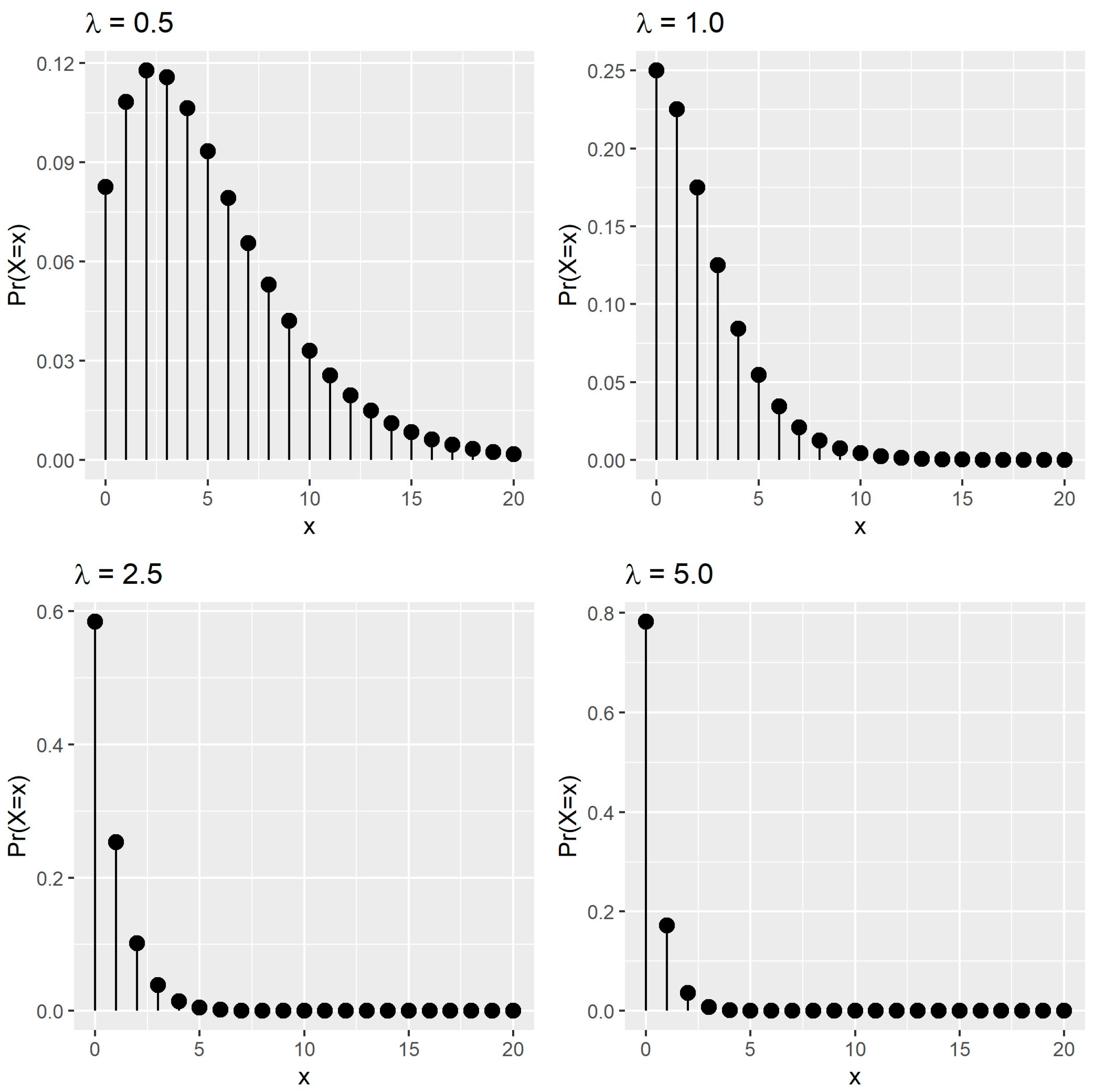
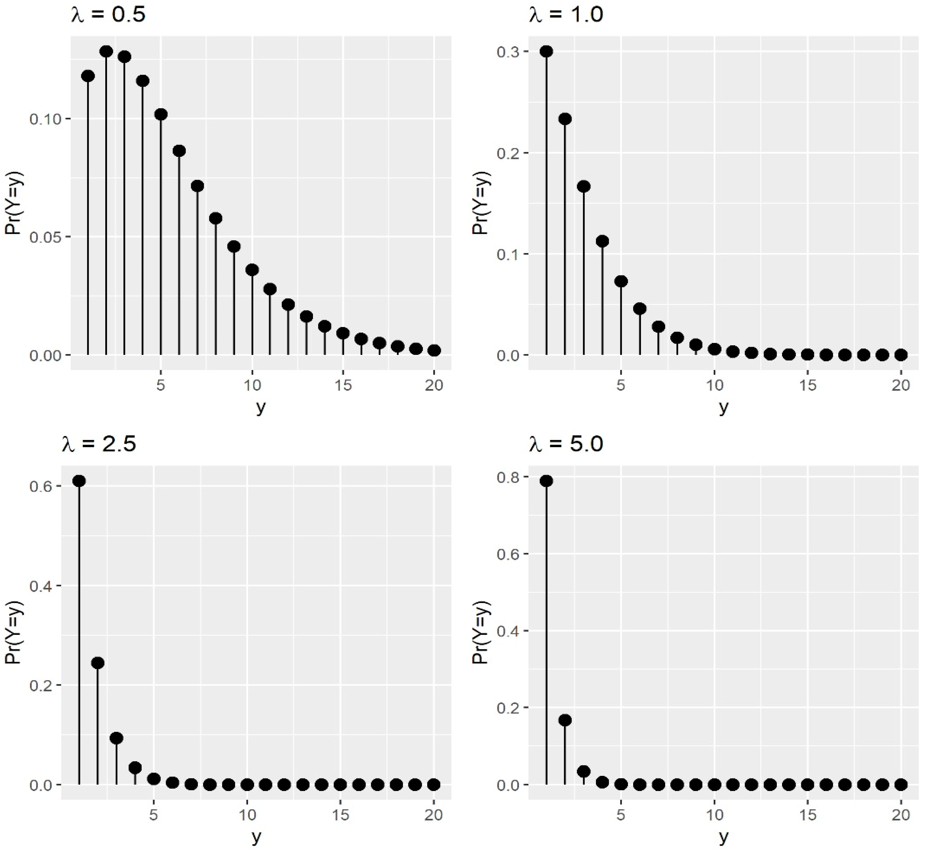
2.1. Probability Mass Function of the PISDL Distribution

Definition 1.
A random variable  X  is said to follow a Poisson-improved second-degree Lindley (PISDL) distribution with parameter θ if it obeys  X | θ ~ P o i s s o n θ  and   θ ~ I S D L λ , where  θ ,   λ > 0 .
Theorem 1.
Let  X  be a random variable that follows PISDL with parameter  λ ; then, the probability mass function (pmf) of  X  is given as
f x = λ 3 λ 2 + 2 λ + 2 x x + 5 + 2 λ x + 2 + λ 2 + 5 λ + 1 x + 3 ;   x = 0 , 1 , 2 , ,   λ > 0 .
Proof. 
Using Definition 1, the pmf of X | θ is
f x | θ = θ x exp θ x ! ;   x = 0 , 1 , 2 , ,   θ > 0 .
The probability density function of θ | λ is
g θ = λ 3 λ 2 + 2 λ + 2 1 + θ 2 exp λ θ ;   λ > 0 , θ > 0 .
The resulting marginal distribution f x   for the PISDL distribution with parameter λ is obtained as follows:
f x = 0 f x | θ g θ d θ = λ 3 λ 2 + 2 λ + 2 x ! 0 θ x 1 + θ 2 exp θ λ + 1 d θ = λ 3 λ 2 + 2 λ + 2 x x + 5 + 2 λ x + 2 + λ 2 + 5 λ + 1 x + 3 .
 □
Figure 1 shows the pmf plot for the PISDL distribution. In Figure 1, the distribution is skewed to the right, unimodal, and decreasing, which is further supported by the decreasing ratio of probability given as
f x + 1 f x = 1 λ + 1 1 + 2 x + λ + 3 x x + 5 + 2 λ x + 2 + λ 2 + 5 .
It is worth noting that the PISDL distribution is actually a three-component mixture distribution that can be written as f x = p 1 f 1 x + p 2 f 2 x + p 3 f 3 x , where f i x is the pmf of the negative binomial distribution with a parameter number of successes i and proportion λ / λ + 1 . When i = 1 , f i x is the pmf of the geometric distribution, which is a special case for the negative binomial distribution. The formulae for p i and f i x for i = 1 , 2 , 3 are given as
p 1 = λ 2 λ 2 + 2 λ + 2 ;   p 2 = 2 λ λ 2 + 2 λ + 2 ;   p 3 = 1 p 1 p 2 ;
f 1 x = λ λ + 1 x + 1 ;   f 2 x = λ 2 x + 1 λ + 1 x + 2 ;   f 3 x = λ 3 x + 1 x + 2 2 λ + 1 x + 3 .
Even though the PISDL distribution is a three-component mixture negative binomial distribution, the existence of three modes cannot be seen in any of the plots in Figure 1 for the selected values of λ . This insinuates that the three modes, which come from the three sub-populations, must be located very close to each other. As mentioned in [34], if the modes of the sub-populations are located very close to each other, then the population will have a single mode. As such, if the existence of the modes of the sub-populations, each with very close mode values, can be certain, then this distribution can be considered as one of the candidates for model fittings.
The cumulative distribution function (cdf) for the PISDL distribution is given in Equation (2) and visualized in Figure 2. In Figure 2, it is clear that the PISDL distribution has a valid cdf since F x 1 as x .
F x = 1 λ 4 + 2 λ 3 x + 3 + λ 2 x 2 + 7 x + 13 + 2 λ x + 4 + 2 λ 2 + 2 λ + 2 λ + 1 x + 3 .
Based on Equation (2), the survival function S x can be obtained and given as
S x = λ 4 + 2 λ 3 x + 3 + λ 2 x 2 + 7 x + 13 + 2 λ x + 4 + 2 λ 2 + 2 λ + 2 λ + 1 x + 3 .
The plot for the survival function of the PISDL distribution is given in Figure 3.
The hazard rate function h x is defined by taking the ratio of the pmf to the survival function, i.e., h x = f x / S x , and is given as
h x = λ 3 x x + 5 + 2 λ x + 2 + λ 2 + 5 λ 4 + 2 λ 3 x + 3 + λ 2 x 2 + 7 x + 13 + 2 λ x + 4 + 2 .
The hazard rate function plot is given in Figure 4. In Figure 4, it can be noted that the hazard rate functions show an increasing pattern with a limiting value of λ , meaning lim x h x = λ .

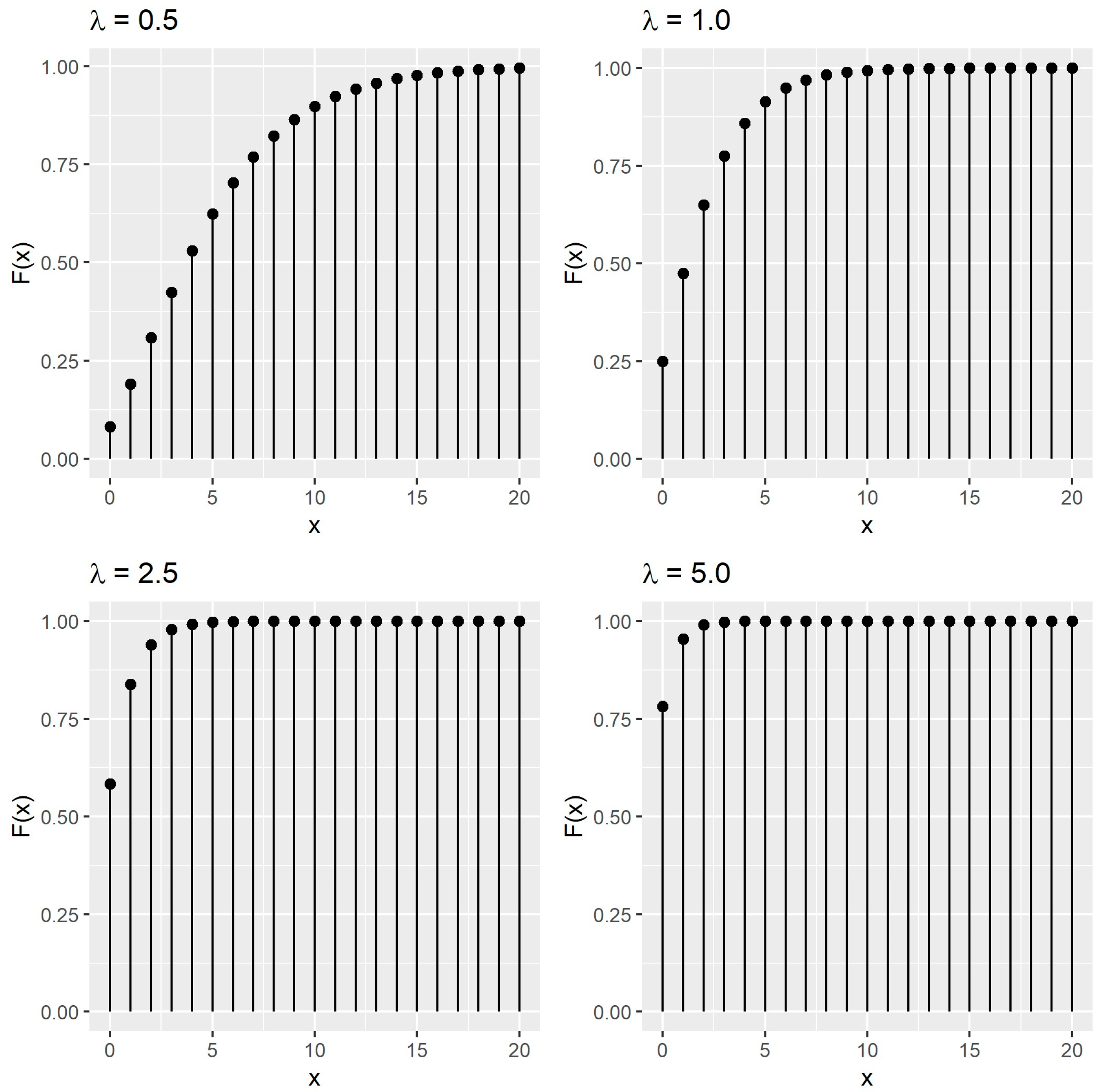
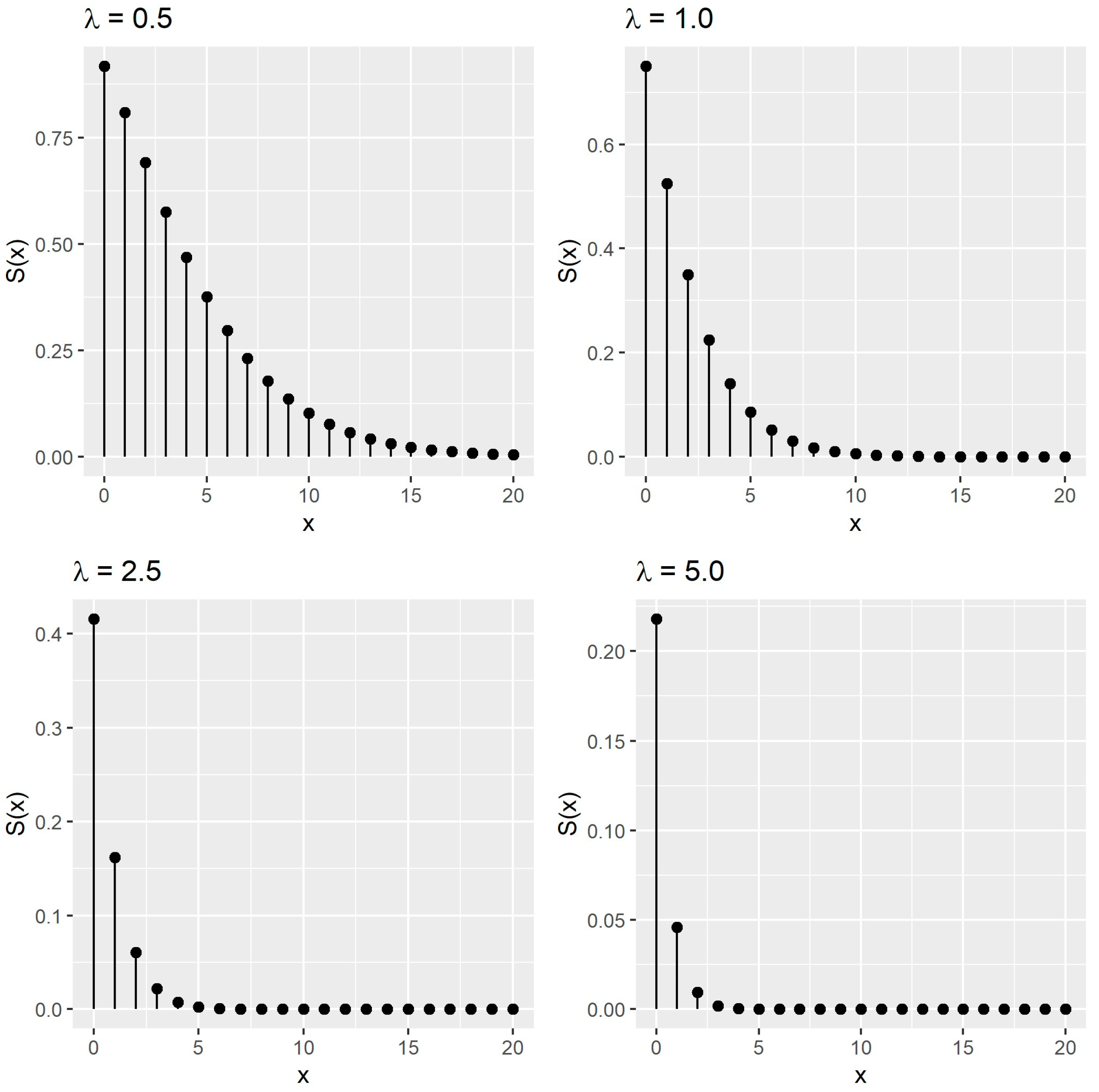
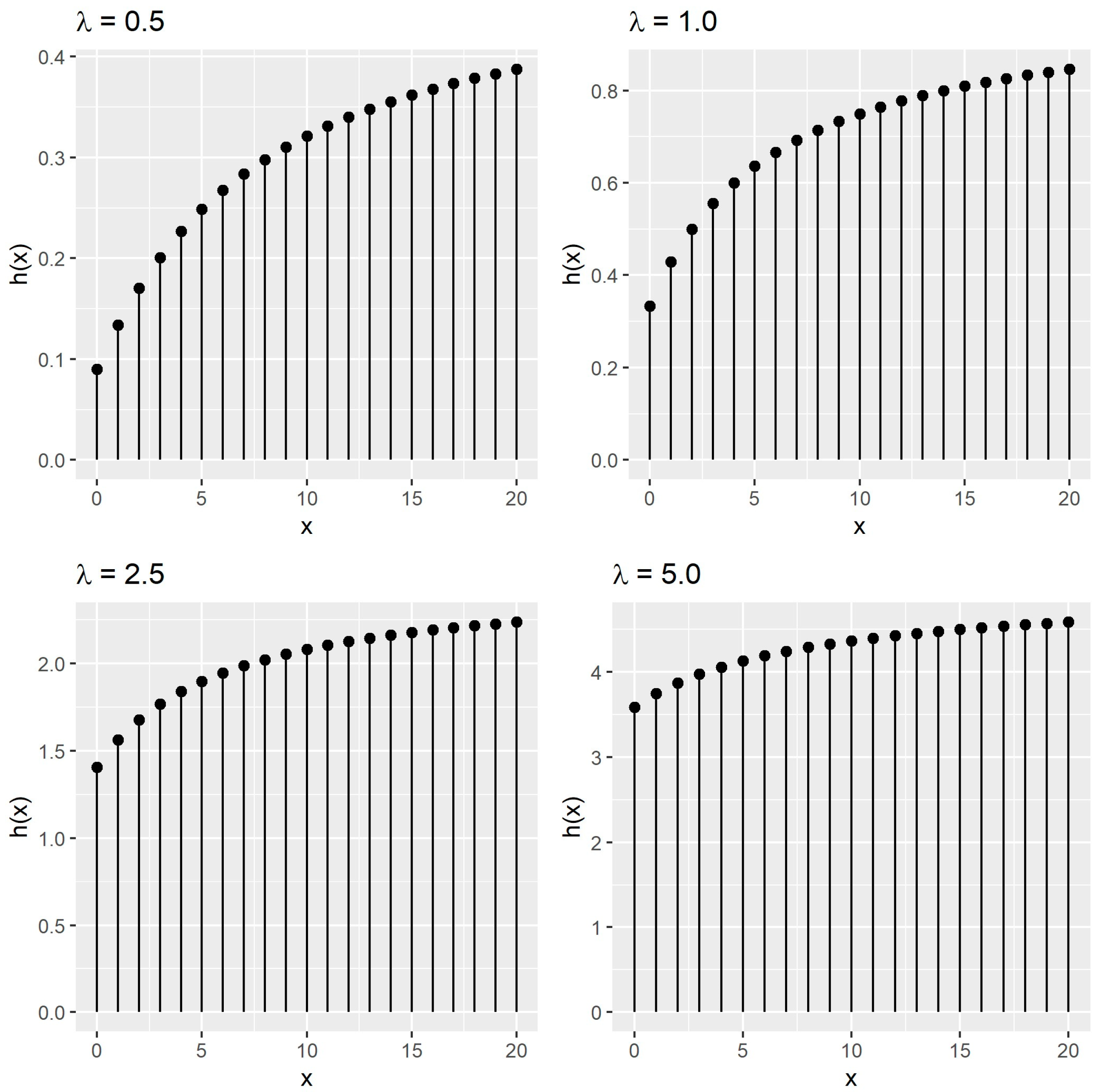
2.2. Some Statistical Properties of the PISDL Distribution

The k t h moment in the origin of the PISDL distribution can be written by the following generic expression:
E X k = x = 0 x k f x .
In particular, the first two moments in the origin using Equation (5) are obtained, respectively, as
E X = λ 2 + 4 λ + 6 λ λ 2 + 2 λ + 2 ,   E X 2 = λ + 2 λ 2 + 4 λ + 6 + 4 λ + 3 λ 2 λ 2 + 2 λ + 2 .
Hence, the index of dispersion ( I O D X ) can be written as
I O D X = V a r X E X = E X 2 E X 2 E X = E X 2 E X E X = 1 + 1 λ λ 4 + 2 4 λ 3 + 12 λ 2 + 12 λ + 6 λ 4 + 6 λ 3 + 16 λ 2 + 20 λ + 12 .
Since the I O D X > 1 , the PISDL distribution is overdispersed for all λ .
The mode of the PISDL distribution can be obtained by maximizing the log pmf of the PISDL distribution or equivalently by solving the quadratic equation A x m 2 + B x m + C = 0 , where x m 0 is the mode of the distribution, where A = ln λ + 1 , B = 2 λ + 5 ln λ + 1 2 , and C = 5 + λ λ + 4 ln λ + 1 2 λ 5 . As a result, the solution for the equation is
x m = 2 5 + 2 λ ln 1 + λ + 4 + 5 + 4 λ ln 1 + λ 2 2 ln 1 + λ .
It can be shown from Figure 1 that x m > 0 , for 0 < λ < 1   and when λ 1 , then x m = 0 . The moment, the probability and the cumulant generating functions are given, respectively, is
M X t = λ 3 λ 2 + 2 λ + 2 s + 2 s 2 + 2 s 3 ;   s = s t = λ + 1 exp t 1 ,
G X t = λ 3 λ 2 + 2 λ + 2 r + 2 r 2 + 2 r 3 ;   r = s ln t = λ + 1 t 1 ,
C X t = ln M X t = 3 ln λ ln λ 2 + 2 λ + 2 + ln s + 2 s 2 + 2 s 3 .

2.3. Parameter Estimation of the PISDL Distribution

The parameter of the PISDL distribution needs to be estimated before modeling real-world datasets. Here, parameter estimation is based on the two commonly used estimation methods, which are the methods of moments and maximum likelihood.

2.3.1. Method of Moments Estimator

The method of moments estimator can be obtained by equating the sample mean to the population mean. Therefore, the moment estimator of λ , hereby denoted as λ ~ ,   can be obtained by solving the following equation:
x ¯ = λ ~ 2 + 4 λ ~ + 6 λ ~ λ ~ 2 + 2 λ ~ + 2 ,
or equivalently solving the cubic equation A λ ~ 3 + B λ ~ 2 + C λ ~ + D = 0 , where A = x ¯ , B = 2 x ¯ 1 , C = 2 x ¯ 4 , and D = 6 .

2.3.2. Maximum Likelihood Estimator

Note that the log-likelihood function can be written as   l = ln L = i = 1 n ln f x i = x = 0 n x ln f x , where n x is the frequency of x-valued data. Hence, l is given as
l = 3 n ln λ n ln λ 2 + 2 λ + 2 n x ¯ + 3 ln λ + 1 + x = 0 n x ln x x + 5 + 2 λ x + 2 + λ 2 + 5 .
By differentiating l with respect to λ , we obtain
d l d λ = 3 n λ 2 n λ + 1 λ 2 + 2 λ + 2 n x ¯ + 3 λ + 1 + x = 0 n x 2 λ + x + 2 x x + 5 + 2 λ x + 2 + λ 2 + 5 ,
in which equating it to zero and solving it yields the maximum likelihood estimator (MLE) for λ , which is abbreviated as   λ ^ . Equivalently, one can directly maximize the l to obtain a similar result. To estimate the variance of λ ^ , Fisher’s information about λ and I λ needs to be obtained, and it is given as
I λ = 4 λ 6 + 7 λ 5 7 λ 4 40 λ 3 52 λ 2 36 λ 12 λ 2 λ + 1 2 λ 2 + 2 λ + 2 2 + 4 λ 3 λ + 1 3 λ 2 + 2 λ + 2 x = 0 λ + x + 2 2 x x + 5 + 2 λ x + 2 + λ 2 + 5 λ + 1 x .
The summation term cannot be written in a closed form, but one may use several Lerch Transcendent [35] functions for it. However, it is only practical to leave the summation term as is. So, the variance of λ ^ can be written as I 1 λ / n and, subsequently, the 1 α 100 % confidence interval can be written as λ ^ z α I 1 / 2 λ / n . If α = 0.025 , and then the 95% confidence interval will be obtained. The summation term reduces considerably to a simple form when λ ^ is substituted, thus resulting in a constant. This will eventually give an estimated variance of λ ^ . For example, for n = 100 and when λ ^ = 1.8793, the summation equates to 1.4284, which then results in the estimated variance of 0.0145.

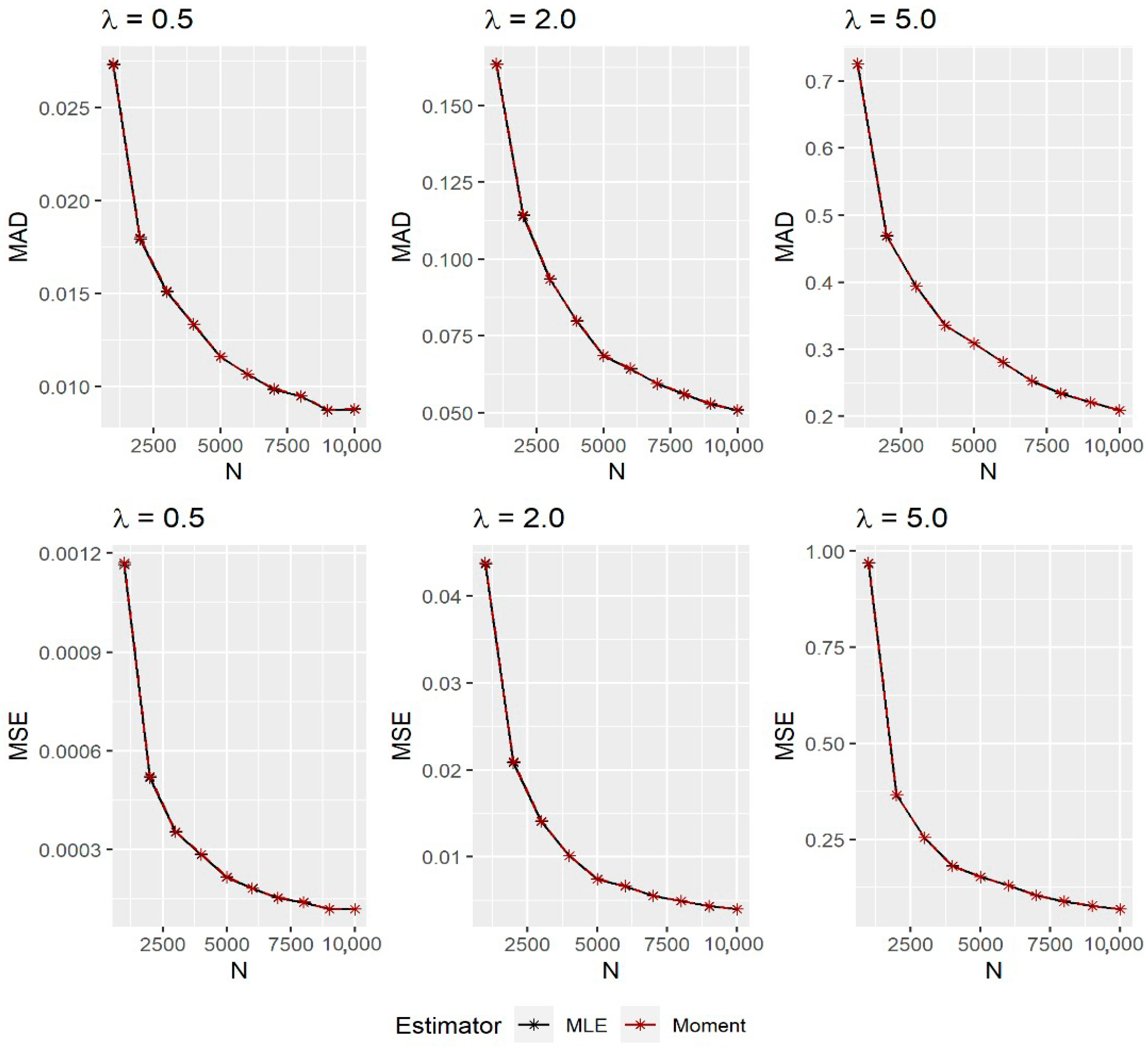
2.4. Simulation Study

A simulation study is conducted to assess the performance of the two earlier estimators in estimating the parameter of the PISDL distribution. The algorithm for the simulation study is as follows:
Step 1:
Generate N = 1000 ,   2000 ,   ,   10,000   random data that follows the PISDL distribution with λ = 0.5 .
Step 2:
Obtain the estimated λ using MLE and moment estimator.
Step 3:
Repeat Steps 1–2 for a total of 2000 iterations and obtain the estimates.
Step 4:
Calculate the mean absolute deviation, MAD, and the mean squared error values, MSEs, given, respectively, as M A D = i = 1 2000 λ ˇ λ / 2000 and M S E = i = 1 2000 λ ˇ λ 2 / 2000 , where λ ˇ can be the MLE or moment estimator for λ .
Step 5:
Repeat Steps 3–4 for λ = 2.0 ,   5.0 .
Generally, if the MAD and MSE approach zero as N increases, then the estimate is asymptotically unbiased and consistent. For the simulation study, R software version 3.0.2 is used, and the estimated parameter using MLE is obtained using the optim command to optimize the log-likelihood value. The results of the simulation study are presented in Figure 5. In Figure 5, for any value of λ , as N increases, the MAD and the MSE of the MLE and the moment estimator decrease, suggesting that both estimates are asymptotically unbiased and consistent.

3. Zero-Truncated Poisson-Improved Second-Degree Lindley Distribution

Truncation is a widely used trait in real-world situations in a variety of domains, including industry [23,24,25], medicine [23,24], and many more. The progression of a disease that is not an increasing function but will stabilize after a certain period is an example of truncation. Therefore, a flexible truncated count data distribution is introduced by truncating the PISDL distribution at zero, yielding a zero-truncated Poisson-improved second-degree Lindley distribution (ZTPISDL). It was observed that the PISDL and the PL distributions are equally competent based on the two datasets considered in Section 5. Therefore, it is expected that the ZTPISDL distribution to be as competent as the zero-truncated PL (ZTPL) distribution. The development and the statistical properties of the ZTPISDL distribution are discussed in the following sections.

3.1. Probability Mass Function of the ZTPISDL Distribution

Definition 2.
A random variable Y is said to follow a ZTPISDL distribution if it obeys  X | λ ~ P I S D L λ    and  p y = f y / 1 f 0 , where p(y) is the pmf of Y.
Theorem 2.
Let Y be a random variable that follows the ZTPISDL with parameter  λ , and then the pmf of Y is given as
p y = λ 3 λ 4 + 6 λ 3 + 13 λ 2 + 8 λ + 2 y y + 5 + 2 λ y + 2 + λ 2 + 5 λ + 1 y ,   y = 1 , 2 , 3 ,
Proof. 
Using Definition 2, the pmf of Y is obtained. □
Figure 6 shows the pmf plot for the ZTPISDL distribution that follows similar shapes as the pmf plot for the PISDL distribution, which is skewed to the right, unimodal, and decreasing. Using the log of p y defined in (10), the mode y m o d of the distribution can be obtained by solving the following formula:
y mod = D + D 2 4 A E 2 A ,
where A = ln λ + 1 ,   D = A 2 λ + 5 2 , and E = A λ 2 + 4 λ + 5 2 λ 5 .

3.2. Some Statistical Properties of the ZTPISDL Distribution

If Y ~ Z T P I S D L for y = 1 ,   2 ,   3 ,   , then the k t h   moment for Y can be easily obtained because it satisfies E Y k = E X k / 1 f 0 . The first two moments in the origin are obtained and can be, respectively, written as
E Y = λ + 1 3 λ 2 + 4 λ + 6 λ λ 4 + 6 λ 3 + 13 λ 2 + 8 λ + 2 , E Y 2 = 1 + λ 3 λ + 2 λ 2 + 4 λ + 6 + 4 3 + λ λ 2 2 + λ 1 + λ 8 + λ 5 + λ .
Using a similar approach as the I O D X   for X, the index of dispersion for Y ( I O D Y ) can be written as
I O D Y = V a r Y E Y = 1 λ 2 2 + λ 6 + λ 4 + λ + 4 + 2 λ 8 + λ 5 + λ 2 + λ 1 + λ 8 + λ 5 + λ .
Based on the I O D Y , the ZTPISDL distribution is underdispersed (overdispersed) when λ > < 1.51494 . The ZTPISDL distribution is only equidispersed when λ = 1.51494 . The recurrence probability for Y is similar for X, except the x is substituted with y because
p y + 1 p y = f y + 1 / 1 f 0 f y / 1 f 0 = f y + 1 f y .
The generating functions for both ZTPISDL and PISDL distributions can be related since their pmfs are related as well. Therefore, their relationships are given, respectively, below so that the moment generating, the cumulant generating, and the probability generating functions for Y can be worked out as follows:
M Y t = M X t f 0 1 f 0 ,
C Y t = ln M Y t = ln M X t f 0 ln 1 f 0 ,
G Y t = M Y ln t = M X ln t f 0 1 f 0 = G X t f 0 1 f 0 .

3.3. Parameter Estimation of the ZTPISDL Distribution

The parameter of the ZTPISDL distribution can be estimated using the moment and MLE techniques. The moment estimator of λ , hereby denoted as λ ~ , can be obtained by solving the following equation:
y ¯ = λ ~ + 1 3 λ ~ 2 + 4 λ ~ + 6 λ ~ λ ~ 4 + 6 λ ~ 3 + 13 λ ~ 2 + 8 λ ~ + 2 ,
or equivalently solving the quintic equation A λ ~ 5 + B λ ~ 4 + C λ ~ 3 + D λ ~ 2 + E λ ~ + F = 0 , such that A = 1 y ¯ , B = 7 6 y ¯ , C = 21 13 y ¯ , D = 31 8 y ¯ , E = 22 2 y ¯ , and F = 6 . For MLE, the log-likelihood function l is given as
l = 3 n ln λ n ln λ 4 + 6 λ 3 + 13 λ 2 + 8 λ + 2 n y ¯ ln λ + 1 + y = 1 n y ln y y + 5 + 2 λ y + 2 + λ 2 + 5 .
By differentiating l with respect to λ , we obtain
d l d λ = 3 n λ n 4 λ 3 + 18 λ 2 + 26 λ + 8 λ 4 + 6 λ 3 + 13 λ 2 + 8 λ + 2 n y ¯ λ + 1 + y = 1 n y 2 λ + y + 2 y y + 5 + 2 λ y + 2 + λ 2 + 5 ,
in which equating it to zero and solving it implies the MLE for λ , which is denoted as λ ^ . Equivalently, one can directly maximize the l directly to obtain a similar result.

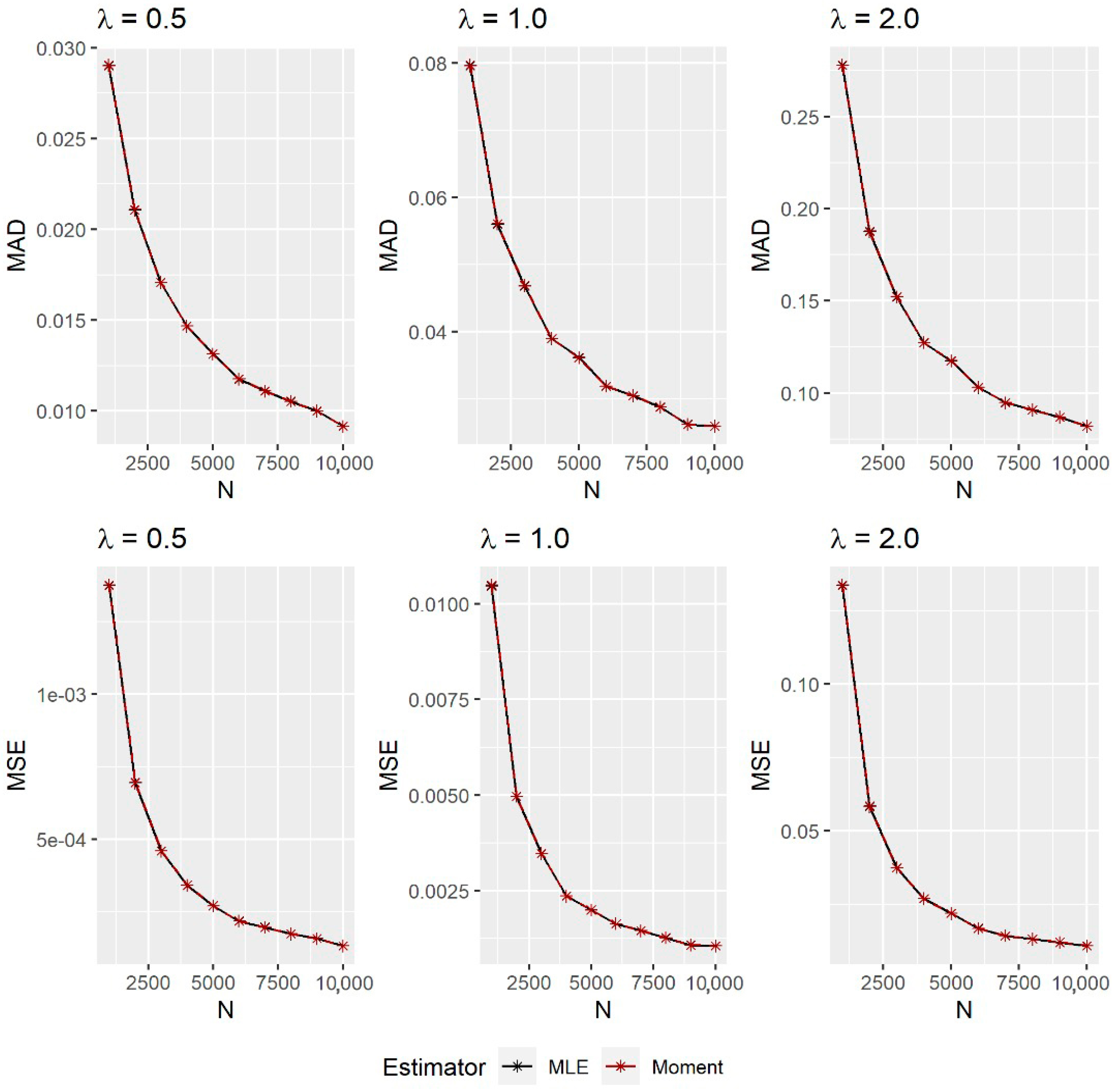
3.4. Simulation Study

A simulation study is conducted to assess the performance of the obtained estimators for the parameter of the ZTPISDL distribution. The algorithm for the simulation study is similar to the one in Section 2.4, except that the data are generated using the ZTPISDL distribution. Similarly, R software is used, and the estimated parameter using MLE is obtained using the optim command to optimize the log-likelihood value. The findings of the simulation study are shown in Figure 7. Figure 7 shows that for any value of λ , as N increases, the MAD and the MSE of both estimates fall, indicating that they are both asymptotically unbiased and consistent.
When dealing with a truncated distribution, the population size is usually unknown and needs to be estimated. Assuming that a population follows the ZTPISDL distribution, a population size estimator is developed and studied. The discussion on the population size is provided in the next section.

4. Population Size Estimation

4.1. Horvitz–Thompson Estimator under ZTPISDL Distribution (HT-ZTPISDL)

A popular estimator for the population size is the Horvitz–Thompson estimator [36], which includes information from both truncated and untruncated distributions. A Horvitz–Thompson estimator has the following form:
N ^ = n 1 Pr X = 0 | ω ^ ,
where ω ^ is the estimator for ω for a distribution and n is the sample size. Basically, the estimated parameter of the truncated distribution is substituted into the probability mass function of the untruncated distribution for the unobserved events. The estimator for the population size   N ^ , which follows a ZTPISDL distribution in the form of the Horvitz–Thompson estimator (HT-ZTPISDL), is given as
N ^ = n λ ^ + 1 3 λ ^ 2 + 2 λ ^ + 2 λ ^ 4 + 6 λ ^ 3 + 13 λ ^ 2 + 8 λ ^ + 2 ,
where λ ^ is the MLE for λ in the ZTPISDL distribution.

4.2. Variance and Confidence Interval for HT-ZTPISDL

Böhning [37] has provided a simple yet informative method for obtaining a variance for any population size estimator using the conditional expectation technique. The variance of HT-ZTPISDL can be written as
V a r N ^ = V a r λ ^ , n n g λ ^ = V a r n E λ ^ | n n g λ ^ + E n V a r λ ^ | n n g λ ^ ,
where g λ = 1 f 0 . Observe that the variation in estimating the population size comes from two sources of variation. The first term in Equation (14) explains the binomial variation involved in sampling n units of data with population size N and probability g λ [37]. The second term in Equation (14) explains the variation that occurs when estimating parameter λ using n observed data [37]. Using the delta method for the first term of Equation (14), we obtain
E λ ^ | n n g λ ^ = n g λ .
As n ~ b i n o m i a l N , g λ , we obtain
V a r n E λ ^ | n n g λ ^ = V a r n n g λ = N g λ 1 g λ g λ 2 .
The equation above is further estimated by substituting N g λ   with n and   λ with λ ^ , yielding
V a r ^ n E λ ^ | n n g λ ^ n 1 g λ ^ g λ ^ 2 .
For the ZTPISDL distribution, we obtain
g λ = λ 4 + 6 λ 3 + 13 λ 2 + 8 λ + 2 λ + 1 3 λ 2 + 2 λ + 2 .
Therefore,
V a r ^ n E λ ^ | n n g λ ^ n λ ^ 3 λ ^ + 1 3 λ ^ 2 + 2 λ ^ + 2 λ ^ 2 + 4 λ ^ + 5 λ ^ 4 + 6 λ ^ 3 + 13 λ ^ 2 + 8 λ ^ + 2 2 .
Now, consider the second term of Equation (14), and assume that
E n V a r λ ^ | n n g λ ^ V a r λ ^ | n n g λ ^ .
Using the delta method, we obtain
V a r λ ^ | n n g λ ^ = n 2 V a r λ ^ | n 1 g λ ^ n 2 g λ g λ 2 2 V a r λ ^ ,
where V a r λ ^ = I 1 λ / n and I λ   is given in Equation (9). Therefore,
V a r λ ^ | n n g λ ^ = n λ 4 λ + 1 4 λ 4 + 10 λ 3 + 37 λ 2 + 52 λ + 30 2 λ 4 + 6 λ 3 + 13 λ 2 + 8 λ + 2 4 I 1 λ .
By substituting λ with λ ^ , the second term of Equation (14) can be estimated as
E ^ n V a r λ ^ | n n g λ ^ = n λ ^ 4 λ ^ + 1 4 λ ^ 4 + 10 λ ^ 3 + 37 λ ^ 2 + 52 λ ^ + 30 2 λ ^ 4 + 6 λ ^ 3 + 13 λ ^ 2 + 8 λ ^ + 2 4 I 1 λ ^ .
By combining Equations (15) and (16), the variance of the HT-ZTPISDL can be estimated as
V a r ^ N ^ = n λ ^ 3 λ ^ + 1 3 λ ^ 2 + 2 λ ^ + 2 λ ^ 2 + 4 λ ^ + 5 λ ^ 4 + 6 λ ^ 3 + 13 λ ^ 2 + 8 λ ^ + 2 2 + n λ ^ 4 λ ^ + 1 4 λ ^ 4 + 10 λ ^ 3 + 37 λ ^ 2 + 52 λ ^ + 30 2 λ ^ 4 + 6 λ ^ 3 + 13 λ ^ 2 + 8 λ ^ + 2 4 I 1 λ ^ .
Therefore, the 95% confidence interval for the estimator can be written as N ^ z 0.025 V a r ^ N ^ , where z 0.025 = 1.96 .

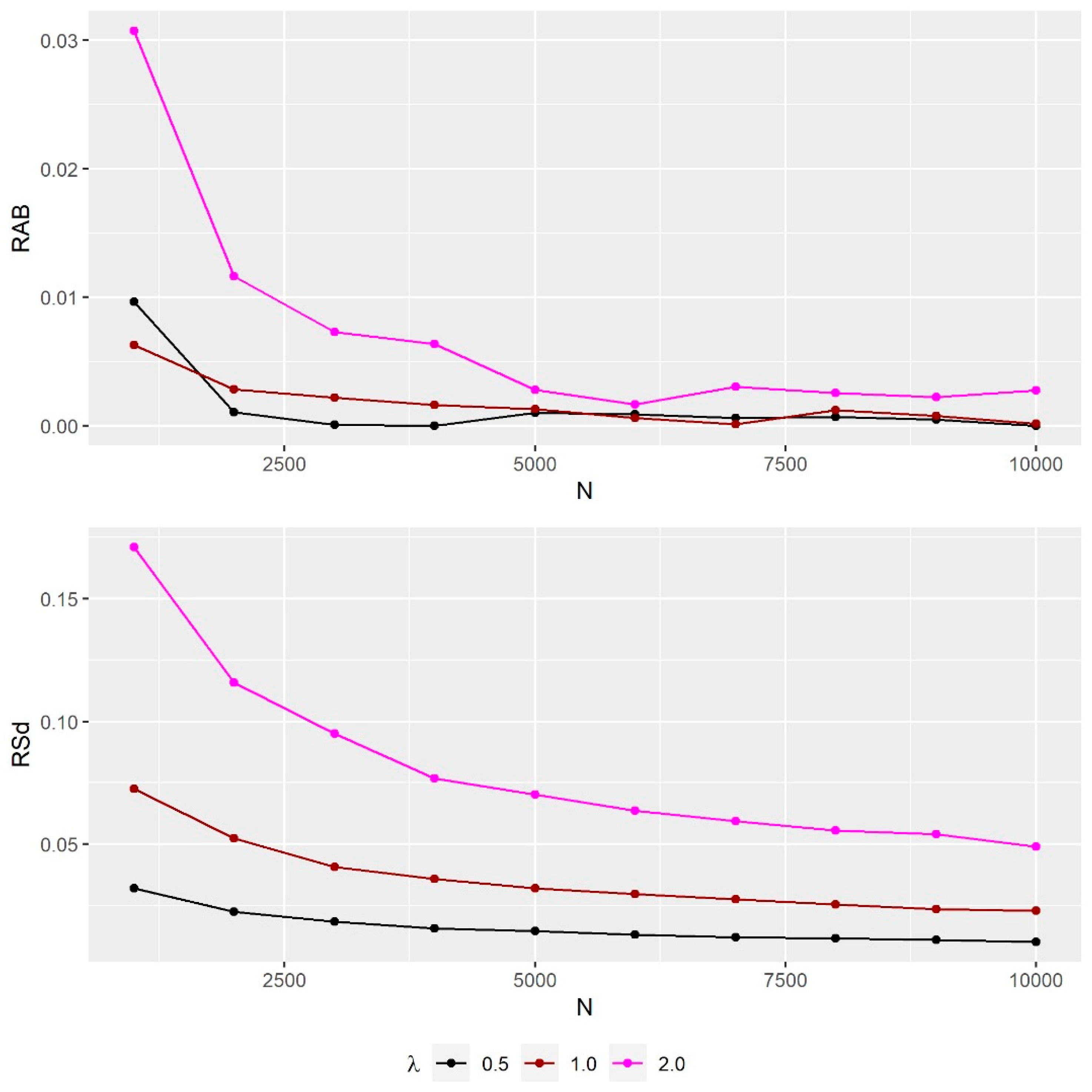
4.3. Simulation Study

A simulation study is conducted to assess the performance of the HT-ZTPISDL estimator in estimating the population size when the data are generated from the ZTPISDL distribution. The algorithm for the simulation study is as follows:
Step 1:
Generate N = 1000 ,   2000 ,   ,   10 , 000   random data, which follow the ZTPISDL distribution with λ = 0.5 .
Step 2:
Obtain λ ^ using the MLE and use λ ^ to obtain N ^ .
Step 3:
Repeat Steps 1–2 for a total of 2000 iterations and obtain the estimates.
Step 4:
Calculate the relative absolute error, RAB values, and the relative standard deviation, RSd values, given, respectively, as R A B = N ^ ¯ N / N and R S d = 1 N i = 1 2000 N ^ N ^ ¯ 2 / 2000 , where N ^ ¯ = i = 1 2000 N ^ / 2000 .
Step 5:
Repeat Steps 3–4 for λ = 2.0 ,   5.0 .
R software is used to obtain λ ^ using the optim command, and N ^ is obtained by plugging in λ ^ in Equation (10). The results of the simulation study are presented in Figure 8. In this figure, for any value of λ , as N increases, the MAD and the MSE of N ^ decreases, suggesting that N ^ is asymptotically unbiased and consistent.

5. Medical Data Applications

The applications in the medical datasets are segregated into three subsections with respect to the PISDL distribution, the ZTPISDL distribution, and the estimation of the population size. For a comparison of the model fittings, Akaike’s information criterion, AIC [38], and Bayesian information criterion, BIC [39], are used.

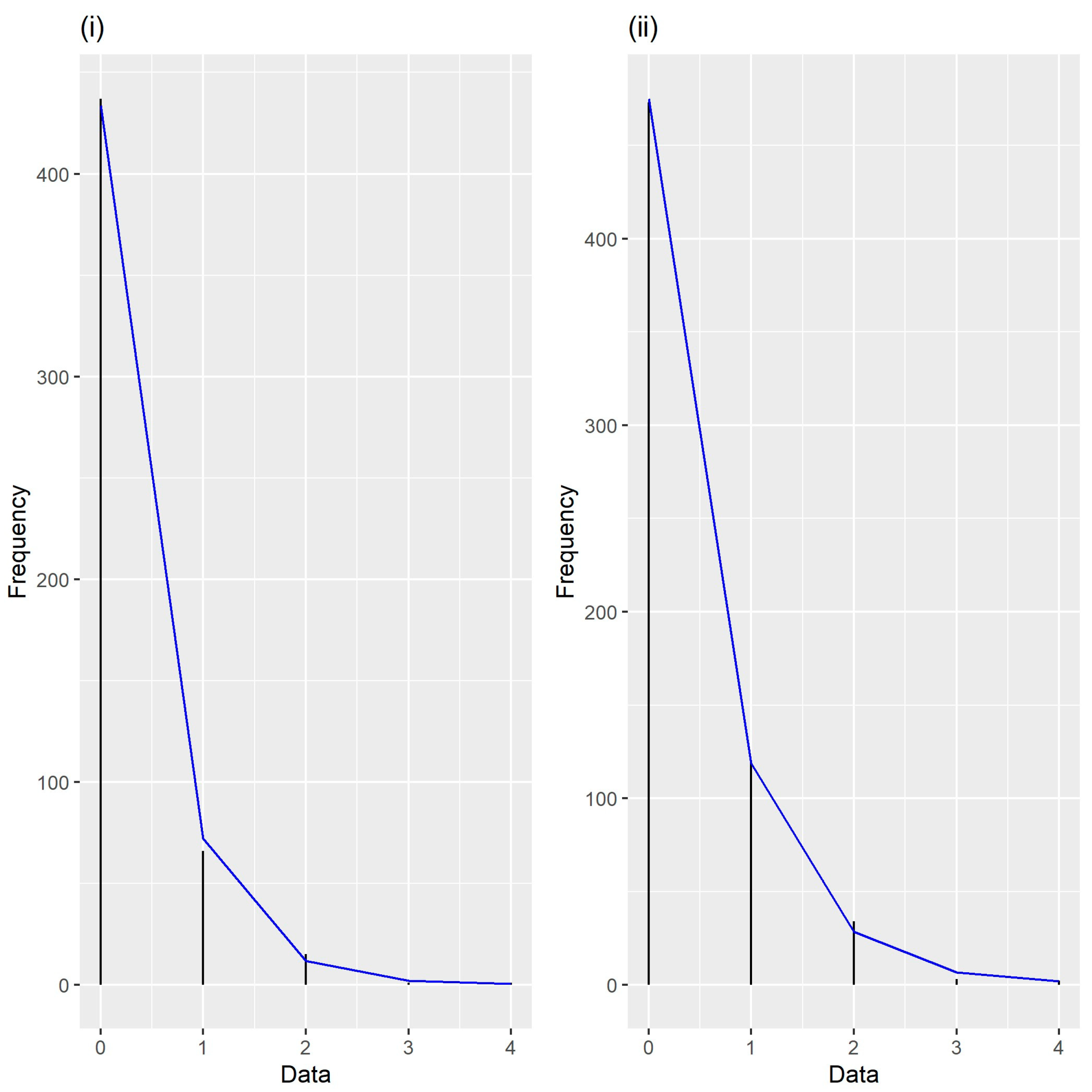
5.1. Model Fittings Using the PISDL Distribution

Two datasets on the number of dicentric chromosomes after being exposed to different doses of radiation (0.405 and 0.600) that were studied by Puig and Barquinero [40] are considered in fitting using the PISDL distribution. The two datasets are overdispersed with dispersion values of 1.2704 and 1.2178, respectively. Since the PISDL distribution is closely related to the Poisson and the PL distributions, the model fittings from the PISDL distribution are compared with those from the Poisson and the PL distributions. The results of the model fittings for the two datasets using the three distributions are summarized in Table 1 and Table 2.
In both tables, the Poisson distribution does not fit the data based on the p-value. On the other hand, the model fittings based on both PL and PISDL distributions gave similar AIC and BIC values, as well as non-significant p-values, indicating that both distributions can be used for describing the number of dicentric chromosomes after being exposed to radiation of different doses. However, the first dataset was fitted better by the PL distribution, whereas the second dataset was fitted better by the PISDL distribution. Therefore, it is reasonable to suggest that both PL and PISDL distributions are equally competent and can be selected as the best distributions in explaining the number of dicentric chromosomes after being exposed to two different doses of radiation.
The comparison between the empirical plots of the data and the fitted values based on Equation (1) in Theorem 1 for the considered datasets, (i) the number of dicentric chromosomes after being exposed to a 0.405 radiation dose, and (ii) the number of dicentric chromosomes after being exposed to a 0.600 radiation dose are presented in Figure 9.

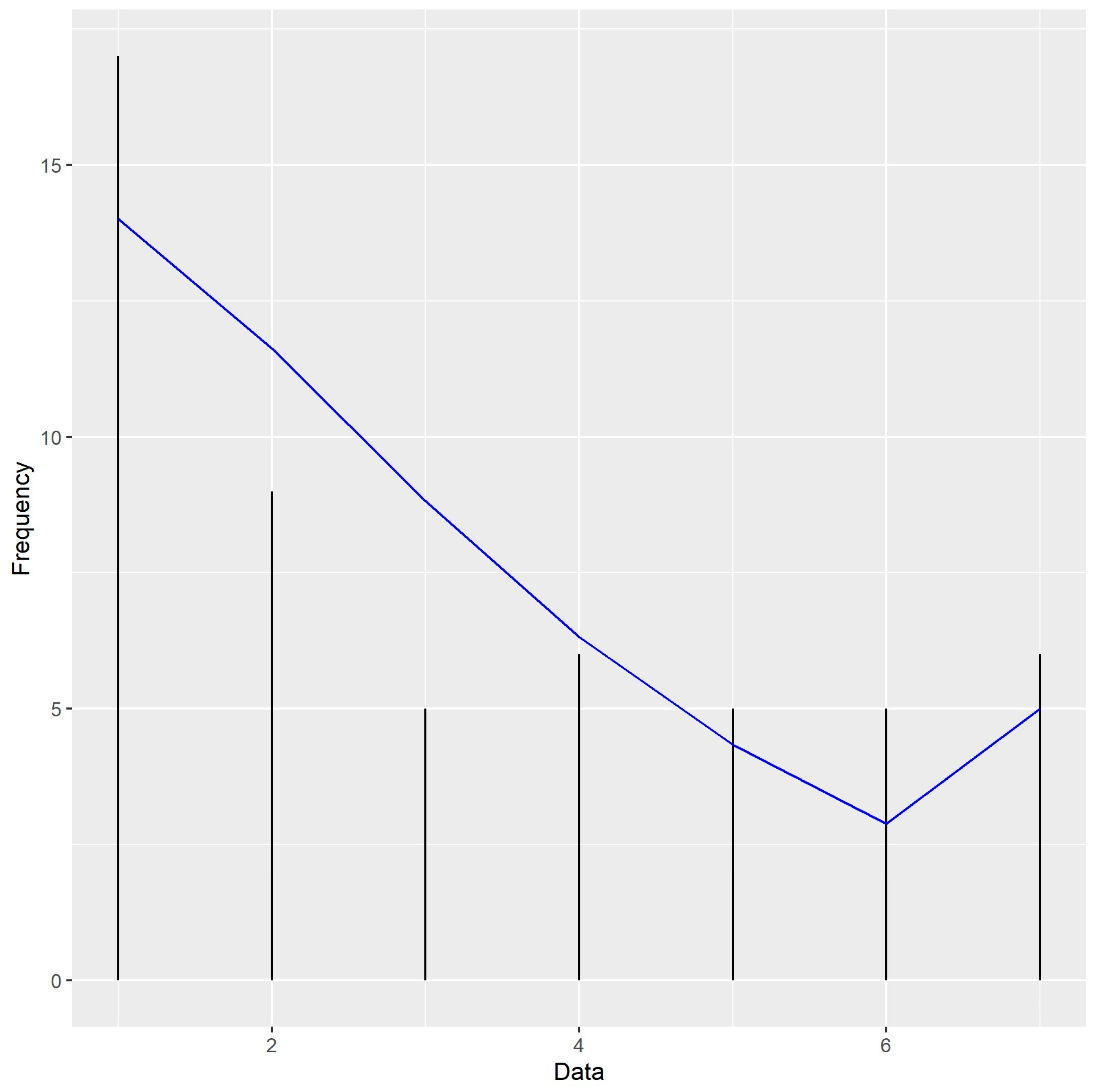
5.2. Model Fittings Using ZTPISDL Distribution

A dataset on the number of positive samples of Salmonella data, which was initially given in a survey study by Snow et al. [41] and later summarized by Arnold et al. [42], is considered in model fitting using the zero-truncated Poisson (ZTP), the zero-truncated PL (ZTPL), and the ZTPISDL distributions. The data refer to the number of farms with at least one positive sample of Salmonella. The dataset is overdispersed with a dispersion value of 1.4381. The results of the model fittings are given in Table 3.
In Table 3, the ZTP distribution does not provide a good fit to the data based on the p-value. On the contrary, the ZTPISDL and the ZTPL distributions provide a good fit to the data based on the AIC and BIC values, as well as the non-significant p-value. However, the dataset was fitted better by the ZTPISDL distribution. Therefore, this suggests that the ZTPISDL is the best distribution in describing the number of positive samples of Salmonella data. The comparison between the empirical plots of the data and the fitted value based on Equation (10) in Theorem 2 for the above dataset is presented in Figure 10.

5.3. Estimating Population Size

The dataset studied in Section 5.2 on the number of positive samples of Salmonella data is considered to estimate the population size of the sample. The Horvitz–Thompson estimator based on the proposed ZTPISDL distribution is compared with those based on the ZTP and the ZTPL distributions. The Horvitz–Thompson estimators based on the ZTP [43,44] and the ZTPL [32] distributions are, respectively, given as
N ^ Z T P = n 1 exp λ ^ Z T P ,
and
N ^ Z T P L = n θ ^ + 1 3 θ ^ 2 + 3 θ ^ + 1 ,
where λ ^ Z T P   refers to the MLE of λ for the ZTP distribution and θ ^   refers to the MLE of θ for the ZTPL distribution. The estimated population sizes and their corresponding standard deviations, as well as the lower and upper limits for the 95% confidence interval, are presented in Table 4. Based on Table 4, the estimated population size based on the ZTPISDL distribution using the MLE is 66.64 with a 95% confidence interval between 57.04 and 76.24. Since the ZTPISDL distribution based on the MLE provides the best fit for the data (refer to Table 3), the resulting estimated population size is acceptable.

6. Conclusions, Limitations, and Future Research

A tractable one-parameter Poisson-improved second-degree Lindley (PISDL) distribution has been proposed to address the need for modeling count data exhibiting overdispersion. This distribution is composed of three negative binomial distributions, each with fixed mixing proportions and parameters, allowing for the fitting of datasets originating from three sub-populations whose modes are proximal. However, if the three modes are far from each other and clearly visible from the plots of the datasets, the PISDL distribution may not be a good candidate for model fittings. The hazard rate function for the PISDL distribution showed an increasing shape. Parameters of the PISDL distribution have been estimated using maximum likelihood estimation (MLE) and moment methods, and both were found to be asymptotically unbiased and consistent. It has been observed from model fittings that the PISDL distribution performs on par with the PL distribution and surpasses the standard Poisson distribution in describing the number of dicentric chromosomes post-exposure to various radiation doses.
Given that data may not always present the frequency of unobserved events and exhibit dispersion, methodologies like zero truncation or the size-biased approach are employed. Zero truncation is a commonly favored method for handling datasets lacking frequencies of non-observed events. Hence, a zero-truncated version of the proposed distribution, named the zero-truncated PISDL (ZTPISDL) distribution, has been proposed to accommodate data exhibiting either over- or underdispersion. Parameters of the ZTPISDL distribution estimated by the MLE and moment methods have also been shown to be asymptotically unbiased and consistent. When applied to datasets, the MLE technique for estimating parameters of the ZTPISDL distribution has provided the best fit in comparison with zero-truncated Poisson and zero-truncated PL distributions.
When the population size is unknown due to the absence of frequencies for non-observed events in positive count data, estimation has been conducted using the Horvitz–Thompson estimator based on the ZTPISDL distribution. Since the ZTPISDL distribution has provided the best fit for the dataset considered in this study, the acceptance of the resulting estimated population size for the number of positive Salmonella samples is justified. It is suggested that this population size estimate may serve as a lower bound to the actual population size, especially when the ZTPISDL distribution is extended to linear models with the inclusion of relevant covariates. Moreover, the derivation of the variance and confidence interval for the population size estimator is intended to assist policymakers in revising rules and guidelines pertaining to the population, which will, in turn, benefit the population at large.
Despite its flexibility, the PISDL distribution’s mixing proportion is solely dependent on λ, which consequently limits its flexibility. By introducing a new parameter (denoted as α) to influence the mixing proportion alongside λ, greater flexibility is achieved, resulting in a more adaptable PISDL distribution. This would, in turn, lead to a more versatile ZTPISDL distribution and improved estimates for population size.
Further research is anticipated to explore additional modifications and applications of the PISDL distribution. These include, but are not limited to, actuarial measures, such as value-at-risk and tail value-at-risk, reliability measures, like hazard rate and entropy, various forms of inflated models, including zero-inflated, k-inflated, and zero-one-inflated distributions, and weighted models, like size-biased and area-biased distributions. These enhancements are expected to broaden the utility of the PISDL distribution, making it a competitive model in the realm of the statistical literature.

Author Contributions

Conceptualization, R.R.M.T. and H.S.B.; methodology, R.R.M.T. and H.S.B.; software, R.R.M.T. and G.A.; validation, R.R.M.T., H.S.B., G.A. and A.A.; formal analysis, R.R.M.T.; writing—original draft preparation, R.R.M.T.; writing—review and editing, R.R.M.T., H.S.B., G.A. and A.A.; visualization, R.R.M.T.; supervision, R.R.M.T., H.S.B., G.A. and A.A.; funding acquisition, G.A. All authors have read and agreed to the published version of the manuscript.

Funding

This research was funded by Deanship of Scientific Research, Vice Presidency for Graduate Studies and Scientific Research, King Faisal University, Saudi Arabia.

Data Availability Statement

No new data were created or analyzed in this study. Data sharing is not applicable to this article.

Acknowledgments

This work was supported by the Deanship of Scientific Research, Vice Presidency for Graduate Studies and Scientific Research, King Faisal University, Saudi Arabia [Grant No. 5,366].

Conflicts of Interest

The authors declare no conflict of interest.

References

  1. Lindley, D.V. Fiducial distributions and Bayes’ theorem. J. R. Stat. Soc. Ser. B Methodol. 1958, 20, 102–107. [Google Scholar] [CrossRef]
  2. Ghitany, M.E.; Atieh, B.; Nadarajah, S. Lindley distribution and its application. Math. Comput. Simul. 2008, 78, 493–506. [Google Scholar] [CrossRef]
  3. Altun, E.; Cordeiro, G.M. The unit-improved second-degree Lindley distribution: Inference and regression modeling. Comput. Stat. 2020, 35, 259–279. [Google Scholar] [CrossRef]
  4. Asgharzadeh, A.; Bakouch, H.S.; Nadarajah, S.; Sharafi, F. A new weighted Lindley distribution with application. Braz. J. Probab. Stat. 2016, 30, 1–27. [Google Scholar] [CrossRef]
  5. Ghitany, M.E.; Alqallaf, F.; Al-Mutairi, D.K.; Husain, H.A. A two-parameter weighted Lindley distribution and its applications to survival data. Math. Comput. Simul. 2011, 81, 1190–1201. [Google Scholar] [CrossRef]
  6. Ghitany, M.E.; Al-Mutairi, D.K.; Balakrishnan, N.; Al-Enezi, L.J. Power Lindley distribution and associated inference. Comput. Stat. Data Anal. 2013, 64, 20–33. [Google Scholar] [CrossRef]
  7. Karuppusamy, S.; Balakrishnan, V.; Sadasivan, K. Improved second-degree Lindley distribution and its applications. IOSR J. Math. 2018, 13, 50–56. [Google Scholar]
  8. Nadarajah, S.; Bakouch, H.S.; Tahmasbi, R. A generalized Lindley distribution. Sankhya B 2011, 73, 331–359. [Google Scholar] [CrossRef]
  9. Shanker, R.; Mishra, A. A quasi Lindley distribution. Afr. J. Math. Comput. Sci. Res. 2013, 6, 64–71. [Google Scholar]
  10. Shanker, R.; Mishra, A. A two-parameter Lindley distribution. Stat. Transit. New Ser. 2013, 14, 45–56. [Google Scholar] [CrossRef]
  11. Zakerzadeh, H.; Dolati, A. Generalized Lindley distribution. J. Math. Ext. 2009, 3, 1–7. [Google Scholar]
  12. Bakouch, H.S.; Al-Zahrani, B.M.; Al-Shomrani, A.A.; Marchi, V.A.; Louzada, F. An extended Lindley distribution. J. Korean Stat. Soc. 2012, 41, 75–85. [Google Scholar] [CrossRef]
  13. Shanker, R.; Shukla, K.K.; Shanker, R.; Tekie, A.L. A three-parameter Lindley distribution. Am. J. Math. Stat. 2017, 7, 15–26. [Google Scholar]
  14. Coşkun, K.U.Ş.; Korkmaz, M.Ç.; Kinaci, İ.; Karakaya, K.; Akdoğan, Y. Modified-Lindley distribution and its applications to the real data. Commun. Fac. Sci. Univ. Ank. Ser. A1 Math. Stat. 2022, 71, 252–272. [Google Scholar]
  15. Sankaran, M. Note: The discrete Poisson-Lindley distribution. Biometrics 1970, 145–149. [Google Scholar] [CrossRef]
  16. Ghitany, M.E.; Al-Mutairi, D.K. Estimation methods for the discrete Poisson–Lindley distribution. J. Stat. Comput. Simul. 2009, 79, 1–9. [Google Scholar] [CrossRef]
  17. Bhati, D.; Sastry, D.V.S.; Qadri, P.M. A new generalized Poisson-Lindley distribution: Applications and properties. Austrian J. Stat. 2015, 44, 35–51. [Google Scholar] [CrossRef]
  18. Das, K.K.; Ahmed, I.; Bhattacharjee, S. A new three-parameter Poisson-Lindley distribution for modeling over dispersed count data. Int. J. Appl. Eng. Res. 2018, 13, 16468–16477. [Google Scholar]
  19. Shanker, R.; Mishra, A. A two-parameter Poisson-Lindley distribution. Int. J. Stat. Syst. 2014, 9, 79–85. [Google Scholar]
  20. Karlis, D.; Xekalaki, E. Mixed Poisson distributions. Int. Stat. Rev. 2005, 35–58. [Google Scholar] [CrossRef]
  21. Wasinrat, S.; Choopradit, B. The Poisson inverse Pareto distribution and its applications. Thail. Stat. 2023, 21, 110–124. [Google Scholar]
  22. Erbayram, T.; Akdoğan, A. A new discrete model generated from mixed Poisson transmuted record type exponential distribution. Ric. Math. 2023, 1–23. [Google Scholar] [CrossRef]
  23. David, F.N.; Johnson, N.L. The truncated Poisson. Biometrics 1952, 8, 275–285. [Google Scholar] [CrossRef]
  24. Sampford, M.R. The truncated negative binomial distribution. Biometrika 1955, 42, 58–69. [Google Scholar] [CrossRef]
  25. Ghitany, M.E.; Al-Mutairi, D.K.; Nadarajah, S. Zero-truncated Poisson–Lindley distribution and its application. Math. Comput. Simul. 2008, 79, 279–287. [Google Scholar] [CrossRef]
  26. Böhning, D.; Suppawattanabodee, B.; Kusolvisitkul, W.; Viwatwongkasem, C. Estimating the number of drug users in Bangkok 2001: A capture–recapture approach using repeated entries in one list. Eur. J. Epidemiol. 2004, 19, 1075–1083. [Google Scholar] [CrossRef] [PubMed]
  27. Bouchard, M. A capture–recapture model to estimate the size of criminal populations and the risks of detection in a marijuana cultivation industry. J. Quant. Criminol. 2007, 23, 221–241. [Google Scholar] [CrossRef]
  28. Bouchard, M.; Morselli, C.; Macdonald, M.; Gallupe, O.; Zhang, S.; Farabee, D. Estimating risks of arrest and criminal populations: Regression adjustments to capture–recapture models. Crime Delinq. 2019, 65, 1767–1797. [Google Scholar] [CrossRef]
  29. Cai, T.; Xia, Y. Estimating size of drug users in Macau: An open population capture-recapture model with data augmentation using public registration data. Asian J. Criminol. 2018, 13, 193–206. [Google Scholar] [CrossRef]
  30. Rossmo, D.K.; Routledge, R. Estimating the size of criminal populations. J. Quant. Criminol. 1990, 6, 293–314. [Google Scholar] [CrossRef]
  31. Tajuddin, R.R.M.; Ismail, N.; Ibrahim, K. Estimating population size of criminals: A new Horvitz–Thompson estimator under one-inflated positive Poisson–Lindley model. Crime Delinq. 2021, 68, 1004–1034. [Google Scholar] [CrossRef]
  32. Van Der Heijden, P.G.; Cruyff, M.; Van Houwelingen, H.C. Estimating the size of a criminal population from police records using the truncated Poisson regression model. Stat. Neerl. 2003, 57, 289–304. [Google Scholar] [CrossRef]
  33. Van der Heijden, P.G.; Cruyff, M.; Böhning, D. Capture recapture to estimate criminal populations. In Encyclopedia of Criminology and Criminal Justice; Springer: Berlin/Heidelberg, Germany, 2014; pp. 267–276. [Google Scholar]
  34. Tajuddin, R.R.M.; Ismail, N.; Ibrahim, K. Several two-component mixture distributions for count data. Commun. Stat. Simul. Comput. 2022, 51, 3760–3771. [Google Scholar] [CrossRef]
  35. Lerch, M. Note sur la function. Acta Math. 1887, 11, 19–24. [Google Scholar] [CrossRef]
  36. Horvitz, D.G.; Thompson, D.J. A generalization of sampling without replacement from a finite universe. J. Am. Stat. Assoc. 1952, 47, 663–685. [Google Scholar] [CrossRef]
  37. Böhning, D. A simple variance formula for population size estimators by conditioning. Stat. Methodol. 2008, 5, 410–423. [Google Scholar] [CrossRef]
  38. Akaike, H. A new look at the statistical model identification. IEEE Trans. Autom. Control 1974, 19, 716–723. [Google Scholar] [CrossRef]
  39. Schwarz, G. Estimating the dimension of a model. Ann. Stat. 1978, 6, 461–464. [Google Scholar] [CrossRef]
  40. Puig, P.; Barquinero, J.F. An application of compound Poisson modelling to biological dosimetry, Proceedings of the Royal Society A: Mathematical. Phys. Eng. Sci. 2011, 467, 897–910. [Google Scholar]
  41. Snow, L.C.; Davies, R.H.; Christiansen, K.H.; Carrique-Mas, J.J.; Wales, A.D.; O’Connor, J.L.; Cook, A.J.; Evans, S.J. Survey of the prevalence of Salmonella species on commercial laying farms in the United Kingdom. Vet. Rec. 2007, 161, 471–476. [Google Scholar] [CrossRef]
  42. Arnold, M.E.; Papadopoulou, C.; Davies, R.H.; Carrique-Mas, J.J.; Evans, S.J.; Hoinville, L.J. Estimation of Salmonella prevalence in UK egg-laying holdings. Prev. Vet. Med. 2010, 94, 306–309. [Google Scholar] [CrossRef] [PubMed]
  43. Godwin, R.T.; Böhning, D. Estimation of the population size by using the one-inflated positive Poisson model. J. R. Stat. Soc. Ser. C Appl. Stat. 2017, 66, 425–448. [Google Scholar] [CrossRef]
  44. Tajuddin, R.R.M.; Ismail, N.; Ibrahim, K. On variance estimation for the population size estimator under one-inflated positive Poisson distribution. Malays. J. Fundam. Appl. Sci. 2022, 18, 237–244. [Google Scholar] [CrossRef]
Figure 1. The pmf plot for the PISDL distribution when λ = 0.5 ,   1.0 ,   2.5 ,   5.0 .
Axioms 13 00125 g001
Figure 2. The cdf plot for the PISDL distribution when λ = 0.5 ,   1.0 ,   2.5 ,   5.0 .
Axioms 13 00125 g002
Figure 3. The survival function plot for the PISDL distribution when λ = 0.5 ,   1.0 ,   2.5 ,   5.0 .
Axioms 13 00125 g003
Figure 4. The hazard rate plot for the PISDL distribution when λ = 0.5 ,   1.0 ,   2.5 ,   5.0 .
Axioms 13 00125 g004
Figure 5. The M A D and the M S E of the MLE and moment estimator for the P I S D L distribution when λ = 0.5 ,   2.0 ,   5.0 and N = 1000 ,   2000 ,   ,   10,000 .
Axioms 13 00125 g005
Figure 6. The pmf plot for the Z T P I S D L distribution λ = 0.5 ,   1.0 ,   2.5 ,   5.0 .
Axioms 13 00125 g006
Figure 7. The M A D and the M S E of the MLE and moment estimator for the Z T P I S D L distribution when λ = 0.5 ,   1.0 ,   2.0 and N = 1000 ,   2000 ,   ,   10,000 .
Axioms 13 00125 g007
Figure 8. The R A B and the R S d of the estimated population size when λ = 0.5 ,   1.0 ,   2.0 .
Axioms 13 00125 g008
Figure 9. Plots of the empirical (vertical black line) and the fitted (blue line) for (i) the number of dicentric chromosomes after being exposed to a 0.405 radiation dose and (ii) the number of dicentric chromosomes after being exposed to a 0.600 radiation dose.
Axioms 13 00125 g009
Figure 10. A plot of the empirical (vertical black line) and the fitted values (blue line) for the number of positive samples of Salmonella.
Axioms 13 00125 g010
Table 1. Model fittings of the number of dicentric chromosomes after being exposed to a 0.405 radiation dose using Poisson, PL, and PISDL distributions.
x n x Distributions
Poisson P L P I S D L
(MLE)
P I S D L
(Moment)
0437426.55433.87433.73433.64
16684.5072.0472.3072.36
2158.3711.8111.7511.77
310.551.911.871.88
410.030.370.350.37
Total520520.00520.00520.00520.00
Parameter
λ ^ 0.1981-6.54646.5392
θ ^ -5.7953--
Max log-likelihood−285.14−279.40−279.45
A I C 572.27560.80560.90-
B I C 576.52565.05565.15-
χ 2 11.551.131.231.22
df1111
p-value0.00070.28780.26740.2694
Table 2. Model fittings of the number of dicentric chromosomes after being exposed to a 0.600 radiation dose using Poisson, PL, and PISDL distributions.
x n x Distributions
Poisson P L P I S D L
(MLE)
P I S D L
(Moment)
0473456.69475.79474.91475.07
1119147.65117.81118.96118.88
23423.8728.5328.5528.50
332.576.796.646.62
420.222.081.941.93
Total631631.00631.00631.00631.00
Parameter
λ ^ 0.3233-4.40014.4046
θ ^ -3.7420--
Max log-likelihood−469.65−464.09−463.96
A I C 941.30930.17929.91-
B I C 945.75934.61934.36-
χ 2 11.852.772.542.54
df1222
p-value0.00060.25030.28080.2808
Table 3. Model fittings of the number of positive samples of Salmonella using the ZTP, ZTPL, and ZTPISDL distributions.
y n y Distributions
Z T P Z T P L Z T P I S D L
(MLE)
Z T P I S D L
(Moment)
1177.8815.0614.0114.00
2912.1211.5511.6211.62
3512.448.458.828.82
469.575.996.326.32
555.894.154.344.34
653.022.832.892.89
762.084.975.005.01
Total5353.0053.0053.0053.00
Parameter
λ ^ 3.0778-0.89320.8928
θ ^ -0.6660--
Max log-likelihood−110.64−105.28−105.10
A I C 223.27212.55212.19-
B I C 225.24214.53214.16-
χ 2 24.103.614.164.16
df4344
p-value<0.00010.30680.38480.3848
Table 4. The estimated population size, the standard deviation, and the lower and upper limits for the 95% confidence interval of the population size estimator based on the ZTP, ZTPL, and ZTPISDL distributions.
Distributions Estimated   N ^ S D 95% Lower
Limit
95% Upper
Limit
Z T P 55.561.76152.1159.01
Z T P L 71.214.04563.2879.14
Z T P I S D L (MLE)66.644.89657.0476.24
Z T P I S D L (Moment)63.104.96153.3872.82
Disclaimer/Publisher’s Note: The statements, opinions and data contained in all publications are solely those of the individual author(s) and contributor(s) and not of MDPI and/or the editor(s). MDPI and/or the editor(s) disclaim responsibility for any injury to people or property resulting from any ideas, methods, instructions or products referred to in the content.

