Two Different Analytical Approaches for Solving the Pantograph Delay Equation with Variable Coefficient of Exponential Order

Abstract

The pantograph equation is a basic model in the field of delay differential equations. This paper deals with an extended version of the pantograph delay equation by incorporating a variable coefficient of exponential order. At specific values of the involved parameters, the exact solution is obtained by applying the regular Maclaurin series expansion (MSE). A second approach is also applied on the current model based on a hybrid method combining the Laplace transform (LT) and the Adomian decomposition method (ADM) denoted as (LTADM). Although the MSE derives the exact solution in a straightforward manner, the LTADM determines the solution in a closed series form which is theoretically proved for convergence. Further, the accuracy of such a closed-form solution is examined through various comparisons with the exact solution. For validation, the residual errors are calculated and displayed in graphs. The results show that the solution obtained utilizing the LTADM is in full agreement with the exact solution using only a few terms of the closed-form series solution. Moreover, it is found that the residual errors tend to zero, which reflects the effectiveness of the LTADM. The present approach may merit further extension by including other types of linear delay differential equations with variable coefficients.

1. Introduction

Many real-life problems have been modeled by means of delay differential equations (DDEs). In this field, the behavior of the studied phenomenon at a given time depends on the behavior at earlier times, which allows observation of the delay in the system. The standard pantograph delay differential equation (PDDE) is a basic delay model, given by the initial value problem (IVP) $w^{\prime }\left(r\right)=aw\left(r\right)+bw\left(cr\right),w\left(0\right)=\lambda$, where $a,b,c$, and $\lambda$ are constants such that $b\ne 0$ and $c\ne 1$. Basically, the PDDE is used to study the interaction between the pantograph and the overhead wire, and therefore, its solvability can help in the development of control strategies.

The importance of the study of the PDDE lies in the design and control of electric trains, as it gives information on the dynamics and stability of the pantograph system under delayed inputs. Moreover, in order to optimize the performance of the pantograph, and to have better energy efficiency, a detailed analysis of the PDDE must be carried out. The analytical investigation of the PDDE is a challenging task, as it involves the analysis of the response of the pantograph to the delayed inputs. Various numerical methods have been proposed to analyze the PDDE such as the Chebyshev polynomial [1], the collocation method [2], the orthonormal Bernstein polynomials [3], and the spectral methods [4,5,6]. Additionally, Ebaid et al. [7] and Albidah et al. [8] applied the Adomian decomposition method (ADM) and the homotopy perturbation method (HPM), respectively, to solve the PDDE by means of two different canonical forms, where two types of closed-form solutions were obtained.

A high-order pantograph delay differential equation with variable coefficients is studied in [9], in which the authors developed a new rational approximation based on Bernstein polynomials, the collocation method, and rational interpolation. During the last decades, spectral and pseudospectral methods have been considered as high-precision methods for the numerical resolution of continuous-time problems involving dynamic systems. Jafari et al. [10] implemented the transferred Legendre pseudospectral method to solve a class of PDDE and discussed some particular PDDEs. One of the advantages of this method is that by choosing only some points, an acceptable accuracy can be obtained for the solution of the equation. In addition, El-Zahar and Ebaid [11] derived a new closed-form solution for the PDDE via an ansatz approach. A special case of the PDDE is well known to be the Ambartsumian delay equation, which was studied in Ref. [12].

The objective of the present study is to solve an extended version of the PDDE with a coefficient of exponential order in the form:

$$w^{\prime }\left(r\right)=aw\left(r\right)+b{e}^{\beta r}w\left(cr\right),0\le r\le R,$$

(1)

under the initial condition (IC):

$$w\left(0\right)=\lambda ,$$

(2)

where $a,b,\beta ,c$, and $\lambda$ are constants such that $b\ne 0$ and $c\ne 1$. A special interest was given in Ref. [10] to solve Equations (1) and (2) at specified values of the involved parameters. Jafari et al. [10] gave an example for the present PDDE when the values of the parameters $a,b,\beta$, and c are equal to half. They applied an efficient transferred Legendre pseudospectral method to estimate the accuracy of their approximations. In this paper, we consider two different analytical approaches. The first approach is the well-known Maclaurin series expansion (MSE), while the second one is based on combining the LT and the ADM (LTADM). The LT method has been widely applied to solve numerous scientific models in physics, engineering, and bio-mathematics, see Refs. [13,14,15,16,17,18,19,20,21,22,23,24,25,26,27,28,29,30,31]. It will be shown that the first approach to the MSE leads, directly, to the exact solution, while the LTADM gives the solution in a closed series form. It may be important here to refer to the fact that the type of a solution for any differential equation depends mainly on the nature of the method/approach. Notably, when different analytical methods/approaches are applied to solve a given differential equation, one can find the exact solution through some of these methods; however, an exact solution may not be available by other, different analytical methods. Regarding this, one can find an effective method for dealing with other types of DDEs [32].

This paper confirms this concept by considering the current model through two different analytical methods, the MSE and the LTADM. The results obtained through the LTADM will be validated by performing several comparisons with the available exact solution. The article is organized as follows. In Section 2, the exact solution will be derived by applying the MSE. Section 3 focuses on determining the closed-form solution based on the LTADM. Section 4 is devoted to discussing the convergence analysis of the closed-form solution. In Section 5, the results will be discussed in detail. The paper is concluded in Section 6.

2. The MSE: Exact Solution

Let us consider the PDDE (1–2) in the form [10]:

$$w^{\prime }\left(r\right)=\frac{1}{2}w\left(r\right)+\frac{1}{2}{e}^{\frac{r}{2}}w\left(\frac{r}{2}\right),w\left(0\right)=1.$$

(3)

In this section, we show that the MSE leads directly to the exact solution $w\left(r\right)=e^r$ of the PDDE (3). The applicability of the MSE begins with expressing the solution in the series form:

$$w\left(r\right)=\sum _{i=0}^{\infty }\frac{w^{\left(n\right)}\left(0\right)}{n!}{r}^n.$$

(4)

Here, we use Equation (3) to recurrently determine the derivatives $w^{\left(n\right)}\left(0\right)$ for $n\ge 1$. For $n=1$, we have

$$w^{\left(1\right)}\left(0\right)=1.$$

(5)

Differentiating Equation (3) once with respect to r we obtain

$$w^{\left(2\right)}\left(r\right)=\frac{1}{2}{w}^{\left(1\right)}\left(r\right)+\frac{1}{4}{e}^{\frac{r}{2}}\left(w^{\left(1\right)}\left(\frac{r}{2}\right)+w\left(\frac{r}{2}\right)\right),$$

(6)

and thus

$$w^{\left(2\right)}\left(0\right)=\frac{3}{4}{w}^{\left(1\right)}\left(0\right)+\frac{1}{4}w\left(0\right)=1.$$

(7)

Differentiation of Equation (6) yields

$$w^{\left(3\right)}\left(r\right)=\frac{1}{2}{w}^{\left(2\right)}\left(r\right)+\frac{1}{8}{e}^{\frac{r}{2}}{w}^{\left(2\right)}\left(\frac{r}{2}\right)+\frac{1}{4}{e}^{\frac{r}{2}}{w}^{\left(1\right)}\left(\frac{r}{2}\right)+\frac{1}{8}{e}^{\frac{r}{2}}w\left(\frac{r}{2}\right),$$

(8)

which gives

$$w^{\left(3\right)}\left(0\right)=\frac{5}{8}{w}^{\left(2\right)}\left(0\right)+\frac{1}{4}{w}^{\left(1\right)}\left(0\right)+\frac{1}{8}w\left(0\right)=1.$$

(9)

Proceeding as above, one can easily find that $w^{\left(n\right)}\left(0\right)=1\forall n\ge 1$. Therefore

$$w\left(r\right)=w\left(0\right)+\sum _{n=1}^{\infty }\frac{w^{\left(n\right)}\left(0\right)}{n!}{r}^n=1+\sum _{n=1}^{\infty }\frac{r^n}{n!}=e^r,$$

(10)

which is the desired exact solution. Although the MSE is capable of obtaining the exact solution of the model (3) in a straightforward/direct manner, it will be shown in the next section that the LTADM determines the solution in closed form. However, it will be demonstrated in a subsequent section that the upcoming closed-form solution via the LTADM agrees with the exact solution through theoretical and numerical verification.

3. The LTADM: Closed-Form Solution

This section applies the LTADM technique to deal with the model (3). The analysis begins with applying the LT on both sides of Equation (3), which yields

$$\mathcal{L}\left\{w^{\prime }\left(r\right)\right\}=\frac{1}{2}\mathcal{L}\left\{w\left(r\right)\right\}+\frac{1}{2}\mathcal{L}\left\{e^{\frac{r}{2}}w\left(\frac{r}{2}\right)\right\},$$

(11)

i.e.,

$$sW\left(s\right)-w\left(0\right)=\frac{1}{2}W\left(s\right)+W\left(2s-1\right),$$

(12)

where $W\left(s\right)$ is the LT of $w\left(r\right)$, denoted by $W\left(s\right)=\mathcal{L}\left\{w\left(r\right)\right\}$. Note that the LT of the term $\frac{1}{2}{e}^{\frac{r}{2}}w\left(\frac{r}{2}\right)$ equals $W(2s-1)$ by the first shifting theorem of LT [30]. According to Equation (12), one can write

$$W\left(s\right)=\frac{1}{\left(s-\frac{1}{2}\right)}+\frac{1}{\left(s-\frac{1}{2}\right)}W\left(2s-1\right).$$

(13)

The application of the ADM on Equation (13) requires putting $W\left(s\right)$ in the form:

$$W\left(s\right)=\sum _{i=0}^{\infty }{W}_i\left(s\right).$$

(14)

Inserting Equation (14) into Equation (13), we obtain

$$\sum _{i=0}^{\infty }{W}_i\left(s\right)=\frac{1}{\left(s-\frac{1}{2}\right)}+\frac{1}{\left(s-\frac{1}{2}\right)}\sum _{i=0}^{\infty }{W}_i\left(2s-1\right),$$

(15)

and hence, a recurrence scheme is established as

$$\left\{\begin{array}{c}{W}_0\left(s\right)=\frac{1}{s-\frac{1}{2}},\\ \\ W_i\left(s\right)=\frac{1}{\left(s-\frac{1}{2}\right)}{W}_{i-1}\left(2s-1\right),i\ge 1.\end{array}\right.$$

(16)

From (16) at $i=1$, we have

$$W_1\left(s\right)=\frac{1}{2\left(s-\frac{1}{2}\right)\left(s-\frac{3}{4}\right)}=\frac{1}{2{\prod }_{k=0}^1\left(s-\frac{2^{k+1}-1}{2^{k+1}}\right)}.$$

(17)

Similarly, for $i=2$ and $i=3$, we obtain

$$W_2\left(s\right)=\frac{1}{2^3\left(s-\frac{1}{2}\right)\left(s-\frac{3}{4}\right)\left(s-\frac{7}{8}\right)}=\frac{1}{2^3{\prod }_{k=0}^2\left(s-\frac{2^{k+1}-1}{2^{k+1}}\right)},$$

(18)

and

$$W_3\left(s\right)=\frac{1}{2^6\left(s-\frac{1}{2}\right)\left(s-\frac{3}{4}\right)\left(s-\frac{7}{8}\right)\left(s-\frac{15}{16}\right)}=\frac{1}{2^6{\prod }_{k=0}^3\left(s-\frac{2^{k+1}-1}{2^{k+1}}\right)}.$$

(19)

Consequently, the general term $W_i\left(s\right)$ is given by

$$W_i\left(s\right)=\frac{1}{2^{\frac{i}{2}\left(i+1\right)}{\prod }_{k=0}^i\left(s-\frac{2^{k+1}-1}{2^{k+1}}\right)},i\ge 0,$$

(20)

or

$$W_i\left(s\right)=\frac{1}{2^{\frac{i}{2}\left(i+1\right)}{\prod }_{k=0}^i\left(s-1+2^{-\left(k+1\right)}\right)},i\ge 0.$$

(21)

Thus, the solution in Equation (14) becomes

$$W\left(s\right)=\sum _{i=0}^{\infty }\frac{1}{2^{\frac{i}{2}\left(i+1\right)}{\prod }_{k=0}^i\left(s-1+2^{-\left(k+1\right)}\right)}.$$

(22)

Applying the inverse LT on both sides of Equation (22) yields

$$w\left(r\right)=\sum _{i=0}^{\infty }{\mathcal{L}}^{-1}\left(\frac{1}{2^{\frac{i}{2}\left(i+1\right)}{\prod }_{k=0}^i\left(s-1+2^{-\left(k+1\right)}\right)}\right).$$

(23)

Following Alrebdi and Al-Jeaid [31], we assume two polynomials $P\left(s\right)$ and $Q_i\left(s\right)$ as

$$P\left(s\right)=1,Q_i\left(s\right)=2^{\frac{i}{2}\left(i+1\right)}\prod _{k=0}^i\left(s-1+2^{-\left(k+1\right)}\right).$$

(24)

From this, Equation (23) becomes

$$w\left(r\right)=\sum _{i=0}^{\infty }{\mathcal{L}}^{-1}\left(\frac{P\left(s\right)}{Q_i\left(s\right)}\right)=\sum _{i=0}^{\infty }\sum _{k=0}^i\frac{e^{{\alpha }_{k}r}}{Q_i^{\prime }\left({\alpha }_k\right)},$$

(25)

where ${\alpha }_k$ are the distinct roots of the polynomial $Q_i\left(s\right)$, given by

$${\alpha }_k=1-2^{-\left(k+1\right)},k=0,1,2,\dots ,i.$$

(26)

Employing (26) in (25) gives the closed-form solution:

$$w\left(r\right)=e^r\sum _{i=0}^{\infty }\sum _{k=0}^i\frac{e^{-2^{-\left(k+1\right)}r}}{Q_i^{\prime }\left(1-2^{-\left(k+1\right)}\right)}.$$

(27)

4. Convergence

Let

$${\chi }_{i,k}\left(r\right)=\frac{e^{-2^{-\left(k+1\right)}r}}{Q_i^{\prime }\left(1-2^{-(k+1)}\right)},Z_i\left(r\right)=\sum _{k=0}^i{\chi }_{i,k}\left(r\right),$$

(28)

and then Equation (27) becomes

$$w\left(r\right)=e^r\sum _{i=0}^{\infty }{Z}_i\left(r\right).$$

(29)

We rewrite (24) as

$$Q_i\left(s\right)=2^{\frac{i}{2}\left(i+1\right)}\prod _{k=0}^i\left(s-1+2^{-\left(k+1\right)}\right)=2^{\frac{i}{2}\left(i+1\right)}{G}_i\left(s\right),$$

(30)

such that

$$G_i\left(s\right)=\prod _{k=0}^i\left(s-1+2^{-\left(k+1\right)}\right).$$

(31)

It is clear from (31) that

$$G_i\left(1-2^{-\left(k+1\right)}\right)=0,\forall i\ge k,G_{i+1}\left(s\right)=\left(s-1+2^{-\left(i+2\right)}\right)G_i\left(s\right).$$

(32)

Hence,

$$\begin{array}{ccc}\hfill Z_{i+1}\left(r\right)-Z_i\left(r\right)& =& \sum _{k=0}^{i+1}{\chi }_{i+1,k}\left(r\right)-\sum _{k=0}^i{\chi }_{i,k}\left(r\right)\hfill \\ & =& \sum _{k=0}^{i+1}\frac{e^{-2^{-\left(k+1\right)}r}}{Q_{i+1}^{\prime }\left(1-2^{-\left(k+1\right)}\right)}-\sum _{k=0}^i\frac{e^{-2^{-\left(k+1\right)}r}}{Q_i^{\prime }\left(1-2^{-\left(k+1\right)}\right)}\hfill \\ & =& \sum _{k=0}^i\frac{e^{-2^{-\left(k+1\right)}r}}{Q_{i+1}^{\prime }\left(1-2^{-\left(k+1\right)}\right)}+\frac{e^{-2^{-\left(i+2\right)}r}}{Q_{i+1}^{\prime }\left(1-2^{-\left(i+2\right)}\right)}\hfill \\ & & -\sum _{k=0}^i\frac{e^{-2^{-\left(k+1\right)}r}}{Q_i^{\prime }\left(1-2^{-\left(k+1\right)}\right)}.\hfill \end{array}$$

(33)

Since

$$Q_i^{\prime }\left(s\right)=2^{\frac{i}{2}\left(i+1\right)}{G}_i^{\prime }\left(s\right),Q_{i+1}^{\prime }\left(s\right)=2^{\frac{\left(i+1\right)\left(i+2\right)}{2}}{G}_{i+1}^{\prime }\left(s\right),$$

(34)

and thus

$$\begin{array}{ccc}\hfill Z_{i+1}\left(r\right)-Z_i\left(r\right)& =& \sum _{k=0}^i\frac{e^{-2^{-\left(k+1\right)}r}}{2^{\frac{\left(i+1\right)\left(i+2\right)}{2}}{G}_{i+1}^{\prime }\left(1-2^{-\left(k+1\right)}\right)}+\frac{e^{-2^{-\left(i+2\right)}r}}{2^{\frac{\left(i+1\right)\left(i+2\right)}{2}}{G}_{i+1}^{\prime }\left(1-2^{-\left(i+2\right)}\right)}\hfill \\ & & -\sum _{k=0}^i\frac{e^{-2^{-\left(k+1\right)}r}}{2^{\frac{i}{2}\left(i+1\right)}{G}_i^{\prime }\left(1-2^{-\left(k+1\right)}\right)}.\hfill \end{array}$$

(35)

The $G_i\left(s\right)$ in Equation (31) satisfies the following properties

$$\begin{array}{ccc}& & G_{i+1}\left(s\right)=\left(s-1+2^{-\left(i+2\right)}\right)G_i\left(s\right),G_{i+1}^{\prime }\left(s\right)=G_i\left(s\right)+\left(s-1+2^{-\left(i+2\right)}\right)G_i^{\prime }\left(s\right),\hfill \\ & & G_{i+1}^{\prime }\left(1-2^{-\left(k+1\right)}\right)=\left(2^{-\left(i+2\right)}-2^{-\left(k+1\right)}\right)G_i^{\prime }\left(1-2^{-\left(k+1\right)}\right),\forall i\ge k,\hfill \\ & & G_{i+1}^{\prime }\left(1-2^{-\left(i+2\right)}\right)=G_i\left(1-2^{-\left(i+2\right)}\right).\hfill \end{array}$$

(36)

Accordingly, Equation (35) reads as

$$\begin{array}{ccc}{Z}_{i+1}\left(r\right)-Z_i\left(r\right)& =& \sum _{k=0}^i\frac{e^{-2^{-\left(k+1\right)}r}}{G_i^{\prime }\left(1-2^{-\left(k+1\right)}\right)}\left(\frac{1}{2^{\frac{\left(i+1\right)}{2}\left(i+2\right)}\left(2^{-\left(i+2\right)}-2^{-\left(k+1\right)}\right)}-\frac{1}{2^{\frac{i}{2}\left(i+1\right)}}\right)+\hfill \\ & & \frac{e^{-2^{-\left(i+2\right)}r}}{2^{\frac{\left(i+1\right)}{2}\left(i+2\right)}{G}_i\left(1-2^{-\left(i+2\right)}\right)},\hfill \end{array}$$

(37)

i.e.,

$$Z_{i+1}\left(r\right)-Z_i\left(r\right)=\sum _{k=0}^i\frac{e^{-2^{-\left(k+1\right)}r}}{2^{\frac{i\left(i+1\right)}{2}}{G}_i^{\prime }\left(1-2^{-\left(k+1\right)}\right)}\left(\frac{1}{\left(2^{-1}-2^{-k+i}\right)}-1\right)+\frac{e^{-2^{-\left(i+2\right)}r}}{2^{\frac{\left(i+1\right)\left(i+2\right)}{2}}{G}_i\left(1-2^{-\left(i+2\right)}\right)}.$$

(38)

Setting

$${\Omega }_{i,k}=\frac{1}{2^{\frac{i\left(i+1\right)}{2}}}\left(\frac{1}{\left(2^{-1}-2^{-k+i}\right)}-1\right),$$

(39)

then

$$Z_{i+1}\left(r\right)-Z_i\left(r\right)=\sum _{k=0}^i\frac{e^{-2^{-\left(k+1\right)}r}}{G_i^{\prime }\left(1-2^{-\left(k+1\right)}\right)}{\Omega }_{i,k}+\frac{e^{-2^{-\left(i+2\right)}r}}{2^{\frac{\left(i+1\right)\left(i+2\right)}{2}}{G}_i\left(1-2^{-\left(i+2\right)}\right)}.$$

(40)

From (39), we note that

$${\Omega }_{i,k}=\frac{1}{2^{\frac{i\left(i+1\right)}{2}}}\left(\frac{2}{\left(1-2^{-k+i+1}\right)}-1\right).$$

(41)

Equation (40) gives

$$\begin{array}{}\mathrm{(42)}& \hfill \left|Z_{i+1}\left(r\right)-Z_i\left(r\right)\right|& \le & \sum _{k=0}^i\left|\frac{e^{-2^{-(k+1)}r}}{G_i^{\prime }\left(1-2^{-\left(k+1\right)}\right)}{\Omega }_{i,k}\right|+\left|\frac{e^{-2^{-\left(i+2\right)}r}}{2^{\frac{(i+1)(i+2)}{2}}{G}_i\left(1-2^{-(i+2)}\right)}\right|\hfill \mathrm{(43)}& & \le & \sum _{k=0}^i\left|\frac{{\Omega }_{i,k}}{G_i^{\prime }\left(1-2^{-\left(k+1\right)}\right)}\right|+\frac{2^{-\frac{(i+1)(i+2)}{2}}}{\left|G_i\left(1-2^{-(i+2)}\right)\right|},\hfill \end{array}$$

where the exponential functions $e^{-2^{-(k+1)}r}$ and $e^{-2^{-(i+2)}r}$ are always less than unity for $0<r<R$. Equation (41) implies ${\Omega }_{i,k}\to 0$ as $i\to \infty$; thus,

$$\left|Z_{i+1}\left(r\right)-Z_i\left(r\right)\right|\to 0,$$

(44)

which proves the convergence of the obtained closed-form solution (27).

5. Results and Validation

In the previous sections, it was shown that the MSE gave the exact solution directly, while the LTADM expressed the solution in a closed series form in terms of the decay exponential function. Such a closed-form solution is proved for convergence. However, the accuracy of this closed-form solution has to be investigated. This target can be accomplished by comparing the closed-form solution (27) with the exact one (10), and this is the objective of this section.

The first part of this discussion is devoted to performing several comparisons between the closed-form solution (27) and the exact solution $w\left(r\right)=e^r$. In the second part, the accuracy of the numerical results obtained by the LTADM are estimated by calculating the residual errors. Let us define the n-term approximate solution ${\Phi }_n$ derived from (27) as

$${\Phi }_n\left(r\right)=e^r\sum _{i=0}^{n-1}\sum _{k=0}^i\frac{e^{-2^{-\left(k+1\right)}r}}{Q_i^{\prime }\left(1-2^{-\left(k+1\right)}\right)}.$$

(45)

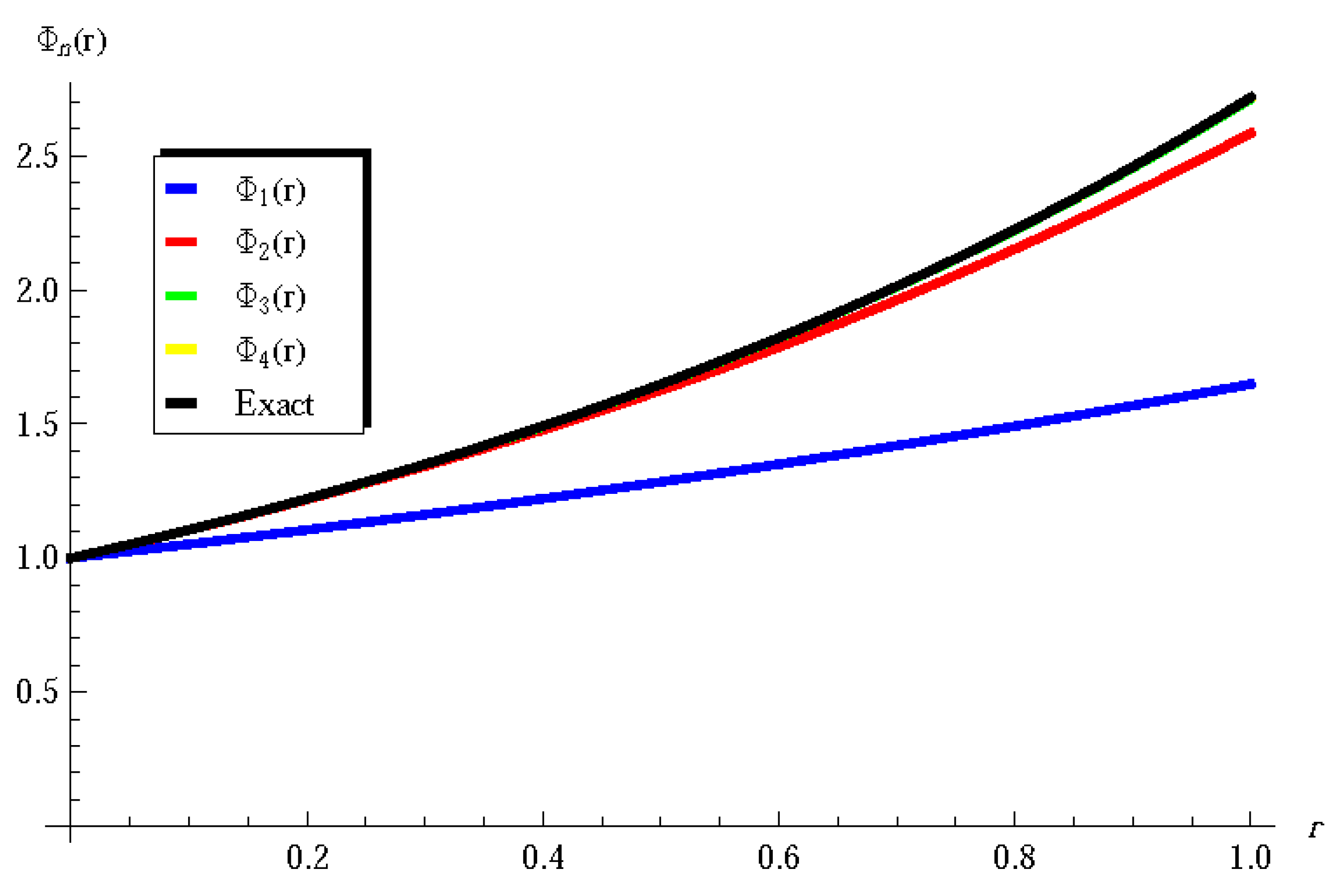
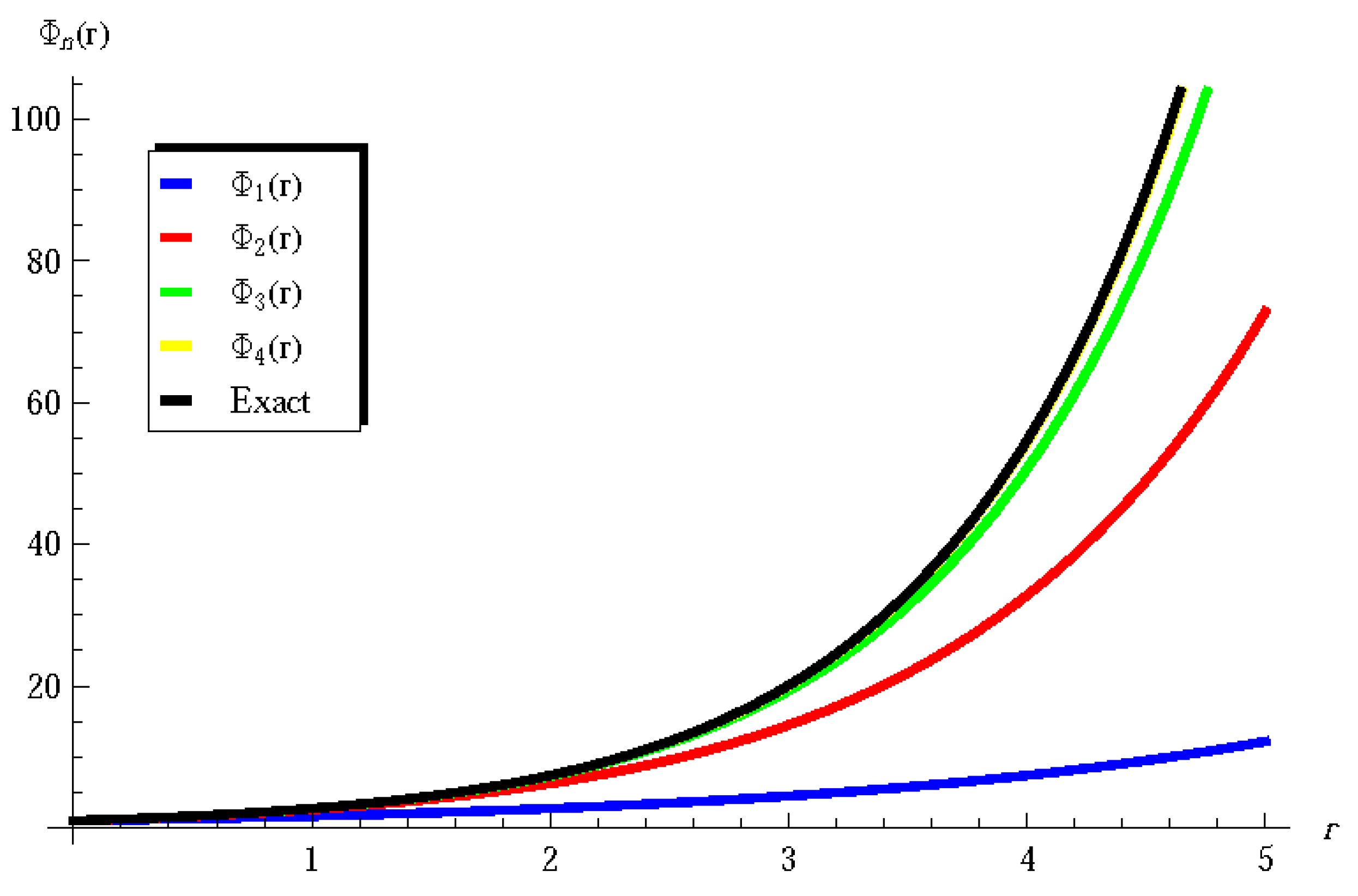
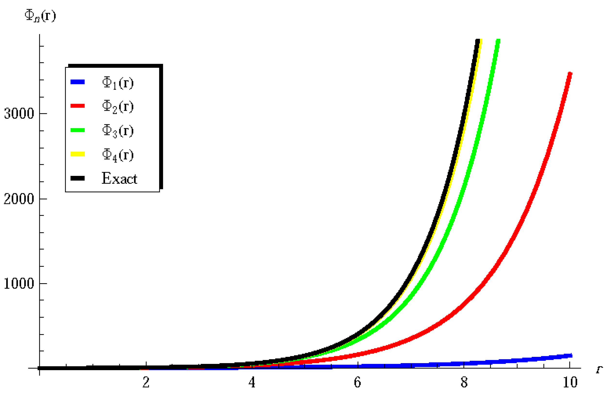
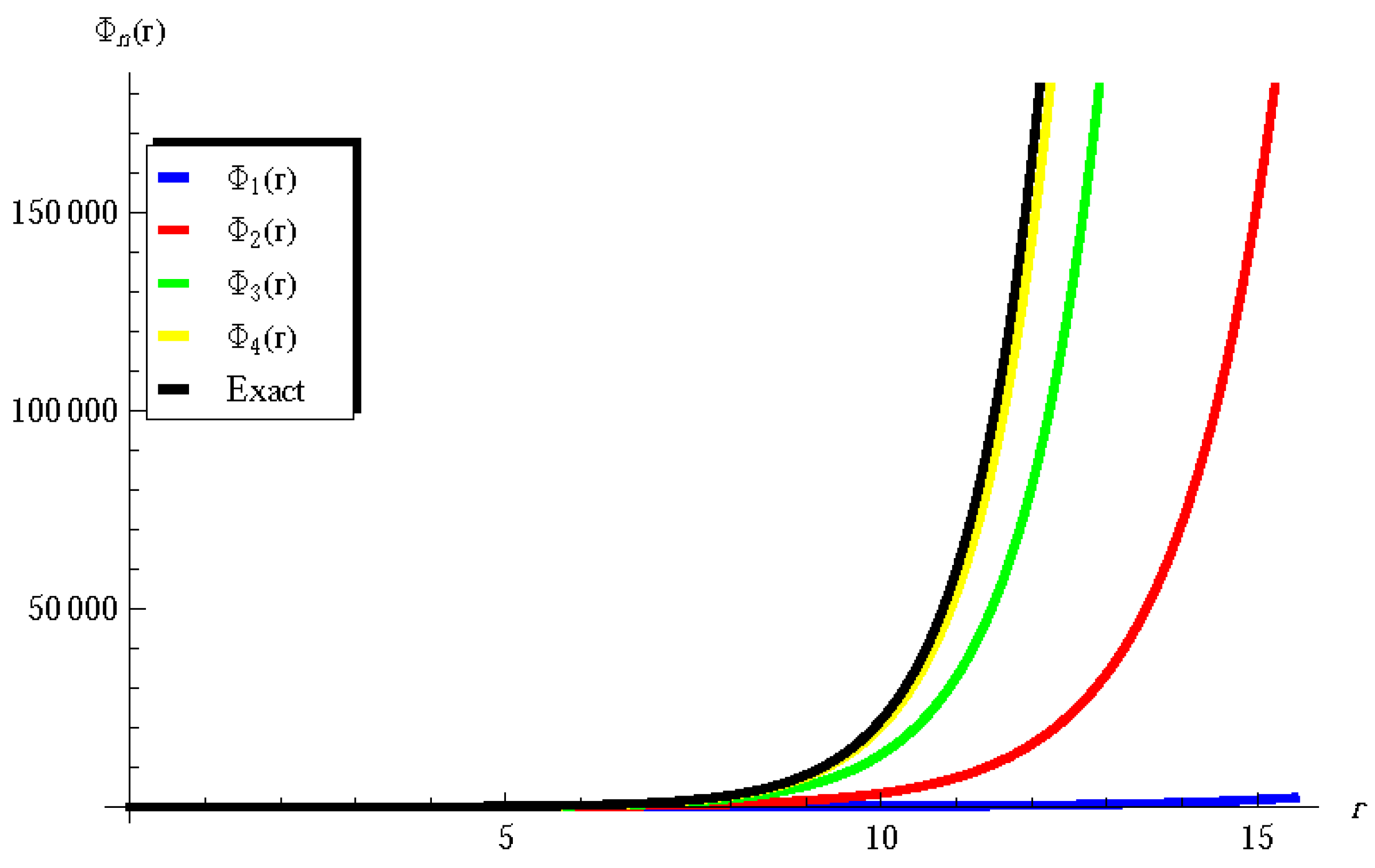
In this context, the approximations using a few terms of the series (45), ${\Phi }_1\left(r\right)$, ${\Phi }_2\left(r\right)$, ${\Phi }_3\left(r\right)$, and ${\Phi }_4\left(r\right)$ are displayed in Figure 1, Figure 2, Figure 3 and Figure 4 at different domains, i.e., at different values of the end point R. These figures show that the convergence of our approximations is verified, even by using a few terms of the series (45). Furthermore, the approximations ${\Phi }_n\left(r\right)$ converge rapidly to the exact solution, especially at $n=3,4$ (Figure 1, $R=1$) and $n=4$ (Figure 2, Figure 3 and Figure 4 when $R=5,10,15$, respectively). It may be concluded from Figure 1, Figure 2, Figure 3 and Figure 4 that the 4-term approximation, i.e., ${\Phi }_4\left(r\right)$ is in full agreement with the exact solution in the following four different domains $0<r\le R$ ($R=1,5,10,15$). In other extended domains $0<r\le R$ ($R>15$), the number of terms n may be increased to achieve the agreement between the current approximations ${\Phi }_n\left(r\right)$ and the exact solution.

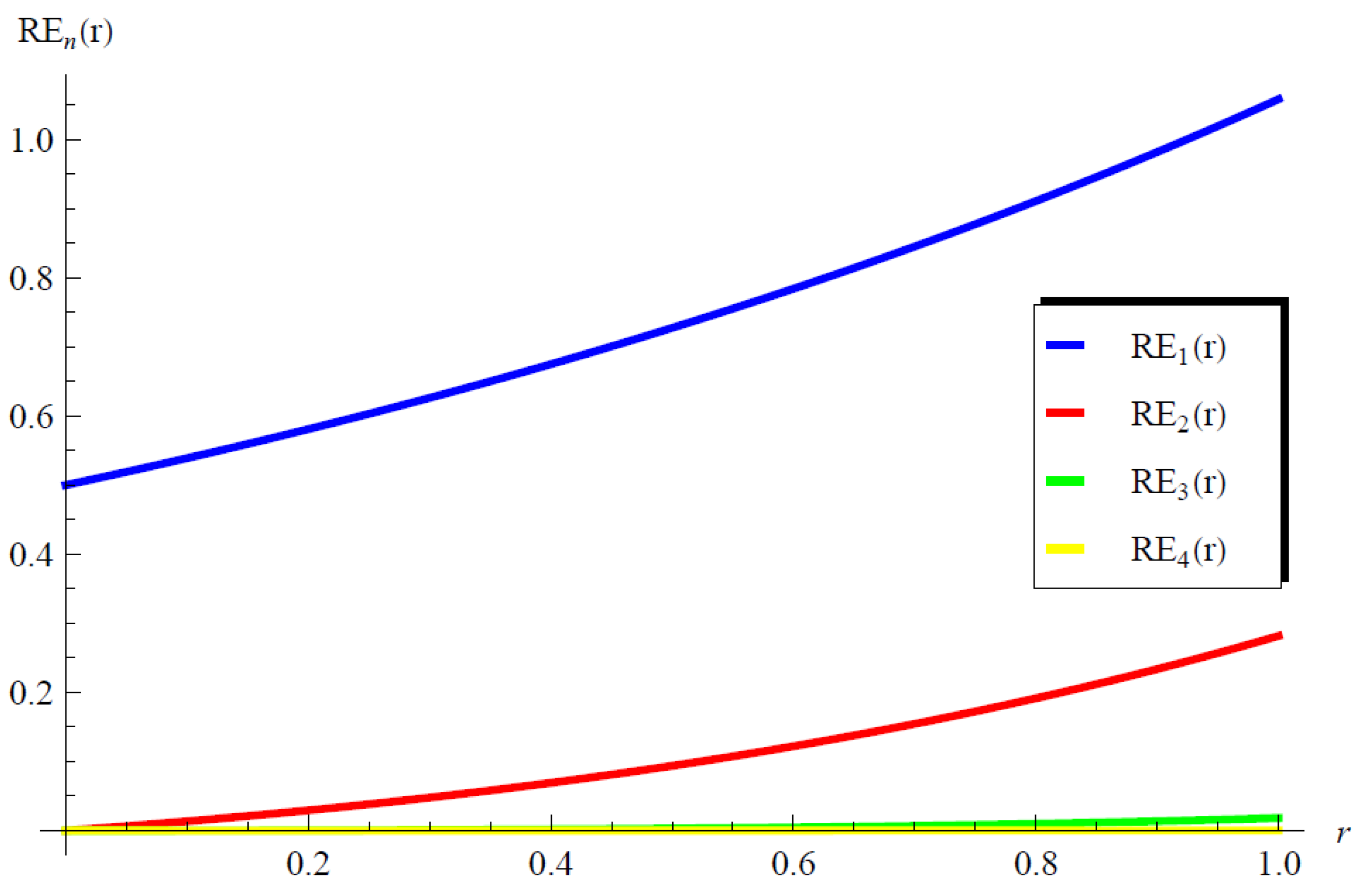
In order to explore the error analysis, numerical calculations are conducted to estimate the residual $R{E}_n\left(r\right)$, defined by [8,31].

$$R{E}_n\left(r\right)=\left|{\Phi }_n^{\prime }\left(r\right)-\frac{1}{2}{\Phi }_n\left(r\right)-\frac{1}{2}{e}^{\frac{r}{2}}{\Phi }_n\left(\frac{r}{2}\right)\right|,n\ge 1.$$

(46)

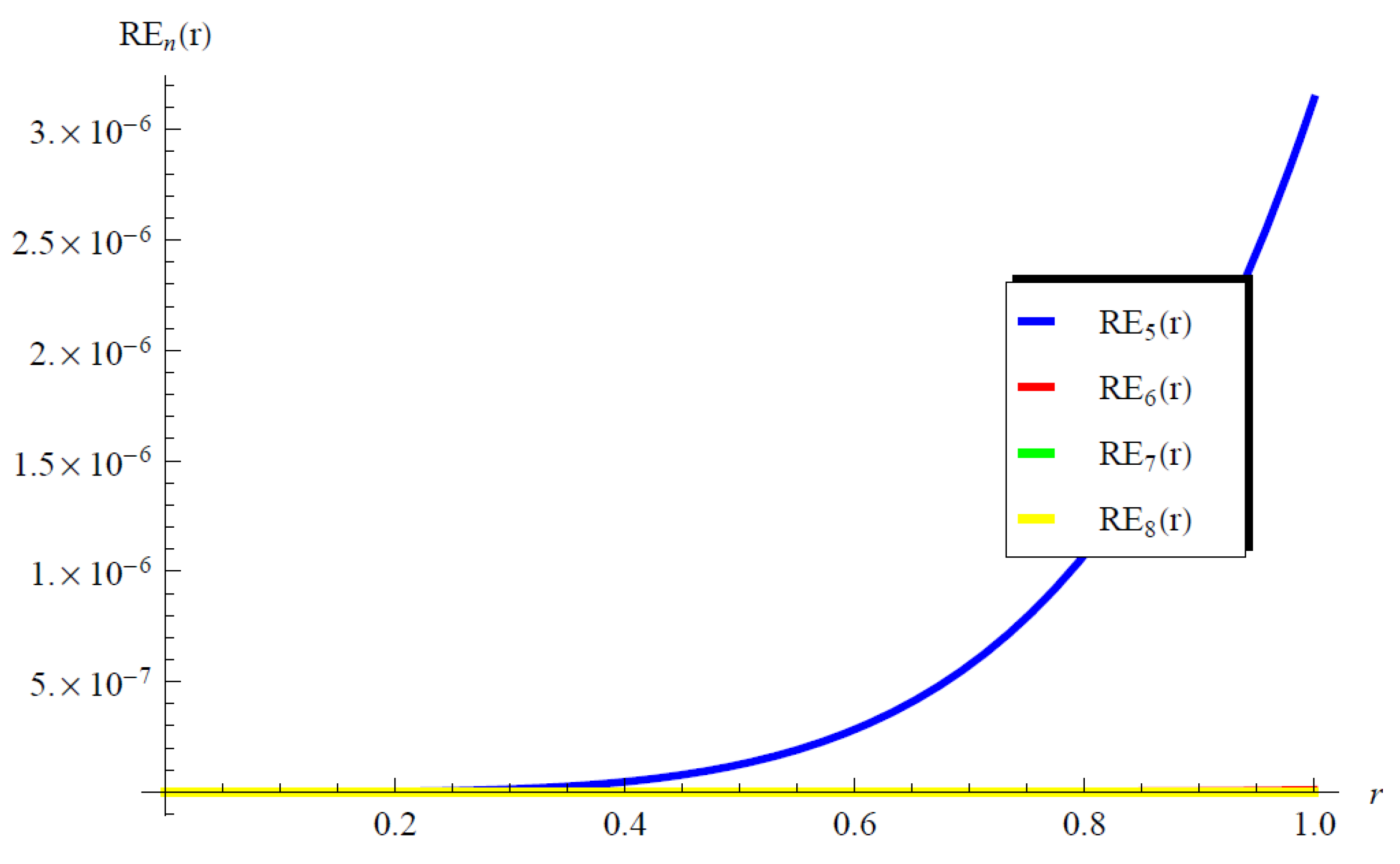
For this purpose, calculations of the residuals $R{E}_n\left(r\right)$ for $n=1,2,3,4$ are extracted and depicted in Figure 5. The results in this figure show that $R{E}_n\left(r\right)$ decreases as the number of terms n increases. In particular, at $n=4$ (the yellow curve) an acceptable residual error is given utilizing only 4 terms of the series (45).

The advantage of the proposed LTADM approach is also clear in Figure 6 in which the residuals $R{E}_n\left(r\right)$ for $n=5,6,7,8$ are calculated and displayed. It can be easily seen in Figure 6 that the obtained residuals are smaller than those obtained in Figure 5. This is simply because the number of terms in Figure 6 is increased. As a final note regarding Figure 6, the residual $R{E}_8\left(r\right)$ (the yellow curve) approaches zero in the domain $0<r\le 1$, i.e., at $R=1$. Usually, one may increase the number of terms as needed to achieve the desired accuracy even if the domain of the problem is enlarged by considering $R>1$. Based on the above results, it may be concluded that the LTADM is an effective tool to deal with the current extended version of the PDDE with a coefficient of exponential order.

6. Conclusions

In this paper, two different approaches were applied to solve the extended pantograph delay equation containing a variable coefficient of exponential order. The exact solution of the present model was obtained by the first approach utilizing the standard Maclaurin series expansion (MSE). The second approach combined the Laplace transform (LT) and the Adomian decomposition method (ADM), known as the LTADM. The LTADM constructed the solution in a closed series form and the accuracy of such a solution was confirmed and verified by conducting several comparisons with the exact solution. To confirm this point, the residual errors were computed, and it was shown that the solution obtained by the LTADM was in full agreement with the exact solution using only a few terms. As further validation, it was indicated that the residual errors tend to zero as the number of terms increases; however, a few terms were sufficient to reach this target. The capability of the present approach to solve other extended versions of the PDDE with variable coefficients may merit further future works. Moreover, exploring the effectiveness of the MSE to deal with nonlinear types of DDEs is essential in the near future.

References

- Sedaghat, S.; Ordokhani, Y.; Dehghan, M. Numerical solution of the delay differential equations of pantograph type via Chebyshev polynomials. Commun. Nonlinear Sci. Numer. Simul. 2012, 17, 4815–4830. [Google Scholar] [CrossRef]
- Tohidi, E.; Bhrawy, A.H.; Erfani, K. A collocation method based on Bernoulli operational matrix for numerical solution of generalized pantograph equation. Appl. Math. Model. 2013, 37, 4283–4294. [Google Scholar] [CrossRef]
- Javadi, S.; Babolian, E.; Taheri, Z. Solving generalized pantograph equations by shifted orthonormal Bernstein polynomials. J. Comput. Appl. Math. 2016, 303, 1–14. [Google Scholar] [CrossRef]
- Shen, J.; Tang, T.; Wang, L. Spectral Methods: Algorithms, Analysis and Applications; Springer: Berlin/Heidelberg, Germany, 2011; Volume 41. [Google Scholar]
- Ezz-Eldien, S.S. On solving systems of multi-pantograph equations via spectral tau method. Appl. Math. Comput. 2018, 321, 63–73. [Google Scholar] [CrossRef]
- Yang, C.; Hou, J.; Lv, X. Jacobi spectral collocation method for solving fractional pantograph delay differential equations. Eng. Comput. 2022, 38, 1985–1994. [Google Scholar] [CrossRef]
- Al-Enazy, A.H.S.; Ebaid, A.; Algehyne, E.A.; Al-Jeaid, H.K. Advanced Study on the Delay Differential Equation y′(t) = ay(t) + by(ct). Mathematics 2022, 10, 4302. [Google Scholar] [CrossRef]
- Albidah, A.B.; Kanaan, N.E.; Ebaid, A.; Al-Jeaid, H.K. Exact and Numerical Analysis of the Pantograph Delay Differential Equation via the Homotopy Perturbation Method. Mathematics 2023, 11, 944. [Google Scholar] [CrossRef]
- Isik, O.R.; Turkoglu, T. A rational approximate solution for generalized pantograph-delay differential equations. Math. Methods Appl. Sci. 2016, 39, 2011–2024. [Google Scholar] [CrossRef]
- Jafari, H.; Mahmoudi, M.; Noori Skandari, M.H. A new numerical method to solve pantograph delay differential equations with convergence analysis. Adv. Differ. Equ. 2021, 2021, 129. [Google Scholar] [CrossRef]
- El-Zahar, E.R.; Ebaid, A. Analytical and Numerical Simulations of a Delay Model: The Pantograph Delay Equation. Axioms 2022, 11, 741. [Google Scholar] [CrossRef]
- Bakodah, H.O.; Ebaid, A. Exact solution of Ambartsumian delay differential equation and comparison with Daftardar-Gejji and Jafari approximate method. Mathematics 2018, 6, 331. [Google Scholar] [CrossRef]
- Dogan, N. Solution of the system of ordinary differential equations by combined Laplace transform-Adomian decomposition method. Math. Comput. Appl. 2012, 17, 203–211. [Google Scholar] [CrossRef]
- Ra, P. Application of Laplace transforms to solve ODE using MATLAB. J. Inform. Math. Sci. 2015, 7, 93–97. [Google Scholar]
- Handibag, S.S.; Karande, B.D. Laplace substitution method for n th-order linear and non-linear PDEs involving mixed partial derivatives. Int. Res. J. Eng. Technol. 2015, 2, 378–388. [Google Scholar]
- Alshikh, A.A.; Mahgob, M.M. A comparative study between Laplace transform and two new integrals “Elzaki” transform and “Aboodh” transform. Pure Appl. Math. J. 2016, 5, 145–150. [Google Scholar] [CrossRef]
- Atangana, A.; Alkaltani, B.S. A novel double integral transform and its applications. J. Nonlinear Sci. Appl. 2016, 9, 424–434. [Google Scholar] [CrossRef]
- Zhou, H.; Yang, L.; Agarwal, P. Solvability for fractional p-Laplacian differential equations with multipoint boundary conditions at resonance on infinite interval. J. Appl. Math. Comput. 2017, 53, 51–76. [Google Scholar] [CrossRef]
- Liang, X.; Gao, F.; Gao, Y.N.; Yang, X.J. Applications of a novel integral transform to partial differential equations. J. Nonlinear Sci. Appl. 2017, 10, 528–534. [Google Scholar] [CrossRef]
- Khaled, S.M. The exact effects of radiation and joule heating on Magnetohydrodynamic Marangoni convection over a flat surface. Therm. Sci. 2018, 22, 63–72. [Google Scholar] [CrossRef]
- Pavani, P.V.; Priya, U.L.; Reddy, B.A. Solving differential equations by using Laplace transforms. Int. J. Res. Anal. Rev. 2018, 5, 1796–1799. [Google Scholar]
- Agarwal, P.; Ntouyas, S.K.; Jain, S.; Chand, M.; Singh, G. Fractional kinetic equations involving generalized k-Bessel function via Sumudu transform. Alex. Eng. J. 2018, 57, 1937–1942. [Google Scholar] [CrossRef]
- Restrepo, J.E.; Piedrahita, A.; Agarwal, P. Multidimensional Fourier transform and fractional derivative. Proc. Jangjeon Math. Soc. 2019, 22, 269–277. [Google Scholar]
- Faraj, B.M.; Ahmed, F.W. On the MATLAB technique by using Laplace transform for solving second order ODE with initial conditions exactly. Matrix Sci. Math. 2019, 3, 8–10. [Google Scholar] [CrossRef]
- Mousa, A.; Elzaki, M. Solution of volterra integro-differential equations by triple Laplace transform. Irish Interdiscip. J. Sci. Res. 2019, 3, 67–72. [Google Scholar]
- Dhunde, R.R.; Waghmare, G.L. Double Laplace iterative method for solving nonlinear partial differential equations. New Trends Math. Sci. 2019, 7, 138–149. [Google Scholar] [CrossRef]
- Ziane, D.; Cherif, M.H.; Cattani, C.; Belghaba, K. Yang-Laplace decomposition method for nonlinear system of local fractional partial differential equations. Appl. Math. Nonlinear Sci. 2019, 4, 489–502. [Google Scholar] [CrossRef]
- Mastoi, S.; Othman, W.A.; Nallasamy, K. Randomly generated grids and Laplace Transform for partial differential equations. Int. J. Disaster Recovery Bus. Contin. 2020, 11, 1694–1702. [Google Scholar]
- Ebaid, A.; Alharbi, W.; Aljoufi, M.D.; El–Zahar, E.R. The exact solution of the falling body problem in three–dimensions: Comparative study. Mathematics 2020, 8, 1726. [Google Scholar] [CrossRef]
- Spiegel, M.R. Spiegel, Laplace Transforms; McGraw-Hill. Inc.: New York, NY, USA, 1965. [Google Scholar]
- Alrebdi, R.; Al-Jeaid, H.K. Accurate Solution for the Pantograph Delay Differential Equation via Laplace Transform. Mathematics 2023, 11, 2031. [Google Scholar] [CrossRef]
- Srinivasa, K.; Mundewadi, R.A. Wavelets approach for the solution of nonlinear variable delay differential equations. Int. J. Math. Comput. Eng. 2023, 1, 139–148. [Google Scholar] [CrossRef]
Figure 1.
Comparison between the approximations for and the exact solution in the domain (i.e., ).
Figure 2.
Figure 3.
Figure 4.
Figure 5.
The residual for in the domain (i.e., ).
Figure 6.
Disclaimer/Publisher’s Note: The statements, opinions and data contained in all publications are solely those of the individual author(s) and contributor(s) and not of MDPI and/or the editor(s). MDPI and/or the editor(s) disclaim responsibility for any injury to people or property resulting from any ideas, methods, instructions or products referred to in the content. |
© 2024 by the authors. Licensee MDPI, Basel, Switzerland. This article is an open access article distributed under the terms and conditions of the Creative Commons Attribution (CC BY) license (https://creativecommons.org/licenses/by/4.0/).
Share and Cite
MDPI and ACS Style
Alrebdi, R.; Al-Jeaid, H.K. Two Different Analytical Approaches for Solving the Pantograph Delay Equation with Variable Coefficient of Exponential Order. Axioms 2024, 13, 229. https://0-doi-org.brum.beds.ac.uk/10.3390/axioms13040229
AMA Style
Alrebdi R, Al-Jeaid HK. Two Different Analytical Approaches for Solving the Pantograph Delay Equation with Variable Coefficient of Exponential Order. Axioms. 2024; 13(4):229. https://0-doi-org.brum.beds.ac.uk/10.3390/axioms13040229
Chicago/Turabian StyleAlrebdi, Reem, and Hind K. Al-Jeaid. 2024. "Two Different Analytical Approaches for Solving the Pantograph Delay Equation with Variable Coefficient of Exponential Order" Axioms 13, no. 4: 229. https://0-doi-org.brum.beds.ac.uk/10.3390/axioms13040229
Note that from the first issue of 2016, this journal uses article numbers instead of page numbers. See further details here.