Projector Approach to Constructing Asymptotic Solution of Initial Value Problems for Singularly Perturbed Systems in Critical Case


1
Voronezh State University, Voronezh 394018, Russia
2
Voronezh Institute of Law and Economics, Voronezh 394042, Russia
3
Federal Research Center “Computer Science and Control” of Russian Academy of Sciences, Moscow 119333, Russia
†
Voronezh State University, Universitetskaya pl.,1, Voronezh 394018, Russia.
Axioms 2019, 8(2), 56; https://0-doi-org.brum.beds.ac.uk/10.3390/axioms8020056
Submission received: 13 February 2019
/
Revised: 20 April 2019
/
Accepted: 21 April 2019
/
Published: 8 May 2019
(This article belongs to the Special Issue Singularly Perturbed Problems: Asymptotic Analysis and Approximate Solution)
Abstract
:Under some conditions, an asymptotic solution containing boundary functions was constructed in a paper by Vasil’eva and Butuzov (Differ. Uravn. 1970, 6(4), 650–664 (in Russian); English transl.: Differential Equations 1971, 6, 499–510) for an initial value problem for weakly non-linear differential equations with a small parameter standing before the derivative, in the case of a singular matrix standing in front of the unknown function. In the present paper, the orthogonal projectors onto and (the prime denotes the transposition) are used for asymptotics construction. This approach essentially simplifies understanding of the algorithm of asymptotics construction.
1. Introduction
The bibliography of publications devoted to singularly perturbed problems is very extensive. Most of them deal with problems in which a degenerate equation, following from the original one where a small parameter is equal to zero, is resolvable with respect to a fast component of an unknown variable. If it is not so, then this more complicated case is known as critical [1], singular [2], nonstandard [3], or as a case where the unperturbed (degenerate) system is situated on the spectrum [4]. Numerous applications of singularly perturbed systems in the critical cases have been listed in [5].
Vasil’eva and Butuzov were the first to study initial value problems for singularly perturbed differential and difference systems in the critical case. Asymptotic solutions of boundary value problems for such systems have been obtained in [1,2,6]. Numerical methods for singularly perturbed systems in the critical case have been researched in [7] for initial value problems, and in [8] for boundary value problems.
An asymptotic solution containing boundary functions for the initial value problem of the weakly non-linear differential equation in a real m-dimensional space X:
where and the matrix is singular, has been constructed in [4]. A discrete analogue of problem (1)-(2) was also considered. The results from this paper are also presented in [1,9]. In these publications, the purpose of studying equations of the last form is also explained. Here and further means a small parameter, and the matrix and the m-dimensional vector-function are sufficiently smooth with respect to their arguments.
In contrast [4], the projector approach will be used in this paper for constructing an asymptotic solution of problem (1)-(2). It allows us to represent the algorithm of the boundary functions method for constructing an asymptotic solution of initial-value singularly perturbed problems in the critical case more clearly than in [4].
Note that the projector approach has been used in [10] for constructing the zero-order asymptotic solution for a singularly perturbed linear-quadratic control problem in the critical case.
We will assume the same assumptions as in [4] that the matrix has for each m eigenvalues , and that they satisfy the conditions:
Assumption 1.
for , .
Assumption 2.
All k eigenvectors of the matrix , corresponding to , , are linearly independent.
Following [4], we will here use eigenvectors having the same smoothness as the matrix . The existence of such eigenvectors has been proved in [11].
Furthermore, some assumptions will be yet added.
The transposition will be denoted by the prime. By I, as usual, we mean the identity operator. For the expansion of a function into the series with respect to integer non-negative powers of , we introduce the notation .
The paper is organized as follows. In Section 2, we present the standard decomposition of the original system (1) into systems with respect to functions from the asymptotic solution, depending on t, and with respect to so-called boundary functions, depending on the argument . In the next section, we introduce orthogonal projectors of the space X onto and . Based on these projectors, the algorithm of constructing the zero-order asymptotic approximation of a solution of problem (1)-(2) is given in Section 4, and the algorithm of constructing the n-th order asymptotic approximation, , is developed in Section 5. Table 1 and Table 2 in these two sections show the sequence of actions for finding asymptotics terms. In the sixth section, we present an example illustrating the projector approach for constructing the first-order asymptotic approximation. The last section presents our conclusions.
2. Problem Decomposition
In view of [4], we will seek the asymptotic solution of problem (1)-(2) in the form:
where , , . Functions will be found as in [4] with the help of the additional condition
Following tradition (see, for instance, [1], p. 8), a series with terms depending on the original argument t is called regular series, in contrast with boundary series consisting of so-called boundary functions depending on the argument , which are essential only for arguments in some vicinities of points where additional conditions are prescribed (in a vicinity of zero in the considered case).
As usual in the theory of singular perturbations, the following representation will be used
where and
Substituting expansion (3) into (1) and equating terms of the same order of separately depending on t and , we obtain the following equations for the terms of series (3):
where ,
3. Space Decomposition
Further, we will use the decompositions of the space X in the orthogonal sums (see, for instance, [12], p. 38)
Orthogonal projectors and of the space X onto the subspaces and , respectively, corresponding to the decompositions of the space X into two last orthogonal sums, will be applied. We can write the explicit form of these projectors. Namely, let and , where are the eigenvectors of the matrix corresponding to eigenvalues , . Following [9], we believe that the eigenvectors have been chosen in such a way that is the identity matrix. We explain that this is possible. The invertibility of the matrix is proved in [1]. If , then we take the columns of the matrix as .
It easily follows from Assumption 2 that the matrices and are invertible. It is not difficult to see that and are orthogonal projectors of the space X onto the subspaces and , respectively, corresponding to the decompositions of the space X into the orthogonal sums.
The operator
has the inverse operator. It will be denoted as .
The following condition is assumed.
Assumption 3.
For each the operator is stable—that is, all eigenvalues of this operator have negative real parts.
It is not difficult to prove that the operator is invertible. Let us take a vector x from . Then, , where and , are some scalar functions. Consider the equation . It follows from this that . Since is a identity matrix, then , which gives the provable invertibility.
4. Zero-Order Asymptotic Solution
From (5), we have the equation for :
Hence,
From (6), we have the equation for
This equation is equivalent to two ones:
In view of Assumption 3, we obtain a unique solution of initial problem (10)-(11) satisfying the inequality
with some positive constants c and independent of (see, for instance, [13], p. 106). In this estimate, any norm may be used, since all norms in a finite dimensional space are equivalent. Functions satisfying the last inequality are called exponential-type boundary functions.
From (12), we get the equality . Since as , then . Using the exponential estimate for , we uniquely define the exponential-type boundary function , namely,
Hence, the exponential-type boundary function has been found. Then, we can get the initial value from (7):
In view of (5), the equation for has the form
Taking into account (9), we can write the solvability condition for the last equation in the form
Since
we obtain the equation
If operator is constant, then projectors and are constant too, and the last equation has the form
We will yet assume the condition.
A similar assumption regarding the solvability of some initial-value problem for a non-linear equation of the smaller dimension than the original one was presented in [1] (Assumption IV, p. 13).
Thus, the function is defined. Hence, the zero-order asymptotics for a solution of problem (1)-(2) is found.
The following Table 1 shows the sequence of finding zero-order asymptotics terms.
5. Higher-Order Asymptotic Solutions
Suppose that the terms and of expansion (3), , have been found.
From equation (5) with , we obtain the relation
where the right-hand side is known. Applying the operator to this equation, we have
From here, we find:
Then, we can find from (8) with the initial value
The equation (6) with has the form
This equation is equivalent to two ones.
The sum of two last summands in the right-hand side in (20) is a known exponential-type boundary function. Therefore, in view of Assumption 3, we can find from (19) and (20) the exponential-type boundary function . Note that the proof of exponential estimates for boundary functions is given in detail in monograph [14].
As the function in the braces on the right-hand side in (21) is a known exponential type boundary function, we can get from (21) the exponential-type boundary function , namely
Hence, the exponential-type boundary function is defined. Then, we can find from (8) with the initial value
Writing out equation (5) with , we get
The solvability condition for this equation has the form
In view of (15), we obtain from here the equation
If operator is constant, then this equation has the form:
It should be noted that equation (24) is linear with respect to . As has been found (see (18)), we can define the function from (23) and (24).
Hence, we have found the terms of the n-th order in expansion (3).
The previous arguments have, as a consequence, the following assertion.
6. Illustrative Example
Here, , ; , ; ,
Hence,
We will construct the first-order approximation for the asymptotic solution of problem (26)-(27) using projectors P and Q.
Relation (9), in this case, has the form:
Therefore, .
From (10), we get .
Equation (11) has the form:
Taking into account the initial value found from (10), we obtain from the last equation
From (13), we find
In view of the last two relations, we have .
Thus, we have found the zero-order asymptotic solution of form (3) for the solution of problems (26)-(27). Namely, we have
Now, we will seek for the first-order asymptotics.
Equation (18) for has the form:
Therefore, .
From (19) with , we get .
Equation (20) for has the form:
From the last two relations, we obtain .
From (22) with , we find
In view of the last two relations, we have
Thus, we have found for problems (26)-(27) the first-order asymptotic solution of form (3) . Namely, we have
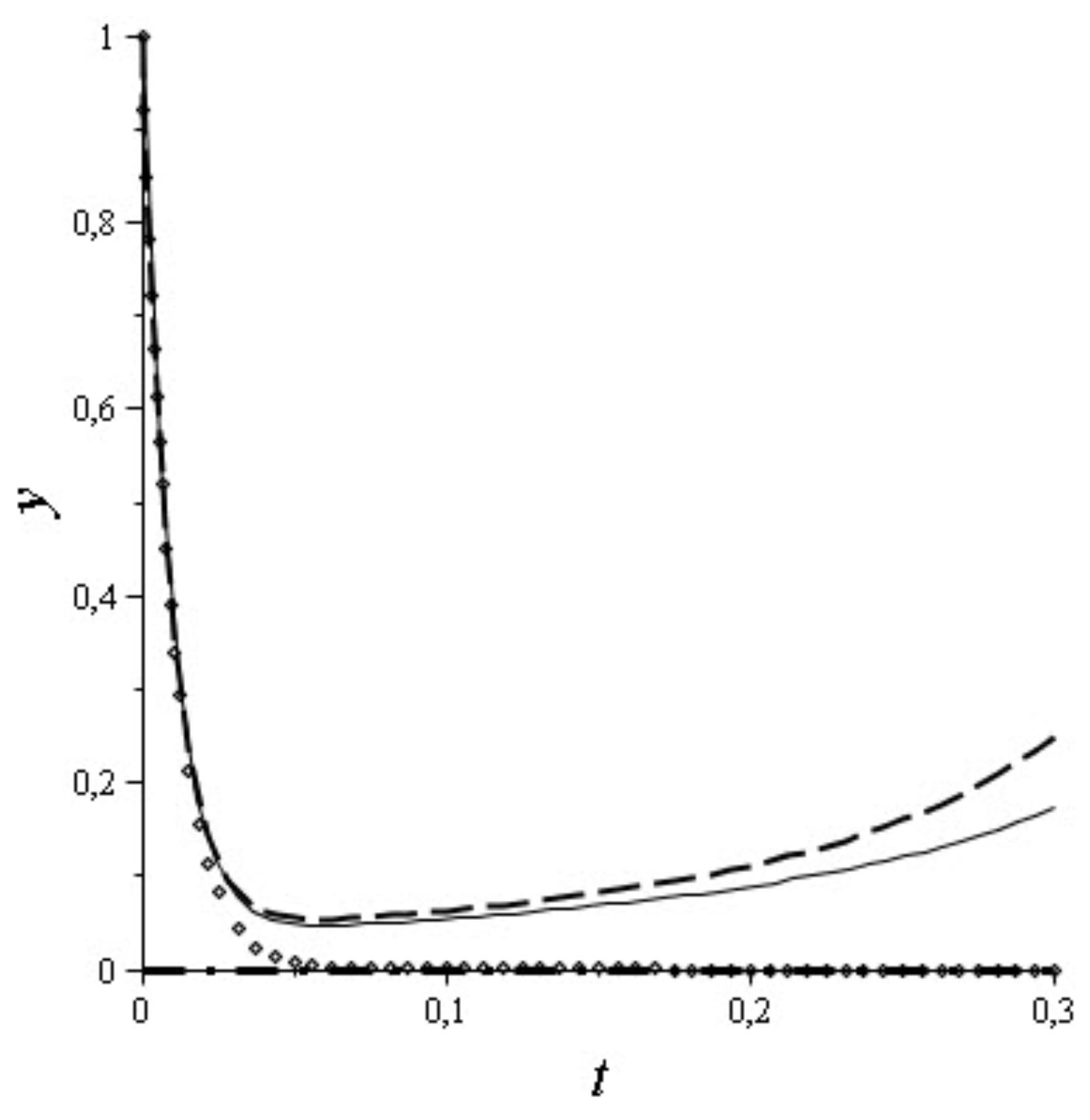
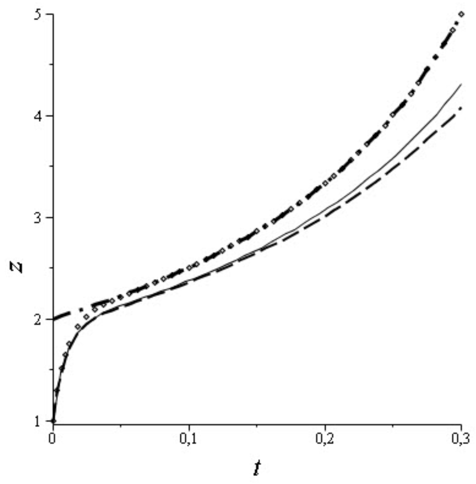
Of course, these results can be obtained using the algorithm from [4], but we would like to demonstrate here the use of projectors for finding asymptotics terms. The results obtained by Maple 13 are given in Figure 1 and Figure 2. They have been presented for the completeness of the paper. The solid line represents the exact solution; the dash-dotted line—the solution of the degenerate problem, the line consisting of squares represents the zero-order approximation; and the dash line represents the the first-order approximation. These graphs show that an asymptotic solution is closer to the exact one if we use higher-order asymptotics. If we use the smaller value of , then it will result in an asymptotic solution more similar to the exact one. The graphs of the solution of the degenerate problem and the zero-order approximation illustrate the known property of boundary functions that are essential only for arguments in some vicinities of points where additional conditions are prescribed.
7. Conclusions
This paper dealt with a new approach to the algorithm of the method of boundary functions from [4] for asymptotic solving initial value problem of form (1)-(2) in the critical case. Namely, the algorithm was formulated with the help of orthogonal projectors of the space X onto and . Such an approach clearly shows the structure of the algorithm for finding asymptotics terms, given in Table 1 and Table 2 of the paper.
Funding
This research was funded by the RUSSIAN SCIENCE FOUNDATION, grant number 17-11-01220.
Acknowledgments
The author thank the anonymous referees for carefully reading the paper and for the numerous critical and constructive comments that have helped to improve the paper text. She thanks also N. T. Hoai for useful discussions and M. A. Kalashnikova for the help in printing the paper text.
Conflicts of Interest
The author declare no conflict of interest. The funders had no role in the design of the study; in the collection, analyses, or interpretation of data; in the writing of the manuscript, or in the decision to publish the results.
References
- Vasil’eva, A.B.; Butuzov, V.F. Singularly Perturbed Equations in Critical Cases; Moscow University: Moscow, Russia, 1978; 107p, English transl.: University ofWisconsin-Madison: Wisconsin, WI, USA, 1980; 165p. [Google Scholar]
- O’Malley, R.E., Jr. A singular singularly-perturbed linear boundary value problem. SIAM J. Math. Anal. 1979, 10, 695–708. [Google Scholar] [CrossRef]
- Khalil, H.K. Feedback control of nonstandard singularly perturbed systems. IEEE Trans. Autom. Control 1989, 34, 1052–1060. [Google Scholar] [CrossRef]
- Butuzov, V.F.; Vasil’eva, A.B. Differential and difference systems of equations with a small parameter in the case when the unperturbed (degenerate) system is situated on the spectrum. Differ. Uravn. 1971, 6, 650–664. (In Russian); English transl.: Differ. Equ. 1971, 6, 499–510. [Google Scholar]
- Gu, Z.M.; Nefedov, N.N.; O’Malley, R.E., Jr. On singular singularly perturbed initial value problems. SIAM J. Appl. Math. 1989, 49, 1–25. [Google Scholar] [CrossRef]
- Schmeiser, C.; Wess, R. Asymptotic analysis of singular singularly perturbed boundary value problems. SIAM J. Math. Anal. 1986, 17, 560–579. [Google Scholar] [CrossRef]
- O’Malley, R.E., Jr.; Flaherty, J.E. Analytical and numerical methods for nonlinear singular singularly-perturbed initial value problems. SIAM J. Appl. Math. 1980, 38, 225–248. [Google Scholar] [CrossRef]
- Ascher, U. On some difference schemes for singular singularly-perturbed boundary value problems. Numer. Math. 1985, 46, 1–30. [Google Scholar] [CrossRef]
- Vasil’eva, A.B.; Butuzov, V.F.; Kalachev, L.V. The Boundary Function Method for Singular Perturbation Problems; SIAM: Philadelphia, PA, USA, 1995. [Google Scholar]
- Kurina, G.A.; Hoai, N.T. Projector approach for constructing the zero order asymptotic solution for the singularly perturbed linear-quadratic control problem in a critical case. AIP Conf. Proc. 2018, 1997, 020073-1–020073-7. [Google Scholar] [CrossRef]
- Sibuya, Y. Some global properties of matrices of functions of one variable. Math. Ann. 1965, 161, 67–77. [Google Scholar] [CrossRef]
- Kato, T. Perturbation Theory for Linear Operators; Mir: Moscow, Russia, 1972; 740p. [Google Scholar]
- Daletskii, Y.L.; Krein, M.G. Stability of Solutions of Differential Equations in Banach Space; Nauka: Moscow, Russia, 1970; 536p. [Google Scholar]
- Vasil’eva, A.B.; Butuzov, V.F. Asymptotic Expansions of Solutions of Singularly Perturbed Equations; Nauka: Moscow, Russia, 1973; 272p. [Google Scholar]
Figure 1.
Trajectory with and its approximations.

Figure 2.
Trajectory with and its approximations.


© 2019 by the author. Licensee MDPI, Basel, Switzerland. This article is an open access article distributed under the terms and conditions of the Creative Commons Attribution (CC BY) license (http://creativecommons.org/licenses/by/4.0/).
Share and Cite
MDPI and ACS Style
Kurina, G. Projector Approach to Constructing Asymptotic Solution of Initial Value Problems for Singularly Perturbed Systems in Critical Case. Axioms 2019, 8, 56. https://0-doi-org.brum.beds.ac.uk/10.3390/axioms8020056
AMA Style
Kurina G. Projector Approach to Constructing Asymptotic Solution of Initial Value Problems for Singularly Perturbed Systems in Critical Case. Axioms. 2019; 8(2):56. https://0-doi-org.brum.beds.ac.uk/10.3390/axioms8020056
Chicago/Turabian StyleKurina, Galina. 2019. "Projector Approach to Constructing Asymptotic Solution of Initial Value Problems for Singularly Perturbed Systems in Critical Case" Axioms 8, no. 2: 56. https://0-doi-org.brum.beds.ac.uk/10.3390/axioms8020056
Note that from the first issue of 2016, this journal uses article numbers instead of page numbers. See further details here.