Distributed-Order Non-Local Optimal Control


Center for Research and Development in Mathematics and Applications (CIDMA), Department of Mathematics, University of Aveiro, 3810-193 Aveiro, Portugal
*
Author to whom correspondence should be addressed.
†
This research is part of first author’s Ph.D. project, which is carried out at the University of Aveiro under the Doctoral Program in Applied Mathematics of Universities of Minho, Aveiro, and Porto (MAP-PDMA).
‡
These authors contributed equally to this work.
Axioms 2020, 9(4), 124; https://0-doi-org.brum.beds.ac.uk/10.3390/axioms9040124
Submission received: 9 September 2020
/
Revised: 16 October 2020
/
Accepted: 22 October 2020
/
Published: 25 October 2020
(This article belongs to the Special Issue Nonlinear Differential Equations and Dynamical Systems: Theory and Applications)
Abstract
:Distributed-order fractional non-local operators were introduced and studied by Caputo at the end of the 20th century. They generalize fractional order derivatives/integrals in the sense that such operators are defined by a weighted integral of different orders of differentiation over a certain range. The subject of distributed-order non-local derivatives is currently under strong development due to its applications in modeling some complex real world phenomena. Fractional optimal control theory deals with the optimization of a performance index functional, subject to a fractional control system. One of the most important results in classical and fractional optimal control is the Pontryagin Maximum Principle, which gives a necessary optimality condition that every solution to the optimization problem must verify. In our work, we extend the fractional optimal control theory by considering dynamical system constraints depending on distributed-order fractional derivatives. Precisely, we prove a weak version of Pontryagin’s maximum principle and a sufficient optimality condition under appropriate convexity assumptions.
Keywords:
distributed-order fractional calculus; basic optimal control problem; Pontryagin extremalsMSC:
26A33; 49K151. Introduction
Distributed-order fractional operators were introduced and studied by Caputo at the end of the previous century [1,2]. They can be seen as a kind of generalization of fractional order derivatives/integrals in the sense that these operators are defined by a weighted integral of different orders of differentiation over a certain range. This subject gained more interest at the beginning of the current century by researchers from different mathematical disciplines, through attempts to solve differential equations with distributed-order derivatives [3,4,5,6]. Moreover, at the same time, in the domain of applied mathematics, those distributed-order fractional operators have started to be used, in a satisfactory way, to describe some complex phenomena modeling real world problems—see, for instance, works in viscoelasticity [7,8] and in diffusion [9]. Today, the study of distributed-order systems with fractional derivatives is a hot subject—see, e.g., [10,11,12] and references therein.
Fractional optimal control deals with optimization problems involving fractional differential equations, as well as a performance index functional. One of the most important results is the Pontryagin Maximum Principle, which gives a first-order necessary optimality condition that every solution to the dynamic optimization problem must verify. By applying such a result, it is possible to find and identify candidate solutions to the optimal control problem. For the state of the art on fractional optimal control, we refer the readers to [13,14,15] and references therein. Recently, distributed-order fractional problems of the calculus of variations were introduced and investigated in [16]. Here, our main aim is to extend the distributed-order fractional Euler–Lagrange equation of [16] to the Pontryagin setting (see Remark 2).
Regarding optimal control for problems with distributed-order fractional operators, the results are rare and reduce to the following two papers: [17,18]. Both works develop numerical methods while, in contrast, here we are interested in analytical results (not in numerical approaches). Moreover, our results are new and bring new insights. Indeed, in [17], the problem is considered with Riemann–Liouville distributed derivatives, while in our case we consider optimal control problems with Caputo distributed derivatives. We must also note an inconsistency in [17]: when one defines the control system with a Riemann–Liouville derivative, then in the adjoint system it should appear as a Caputo derivative—when one considers optimal control problems with a control system with Caputo derivatives, the adjoint equation should involve a Riemann–Liouville operator—as a consequence of integration by parts (cf. Lemma 1). This inconsistency has been corrected in [18], where optimal control problems with Caputo distributed derivatives (as in this paper) are considered. Unfortunately, there is still an inconsistency in the necessary optimality conditions of both [17,18]: the transversality conditions are written there exactly as in the classical case, with the multiplier vanishing at the end of the interval, while the correct condition, as we prove in our Theorem 1, should involve a distributed integral operator—see condition (3).
The text is organized as follows. We begin by recalling definitions and necessary results of the literature in Section 2 of preliminaries. Our original results are then given in Section 3. More precisely, we consider fractional optimal control problems where the dynamical system constraints depend on distributed-order fractional derivatives. We prove a weak version of Pontryagin’s maximum principle for the considered distributed-order fractional problems (see Theorem 1) and investigate a Mangasarian-type sufficient optimality condition (see Theorem 2). An example, illustrating the usefulness of the obtained results, is given (see Examples 1 and 2). We end with Section 4 of conclusions, mentioning also some possibilities of future research.
2. Preliminaries
In this section, we recall necessary results and fix notations. We assume the reader to be familiar with the standard Riemann–Liouville and Caputo fractional calculi [19,20].
Let be a real number in and let be a non-negative continuous function defined on such that
This function will act as a distribution of the order of differentiation.
Definition 1
(See [1]). The left and right-sided Riemann–Liouville distributed-order fractional derivatives of a function are defined, respectively, by
where and are, respectively, the left and right-sided Riemann–Liouville fractional derivatives of order α.
Definition 2
(See [1]). The left and right-sided Caputo distributed-order fractional derivatives of a function are defined, respectively, by
where and are, respectively, the left and right-sided Caputo fractional derivatives of order α.
As noted in [16], there is a relation between the Riemann–Liouville and the Caputo distributed-order fractional derivatives:
and
Along the text, we use the notation
where represents the right Riemann–Liouville fractional integral of order .
The next result has an essential role in the proofs of our main results; that is, in the proofs of Theorems 1 and 2.
Lemma 1
(Integration by parts formula [16]). Let x be a continuous function and y a continuously differentiable function. Then,
Next, we recall the standard notion of concave function, which will be used in Section 3.3.
Definition 3
Lemma 2
(See [21]). Let be a continuously differentiable function. Then h is a concave function if and only if it satisfies the so called gradient inequality:
for all .
Finally, we recall a fractional version of Gronwall’s inequality, which will be useful to prove the continuity of solutions in Section 3.1.
Lemma 3
(See [22]). Let α be a positive real number and let , , and be non-negative continuous functions on with monotonic increasing on . If
then
for all .
3. Main Results
The basic problem of optimal control we consider in this work, denoted by (BP), consists in finding a piecewise continuous control and the corresponding piecewise smooth state trajectory solution of the distributed-order non-local variational problem
where functions L and f, both defined on , are assumed to be continuously differentiable in all their three arguments: , . Our main contribution is to prove necessary (Section 3.2) and sufficient (Section 3.3) optimality conditions.
3.1. Sensitivity Analysis
Before we can prove necessary optimality conditions to problem (BP), we need to establish continuity and differentiability results on the state solutions for any control perturbation (Lemmas 4 and 5), which are then used in Section 3.2. The proof of Lemma 4 makes use of the following mean value theorem for integration, that can be found in any textbook of calculus (see Lemma 1 of [23]): if is a continuous function and is an integrable function that does not change the sign on the interval, then there exists a number , such that
Lemma 4
(Continuity of solutions). Let be a control perturbation around the optimal control , that is, for all , , where is a variation and . Denote by its corresponding state trajectory, solution of
Then, we have that converges to the optimal state trajectory when ϵ tends to zero.
Proof.
Starting from the definition, we have, for all , that
Then, by linearity,
and it follows, by definition of the distributed operator, that
Now, using the mean value theorem for integration, and denoting , we obtain that there exists an such that
Clearly, one has
which leads to
Moreover, because f is Lipschitz-continuous, we have
By setting , it follows that
for all . Now, by applying Lemma 3 (the fractional Gronwall inequality), it follows that
The series in the last inequality is a Mittag–Leffler function and thus convergent. Hence, by taking the limit when tends to zero, we obtain the desired result: for all . □
Lemma 5
(Differentiation of the perturbed trajectory). There exists a function η defined on such that
Proof.
Since , we have that
Observe that and when and, by Lemma 4, we have when . Thus, the residue term can be expressed in terms of only, that is, the residue is . Therefore, we have
which leads to
meaning that
We want to prove the existence of the limit , that is, to prove that . This is indeed the case, since is solution of the distributed order fractional differential equation
The intended result is proven. □
3.2. Pontryagin’s Maximum Principle of Distributed-Order
The following result is a necessary condition of Pontryagin type [24] for the basic distributed-order non-local optimal control problem (BP).
Theorem 1
(Pontryagin Maximum Principle for (BP)). If is an optimal pair for (BP), then there exists , called the adjoint function variable, such that the following conditions hold for all t in the interval :
- The optimality condition
- The adjoint equation
- The transversality condition
Proof.
Let be the solution to problem (BP), be a variation, and a real constant. Define , so that . Let be the state corresponding to the control , that is, the state solution of
Note that for all whenever . Furthermore,
Something similar is also true for . Because , it follows from Lemma 4 that, for each fixed t, as . Moreover, by Lemma 5, the derivative exists for each t. The objective functional at is
Next, we introduce the adjoint function . Let be in , to be determined. By the integration by parts formula (see Lemma 1),
and one has
Since the process is assumed to be a maximizer of problem (BP), the derivative of with respect to must vanish at ; that is,
where the partial derivatives of L and f, with respect to x and u, are evaluated at . Rearranging the term and using (5), we obtain that
Setting , it follows that
where the partial derivatives of H are evaluated at . Now, choosing
that is, given the adjoint equation (2) and the transversality condition (3), it yields
and, by the fundamental lemma of the calculus of variations [25], we have the optimality condition (1):
This concludes the proof. □
Remark 1.
If we change the basic optimal control problem (BP) by changing the boundary condition given on the state variable at initial time, , to a terminal condition, then the optimality condition and the adjoint equation of the Pontryagin Maximum Principle (Theorem 1) remain exactly the same. Changes appear only on the transversality condition:
- A boundary condition at final/terminal time—that is, fixing the value with remaining free, leads to
- In the case when no boundary conditions is given (i.e., both and are free), then we have
Remark 2.
Remark 3.
Our distributed-order fractional optimal control problem (BP) can be easily extended to the vector setting. Precisely, let and with , such that , and functions and be continuously differentiable with respect to all its components. If is an optimal pair, then the following conditions hold for :
- The optimality conditions
- The adjoint equations
- The transversality conditions
Definition 4.
The candidates to solutions of (BP), obtained by the application of our Theorem 1, will be called (Pontryagin) extremals.
We now illustrate the usefulness of our Theorem 1 with an example.
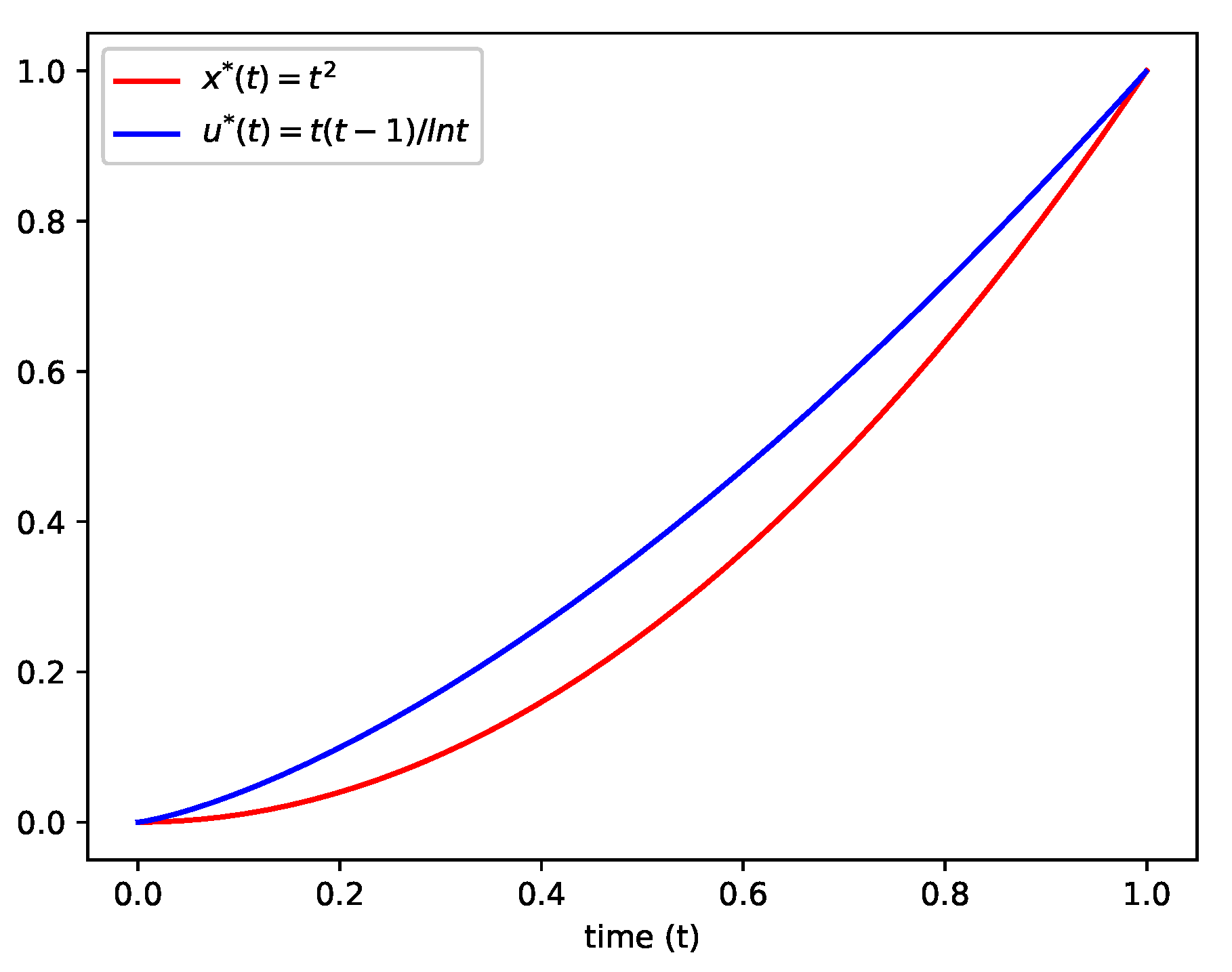
Example 1.
The triple given by , , and , for , is an extremal of the following distributed-order fractional optimal control problem:
Indeed, by defining the Hamiltonian function as
it follows:
- From the optimality condition ,
- From the adjoint equation ,
- From the transversality condition,
3.3. Sufficient Condition for Global Optimality
We now prove a Mangasarian type theorem for the distributed-order fractional optimal control problem (BP).
Theorem 2.
Consider the basic distributed-order fractional optimal control problem (BP). If and are concave and is a Pontryagin extremal with , , then
for any admissible pair .
Proof.
Because L is concave as a function of x and u, we have from Lemma 2 that
for any control u and its associated trajectory x. This gives
From the adjoint equation (2), we have
From the optimality condition (1), we know that
It follows from (12) that
Using the integration by parts formula of Lemma 1,
meaning that
Finally, taking into account that and f is concave in both x and u, we conclude that . □
Example 2.
4. Conclusions
In this paper we investigated fractional optimal control problems depending on distributed-order fractional operators. We have proven a necessary optimality condition of Pontryagin’s type and a Mangasarian-type sufficient optimality condition. The new results were illustrated with an example. As for future work, it would be interesting to develop proper numerical approaches to solve problems of optimal control with distributed-order fractional derivatives. In this direction, the approaches found in [17,18] can be easily adapted.
Author Contributions
The authors equally contributed to this paper, read and approved the final manuscript: Formal analysis, F.N. and D.F.M.T.; Investigation, F.N. and D.F.M.T.; Writing—original draft, F.N. and D.F.M.T.; Writing—review and editing, F.N. and D.F.M.T. All authors have read and agreed to the published version of the manuscript.
Funding
This research was funded by the Portuguese Foundation for Science and Technology (FCT), grant number UIDB/04106/2020 (CIDMA). Ndaïrou was also supported by FCT through the PhD fellowship PD/BD/150273/2019.
Acknowledgments
The authors are grateful to two anonymous reviewers for several comments and suggestions that have helped them to improve the manuscript.
Conflicts of Interest
The authors declare no conflict of interest.
References
- Caputo, M. Elasticità e Dissipazione; Zanichelli: Bologna, Italy, 1969. [Google Scholar]
- Caputo, M. Mean fractional-order-derivatives differential equations and filters. Ann. Univ. Ferrara Sez. VII 1995, 41, 73–84. [Google Scholar]
- Bagley, R.L.; Torvik, P.J. On the existence of the order domain and the solution of distributed order equations. I. Int. J. Appl. Math. 2000, 2, 865–882. [Google Scholar]
- Bagley, R.L.; Torvik, P.J. On the existence of the order domain and the solution of distributed order equations. II. Int. J. Appl. Math. 2000, 2, 965–987. [Google Scholar]
- Caputo, M. Distributed order differential equations modelling dielectric induction and diffusion. Fract. Calc. Appl. Anal. 2001, 4, 421–442. [Google Scholar]
- Diethelm, K.; Ford, N.J.; Freed, A.D.; Luchko, Y. Algorithms for the fractional calculus: A selection of numerical methods. Comput. Methods Appl. Mech. Engrg. 2005, 194, 743–773. [Google Scholar] [CrossRef] [Green Version]
- Atanackovic, T.M. A generalized model for the uniaxial isothermal deformation of a viscoelastic body. Acta Mech. 2002, 159, 77–86. [Google Scholar] [CrossRef]
- Lorenzo, C.F.; Hartley, T.T. Variable order and distributed order fractional operators. Nonlinear Dynam. 2002, 29, 57–98. [Google Scholar] [CrossRef]
- Mainardi, F.; Mura, A.; Pagnini, G.; Gorenflo, R. Time-fractional diffusion of distributed order. J. Vib. Control 2008, 14, 1267–1290. [Google Scholar] [CrossRef] [Green Version]
- Derakhshan, M.; Aminataei, A. Asymptotic Stability of Distributed-Order Nonlinear Time-Varying Systems with the Prabhakar Fractional Derivatives. Abstr. Appl. Anal. 2020, 2020, 1896563. [Google Scholar] [CrossRef]
- Van Bockstal, K. Existence and uniqueness of a weak solution to a non-autonomous time-fractional diffusion equation (of distributed order). Appl. Math. Lett. 2020, 109, 106540. [Google Scholar] [CrossRef]
- Zaky, M.A.; Machado, J.T. Multi-dimensional spectral tau methods for distributed-order fractional diffusion equations. Comput. Math. Appl. 2020, 79, 476–488. [Google Scholar] [CrossRef]
- Ali, M.S.; Shamsi, M.; Khosravian-Arab, H.; Torres, D.F.M.; Bozorgnia, F. A space-time pseudospectral discretization method for solving diffusion optimal control problems with two-sided fractional derivatives. J. Vib. Control 2019, 25, 1080–1095. [Google Scholar] [CrossRef]
- Nemati, S.; Lima, P.M.; Torres, D.F.M. A numerical approach for solving fractional optimal control problems using modified hat functions. Commun. Nonlinear Sci. Numer. Simul. 2019, 78, 104849. [Google Scholar] [CrossRef] [Green Version]
- Sidi Ammi, M.R.; Torres, D.F.M. Optimal control of a nonlocal thermistor problem with ABC fractional time derivatives. Comput. Math. Appl. 2019, 78, 1507–1516. [Google Scholar] [CrossRef] [Green Version]
- Almeida, R.; Morgado, M.L. The Euler-Lagrange and Legendre equations for functionals involving distributed-order fractional derivatives. Appl. Math. Comput. 2018, 331, 394–403. [Google Scholar] [CrossRef]
- Zaky, M.A.; Machado, J.A.T. On the formulation and numerical simulation of distributed-order fractional optimal control problems. Commun. Nonlinear Sci. Numer. Simul. 2017, 52, 177–189. [Google Scholar] [CrossRef]
- Zaky, M.A. A Legendre collocation method for distributed-order fractional optimal control problems. Nonlinear Dyn. 2018, 91, 2667–2681. [Google Scholar] [CrossRef]
- Almeida, R.; Pooseh, S.; Torres, D.F.M. Computational Methods in the Fractional Calculus of Variations; Imperial College Press: London, UK, 2015. [Google Scholar] [CrossRef]
- Samko, S.G.; Kilbas, A.A.; Marichev, O.I. Fractional Integrals and Derivatives; Gordon and Breach Science Publishers: Yverdon, Switzerland, 1993. [Google Scholar]
- Rockafellar, R.T. Convex Analysis; Princeton University Press: Princeton, NJ, USA, 1970. [Google Scholar]
- Ye, H.; Gao, J.; Ding, Y. A generalized Gronwall inequality and its application to a fractional differential equation. J. Math. Anal. Appl. 2007, 328, 1075–1081. [Google Scholar] [CrossRef] [Green Version]
- Cao, L.; Li, Y.; Tian, G.; Liu, B.; Chen, Y. Time domain analysis of the fractional order weighted distributed parameter Maxwell model. Comput. Math. Appl. 2013, 66, 813–823. [Google Scholar] [CrossRef]
- Pontryagin, L.S.; Boltyanskii, V.G.; Gamkrelidze, R.V.; Mishchenko, E.F. The Mathematical Theory of Optimal Processes; A Pergamon Press Book; The Macmillan Co.: New York, NY, USA, 1964. [Google Scholar]
- Reid, W.T. Ramifications of the fundamental lemma of the calculus of variations. Houst. J. Math. 1978, 4, 249–262. [Google Scholar]
Figure 1.
The optimal control and corresponding optimal state variable , solution of problem (7).
Figure 1.
The optimal control and corresponding optimal state variable , solution of problem (7).

Publisher’s Note: MDPI stays neutral with regard to jurisdictional claims in published maps and institutional affiliations. |
© 2020 by the authors. Licensee MDPI, Basel, Switzerland. This article is an open access article distributed under the terms and conditions of the Creative Commons Attribution (CC BY) license (http://creativecommons.org/licenses/by/4.0/).
Share and Cite
MDPI and ACS Style
Ndaïrou, F.; Torres, D.F.M. Distributed-Order Non-Local Optimal Control. Axioms 2020, 9, 124. https://0-doi-org.brum.beds.ac.uk/10.3390/axioms9040124
AMA Style
Ndaïrou F, Torres DFM. Distributed-Order Non-Local Optimal Control. Axioms. 2020; 9(4):124. https://0-doi-org.brum.beds.ac.uk/10.3390/axioms9040124
Chicago/Turabian StyleNdaïrou, Faïçal, and Delfim F. M. Torres. 2020. "Distributed-Order Non-Local Optimal Control" Axioms 9, no. 4: 124. https://0-doi-org.brum.beds.ac.uk/10.3390/axioms9040124
Note that from the first issue of 2016, this journal uses article numbers instead of page numbers. See further details here.