Bitcoin Analysis and Forecasting through Fuzzy Transform

Abstract

Sentiment analysis to characterize the properties of Bitcoin prices and their forecasting is here developed thanks to the capability of the Fuzzy Transform (F-transform for short) to capture stylized facts and mutual connections between time series with different natures. The recently proposed L_p-norm F-transform is a powerful and flexible methodology for data analysis, non-parametric smoothing and for fitting and forecasting. Its capabilities are illustrated by empirical analyses concerning Bitcoin prices and Google Trend scores (six years of daily data): we apply the (inverse) F-transform to both time series and, using clustering techniques, we identify stylized facts for Bitcoin prices, based on (local) smoothing and fitting F-transform, and we study their time evolution in terms of a transition matrix. Finally, we examine the dependence of Bitcoin prices on Google Trend scores and we estimate short-term forecasting models; the Diebold–Mariano (DM) test statistics, applied for their significance, shows that sentiment analysis is useful in short-term forecasting of Bitcoin cryptocurrency.

1. Introduction

The notion of a fuzzy transform (F-transform) as a tool for modeling with fuzzy rules as specific transformation and for general approximation of functions has been introduced by Perfilieva in [1] (see also [2]) and is now recognized as a powerful technique with important properties and potentials for various applications, as developed in several papers and special issues (see, e.g, [3,4,5] and the references therein).

In the present paper, we will focus on the use of quantile and expectile F-transform (and, more generally, on $L_p$-norm-based fuzzy-valued F-transforms) in modeling time series. In particular, we will show the application of direct and inverse $L_p$-norm F-transform to analyze the connection between Bitcoin returns and the level of interest in the world wide web. The Bitcoin observed time series is modeled through fuzzy-valued functions, whose level-cuts can be interpreted in the setting of expectile and quantile fuzzy regressions; these last are introduced in [6,7] as non-parametric smoothing methodologies and are constructed by defining fuzzy-valued $L_p$-norm extensions of the F-transforms (in particular, expectile or $L_2$-norm and quantile or $L_1$-norm).

Quantile regression is also applied in [8] to show that Bitcoin reacts positively to uncertainty at both higher quantiles and shorter frequency movements of Bitcoin returns.

Following recent research on financial time series, where the properties of quantile and expectile modeling are discussed with respect to coherent and elicitable risk measures (see [9,10]), expectile methods seem to compete favourably with quantiles; furthermore, some recent papers (e.g., [11]) suggest to adopt $L_p$-norm-based procedures with p between 1 and 2 (e.g., $p\in \left\{1.25,1.5,1.75\right\}$), in order to consider (probabilistic) tail behaviour according, e.g., to robust Extreme Value Theory.

Literature about Bitcoin has hugely grown in recent years and some papers deserve a citation. An exhaustive analysis of Bitcoin and its statistical properties are explored in [12] by a comparison with standard currencies dynamics. Yermack in [13] shows that Bitcoin does not satisfy the three main properties called medium of exchange, unit of account and store of value, concluding that it is not a currency but rather a speculative asset. However, a debate is still open about the nature of Bitcoin and many hints can be found in [14,15,16]. A shared property by financial instruments is the day-of-the-week effect and in [17] the same effect is proved for Bitcoin returns and volatility through OLS and GARCH model. The possibility of global economic policy uncertainty to produce valid information to improve the prediction of returns and volatility in the Bitcoin market is detailed in [18].

Research on possible forecasting models to be used as decision support tools in investment strategies is more recent; in [19], monthly data are considered and it is shown that the predictive ability of the internet-based economic uncertainty related queries index is statistically stronger than the measure of uncertainty derived from newspapers in predicting Bitcoin returns.

The nexus between Bitcoin prices and market sentiment is further studied in many papers: in [20] sentiment is shown to explain about 2.5% to 5% of the unusual level of price clustering in Bitcoin. In [21] the cross-correlations between Google Trends and Bitcoin market is analyzed through the Multifractal Detrended Cross-correlation Analysis (MF-DCCA) method and in [22], within the more general context of Dow Jones Industrial Average, it is shown that Google searches are power-law correlated with Hurst exponents between 0.8 and 1.1; the authors conclude that globally on time domain, there is no relationship between the on-line search queries and some financial measures. In [23] investor sentiment regarding Bitcoin is introduced because of its significant information for explaining changes in Bitcoin volatility for future periods; on this basis Bitcoin is proved to be an investment asset with high volatility and dependence on investor sentiment rather than a monetary asset.

In a more general framework, in [24], interactions between (mass) media reporting and financial market movements are measured with particular focus on the property of sentiment as a predictors of securities prices.

The existing high correlation between Bitcoin prices and Google Trend scores is discovered and documented since the origins of digital currencies (see, e.g., [25]) and several pieces of research have discussed about its characteristics (see [26]) and about predicting prices using sentiment analysis (see references numbered from 23 to 27 in [26]). On the other hand, there is evidence that a bi-directional causal relationship exists between Bitcoin web-attention and Bitcoin returns, in particular for data in the left tail (poor performance) and the right tail (superior performance) of the observed statistical distribution (see [27]).

A non-parametric forecasting model based on technical analysis is presented in [28], focusing on the presence of predictive local non-linear trends that reflect the speculative nature of cryptocurrency trading. In [29] a computational intelligence technique that uses a hybrid Neuro-Fuzzy controller is introduced to forecast the direction in the change of the daily price of Bitcoin and its performance is shown to be good when compared with two other computational intelligence models based on a simpler neuro-fuzzy model and an artificial neural network.

Forecasting of Bitcoin risk measures is developed in [30] by comparing predictability of the one-step-ahead volatility with Value-at-Risk using several volatility models.

Many other authors approach general cryptocurrency properties. For example, in [31] there is evidence that Bitcoin is the most influential among digital coins both as a transmitter toward digital currencies and as a receiver of spillovers from virtual and traditional instruments. An extended analysis is also presented in [32] where the four cryptocurrencies Bitcoin, Ethereum, Ripple and Litecoin are predicted through a combination of eight models revealing that a combination of stochastic volatility and a student-t distribution gives the best results. The same topic of Bitcoin-realized volatility forecasting is studied in [33] where conventional regression models are substituted by least-squares model-averaging methods and no investor sentiment is modeled.

In [34,35] a continuous time model for Bitcoin price dynamics is studied to detect bubbles; regarding the existence of a bubble, in [36] it is proved it holds from early 2013 to mid-2014, but, not in late 2017 as supposed. Evidence of bubbly Bitcoin behaviour, mainly in the 2017–2018 period, is shown in [37], where it is also proved that economic policy uncertainty and stock market volatility play the most important role in Bitcoin values.

The evidence for the Bitcoin bubble is confirmed in [38] through the empirical validation of three properties: volume of trading is mainly explained in terms of price dynamics, trading is based exclusively on past prices and the price of Bitcoin is an explosive process.

In [39] a thorough analysis is conducted: several alternative univariate and multivariate models for point and density forecasting of crypto-series are compared, finding statistically significant improvements in point forecasting when using combinations of univariate models, and in density forecasting when relying on the selection of multivariate models.

Various deep learning-based Bitcoin price prediction models are studied in [40] using Bitcoin block-chain information; regression and classification problems are addressed in the sense that the first predicts the future Bitcoin price and the second one predicts whether the future price will go up or down.

In the case of Bitcoin prices using high frequency data, in [41] it is shown that it exists a large degree of multi-fractality in all examined time intervals which can be attributed to the high kurtosis and the fat distributional tails of the series returns; in [42] there is evidence about the leverage effect as the most powerful effect in volatility forecasting; volatility is also analyzed in [43] in terms of the property of the long memory parameter to be significant and quite stable for both unconditional and conditional volatilities at different time scales. Extending the study to several high frequency cryptocurrencies data, in [44] the investigation on stylized facts is developed in terms of the Hurst exponent of dependence between four different cryptocurrencies.

Also in [45] multi-fractality of Bitcoin time series is investigated, confirming that both temporal correlation and the fat-tailed distribution are the main sources, in addition in [46] a possible use of multi-fractal parameters in Technical Analysis is suggested.

The paper is organized into six sections. Preliminary facts on our methodology concerning F-transform are presented in section two. Our empirical experiments and analyses concerning Bitcoin prices and Google Trend scores are detailed in sections three and four: in section three, we apply the expectile and quantile (inverse) F-transforms to both time series and we examine their relationship on pre-clustered subsets of observations, subdivided in terms of three different clustering criteria; in section four we identify stylized facts for Bitcoin prices, based on local (low-order polynomial) trends obtained by direct F-transform, we study their clustering to obtain (centroid) typical forms and we use them to reconstruct the time series and to analyze their time evolution in terms of a transition matrix. Possible short-term forecasting models of Bitcoin prices using Google Trends are shown in section five and the Diebold–Mariano (DM) test statistics is applied for their significance. Section six closes with some comments and hints for future research paths.

2. Fuzzy-Transform Smoothing

We introduced in [47] and then we enhance in [6] two non-parametric smoothing methodologies called expectile and quantile fuzzy-transform; the first one is based on the classical direct F-transform and it is obtained by minimizing a least-squares (L₂-norm) operator while the second one is based on the L₁-type direct F-transform and it is obtained by minimizing an L₁-norm operator.

Some preliminary notions compose the research framework: a fuzzy set is a mapping $u:\mathbb{R}⟶[0, 1]$ and a fuzzy interval is a fuzzy set on $\mathbb{R}$ with the properties that the mapping u is (i) normal ($\exists \widehat{x}\in \mathbb{R}$ with $u(\widehat{x})=1$), (ii) upper semi-continuous, (iii) fuzzy convex ($u(\lambda x^{\prime }+(1-\lambda )x^{″})\ge$ $\min \{u(x^{\prime }),u(x^{″})\}$ for all $\lambda \in [0, 1]$), (iv) $cl\{x|u(x)>0\}$ is a compact interval. A consequence of (ii) and (iii) is that the α-cuts ${\left[u\right]}_{\alpha }=\left\{x\right|u\left(x\right)\ge \alpha \}=[u_{\alpha }^{-},u_{\alpha }^{+}]$ are compact intervals for all $\alpha \in [0, 1]$. The 1-cut is the core ${\left[u\right]}_1=\left\{x\right|u\left(x\right)=1\}$ of u; the interval ${\left[u\right]}_0=$$cl\left(\right\{x\left|u\right(x)>0\})$ is the 0-cut of u. A fuzzy interval is a fuzzy number if its core is a singleton ${\left[u\right]}_1=\left\{\widehat{u}\right\}$ with $\widehat{u}\in \mathbb{R}$.

The space of real fuzzy intervals is denoted ${\mathbb{R}}_{\mathcal{F}}$ and the mapping $u\in {\mathbb{R}}_{\mathcal{F}}$ satisfies what follows:

$$u\left(x\right)=\left\{\begin{array}{ccc}0& \mathrm{if}& x\notin {\left[u\right]}_0\\ \sup \left\{\alpha \right|x\in {\left[u\right]}_{\alpha }\}& \mathrm{if}& x\in {\left[u\right]}_0.\end{array}\right.$$

(1)

For a given real compact interval $[a,b]$, a generalized r-partition is defined by a triplet $(\mathbb{P},\mathbb{A},r)$ where $r\ge 1$ is integer, $\mathbb{P}=\left\{x_j=a+\frac{j-1}{n-1}(b-a);j=1,2, \dots , n\right\}$, $n\ge 2$, is a uniform decomposition of $[a,b]$; for simplicity of notation, if $r>1$ we extend $\mathbb{P}$ by adding $r-1$ points $x_{1-j}=a-j\frac{b-a}{n-1},j=1, \dots , r-1$ on the left of a and $r-1$ points $x_{n+j}=b+j\frac{b-a}{n-1},j=1, \dots , r-1$ on the right of b. The second term of the triplet is a family $\mathbb{A}=\{A_{-r+2}, \dots , A_1, A_2, \dots , A_n, \dots , A_{n+r-1}\}$ of $n+2r-2$ continuous fuzzy sets on $\mathbb{R}$, called basic functions, that satisfy the following condition for all $x\in [a,b]$

$$\sum _{k=-r+2}^{n+r-1}{A}_k\left(x\right)=r$$

(2)

and are such that $A_k\left(x_k\right)=1$, for $k=2-r, \dots ,1, 2, \dots , n, \dots , n+r-1$, $A_k\left(x\right)=0$ for all $x\notin [x_{k-r},x_{k+r}]$.

If $r=1$, the partition $(\mathbb{P},\mathbb{A},1)$ will be simply denoted by $(\mathbb{P},\mathbb{A})$.

Families of basic functions can be obtained in terms of increasing shape functions such as rational splines of the form

$$L(t;{\beta }_0,{\beta }_1)=\frac{t^2+{\beta }_{0}t(1-t)}{1+({\beta }_0+{\beta }_1-2)t(1-t)}, t\in [0, 1]$$

(3)

with real parameters ${\beta }_0\ge 0$, ${\beta }_1\ge 0$; the Hermite-type conditions $L\left(0\right)=0$, $L\left(1\right)=1$, $L^{\prime }\left(0\right)={\beta }_0$, $L^{\prime }\left(1\right)={\beta }_1$ are satisfied and $L^{\prime }\left(t\right)\ge 0$ for all $t\in [0, 1]$. By any pair of non-negative values ${\beta }_0$, ${\beta }_1$, a large number of shape functions can be generated; for example, if ${\beta }_0+{\beta }_1=2$ (with $0\le {\beta }_0\le 2$, ${\beta }_1=2-{\beta }_0$) we have a quadratic function $L\left(t\right)=(1-{\beta }_0)t^2+{\beta }_{0}t$, e.g., $L(t;2,0)=2t-t^2$, $L(t;0,2)=t^2$ and $L(t;1,1)=t$ is linear.

Each basic function $A_k$, $k=2-r, \dots , 1, 2, \dots , n, \dots , n+r-1$, increasing on $\left[x_{k-r},x_k\right]$ and decreasing on $\left[x_k,x_{k+r}\right]$, is obtained by translating $t\to L(t,{\beta }_0,{\beta }_1)$ and $t\to L(1-t,{\beta }_0,{\beta }_1)$ from $[0,1]$ onto $\left[x_{k-r},x_k\right]$ and $\left[x_k,x_{k+r}\right]$, respectively (each $A_k$ is finally extended to $\mathbb{R}$ by setting $A_k\left(x\right)=0$ on the left of $x_{k-r}$ and on the right of $x_{k+r}$).

2.1. L₂-Norm F-Transform in Expectile Smoothing

We just recall the discrete version of the direct F-transform.

Definition 1.

(from [1]) Given a set of m values $\mathit{Y}=\left\{(t_i,f_i)|t_i\in [a,b],i=1, \dots , m\right\}$ of a function $f:[a,b]⟶\mathbb{R}$ and a fuzzy partition $(\mathbb{P},\mathbb{A})$ of $[a,b]$ such that each subinterval $[x_{k-1},x_{k+1}]$ contains at least one point $t_i$ in its interior (so that ${\sum }_{i=1}^m{A}_k\left(t_i\right)>0$ for all k), then the discrete direct $L_2$-type F-transform of $\mathit{Y}$ with respect to $(\mathbb{P},\mathbb{A})$ is the n-tuple of real numbers $(F_1, \dots , F_n)$ where each component $F_k$ minimizes the function ${\mathsf{\Phi }}_k\left(y\right)={\displaystyle \sum _{i=1}^m}{|f_i-y|}^2{A}_k\left(t_i\right)$, $k=1,2,\dots ,n$. The associated inverse F-transform function (iF-transform for short) is defined by ${\widehat{f}}_{(\mathbb{P},\mathbb{A})}\left(x\right)={\displaystyle \sum _{k=1}^n}{F}_k{A}_k\left(x\right)$ for all $x\in [a,b]$.

More generally, we consider a r-partition $(\mathbb{P},\mathbb{A},r)$ and substitute the direct F-transform components $F_k$, with an $(n+2r-2)$-tuple of polynomials of order $q\ge 0$, say $({\phi }_{2-r}\left(x\right), \dots , {\phi }_{n+r-1}\left(x\right))$ with ${\phi }_k\left(x\right)=F_{k,0}+F_{k,1}(x-x_k)+ \dots +F_{k,q}{(x-x_k)}^q$, $k=2-r, \dots , n+r-1$. The $q+1$ coefficients $F_{k,j},j=0, 1, \dots , q$ are obtained, for fixed k, by minimizing the function ${\mathsf{\Phi }}_k(y_0, \dots , y_q)={\displaystyle {\displaystyle \sum _{i=1}^m}}{|f_i-\left(y_0+y_1(t_i-x_k)+ \dots +y_q{(t_i-x_k)}^q\right)|}^2{A}_k\left(t_i\right)$ with respect to the parameters $y_0, \dots , y_q$, under the assumption that for each k, the data points $(t_i,f_i)$ with $t_i$ in the interval $\left[x_{max(a,k-r)},x_{min(b,k+r)}\right]$ produce a unique optimal solution. The details are shown in [6].

The corresponding (inverse) iF-transform function is given by

$${\widehat{f}}_{(\mathbb{P},\mathbb{A},r)}^{\left(q\right)}\left(x\right)=\frac{1}{r}\sum _{k=2-r}^{n+r-1}{A}_k\left(x\right){\phi }_k(x;F_{k,0}, \dots , F_{k,q}) for x\in [a,b].$$

(4)

Consider for simplicity the F-transform of order zero ($q=0$).

The iF-transform function becomes

$${\widehat{f}}_{(\mathbb{P},\mathbb{A},r)}\left(x\right)=\frac{1}{r}\sum _{k=2-r}^{n+r-1}{F}_k{A}_k\left(x\right) for x\in [a,b]$$

(5)

with the $(n+2r-2)$-tuple of the direct F-transform $(F_{2-r}, \dots , F_{n+r-1})$.

We recall from [6] that the expectile direct F-transform components are defined to be the minimizers of the strictly convex functions, for $k=2-r, \dots , 1, \dots , n, \dots , n+r-1$ and $\omega \in [0,1]$,

$${\mathsf{\Phi }}_{k,\omega }(\mu )=\sum _{j=1}^m{w}_j(\omega ;\mu ){(f_j-\mu )}^2{A}_k(t_j)$$

(6)

where

$$w_j(\omega ;\mu )=\left\{\begin{array}{ccc}\omega & \mathrm{if}& f_j>\mu \\ 1-\omega & \mathrm{if}& f_j\le \mu \end{array}\right..$$

(7)

The value ${\mu }_k={\mu }_k\left(\omega \right)$ (depending on ω) is the expectile for the asymmetry parameter $\omega \in [0, 1]$ and if $\omega =\frac{1}{2}$ we obtain the direct F-transform component $F_k$ in Equation (5).

Proposition 1.

([6]) Given the set of minimizers $\left\{{\mu }_k\left(\omega \right)\right|\omega \in ]0,1\left[\right\}$ of ${\mathsf{\Phi }}_{k,\omega }\left(\mu \right)$, consider $\alpha \in [0,1]$; then the compact intervals

$$U_{k,\alpha }=\left\{\begin{array}{ccc}\left\{{\mu }_k\right(\frac{1}{2}\left)\right\}\hfill & if& \alpha =1\\ \left[{\mu }_k\right(\frac{\alpha }{2}),{\mu }_k(1-\frac{\alpha }{2}\left)\right]\hfill & if& \alpha \in ]0, 1[\\ cl\left({\displaystyle \bigcup _{\beta >0}}{U}_{k,\beta }\right)\hfill & if& \alpha =0\end{array}\right.$$

(8)

define the α-cuts of a fuzzy number$u_k\in {\mathbb{R}}_{\mathcal{F}}$with membership function

$$u_k\left(x\right)=\left\{\begin{array}{ccc}\sup \left\{\alpha \right|x\in U_{k,\alpha }\}\hfill & \mathit{if}& x\in U_{k,0}\\ 0\hfill & \mathit{if}& x\notin U_{k,0}\end{array}\right..$$

(9)

Definition 2.

Given a set of m points $Y=\{(t_i,f_i);$ $t_i\in [a,b]$, $i=1, \dots , m\}$ and a fuzzy r-partition $(\mathbb{P},\mathbb{A},r)$ of $[a,b]$, the ($n+2r-2$)-vector of fuzzy numbers

$${\mathbf{F}}_{(\mathbb{P},\mathbb{A},r)}=(F_{2-r}, \dots , F_{n+r-1}),$$

(10)

where each fuzzy interval $F_k$ has α-cuts $U_{k,\alpha }$ given by (8) in Proposition 1, is called the discrete direct expectile fuzzy-valued F-transform of f with respect to $(\mathbb{P},\mathbb{A},r)$, based on the dataset Y. The corresponding inverse expectile fuzzy-valued iF-transform is the fuzzy-valued function defined by

$${\widehat{f}}_{(\mathbb{P},\mathbb{A},r)}\left(x\right)=\frac{1}{r}\sum _{k=2-r}^{n+r-1}{F}_k{A}_k(x) for x\in [a,b].$$

(11)

The fuzzy-valued function ${\widehat{f}}_{(\mathbb{P},\mathbb{A},r)}(x)$ is well defined as indeed each basic function $A_k$ has non-negative values for each $x\in [a,b]$. The $\alpha$-cuts $U_{k,\alpha }$ of $F_k$ will be denoted by

$${\left[F_k\right]}_{\alpha }=[F_{k,\alpha }^{-},F_{k,\alpha }^{+}], k=2-r, \dots , n+r-1, \alpha \in [0,1]$$

(12)

and the $\alpha$-cuts of the fuzzy-valued function ${\widehat{f}}_{(\mathbb{P},\mathbb{A},r)}\left(x\right)$, $x\in [a,b]$, will be given by

$${\left[{\widehat{f}}_{(\mathbb{P},\mathbb{A},r)}\left(x\right)\right]}_{\alpha }=\left[\frac{1}{r}\sum _{k=2-r}^{n+r-1}{F}_{k,\alpha }^{-}{A}_k\left(x\right),\frac{1}{r}\sum _{k=2-r}^{n+r-1}{F}_{k,\alpha }^{+}{A}_k\left(x\right)\right], \alpha \in [0,1].$$

(13)

When $\alpha =1$ we obtain the standard direct $F-$transform and the standard $iF-$transform function, corresponding to the core of the fuzzy-valued iF-transform.

2.2. L₁-Norm F-Transform in Quantile Smoothing

The L₁-norm direct and inverse F-transform are defined as follows.

Definition 3.

Given a set of m values $\mathit{Y}=\left\{(t_i,f_i)|t_i\in [a,b],i=1, \dots , m\right\}$ of a function $f:[a,b]⟶\mathbb{R}$ and a fuzzy partition $(\mathbb{P},\mathbb{A})$ of $[a,b]$ such that each subinterval $[x_{k-1},x_{k+1}]$ contains at least one point $t_i$ in its interior, then the discrete direct $L_1$-type F-transform of $\mathit{Y}$ with respect to $(\mathbb{P},\mathbb{A})$ is the n-tuple of real numbers $(G_1, \dots , G_n)$ where each component $G_k$ minimizes the function ${\mathsf{\Psi }}_k\left(y\right)={\displaystyle \sum _{i=1}^m}\left|f_i-y\right|A_k\left(t_i\right)$, $k=1, 2, \dots , n$. The associated inverse F-transform function (iF-transform for short) is defined by ${\tilde{f}}_{(\mathbb{P},\mathbb{A})}\left(x\right)={\displaystyle \sum _{k=1}^n}{G}_k{A}_k\left(x\right)$ for all $x\in [a,b]$.

Also in this case, we consider a generalized r-partition $(\mathbb{P},\mathbb{A},r)$ and substitute the direct F-transform components $G_k$ with an $(n+2r-2)$-tuple of polynomials of order $q\ge 0$, say $({\psi }_{2-r}\left(x\right), \dots , {\psi }_{n+r-1}\left(x\right))$ with ${\psi }_k\left(x\right)=G_{k,0}+G_{k,1}(x-x_k)+ \dots +G_{k,q}{(x-x_k)}^q$, $k=2-r, \dots , n+r-1$. The $q+1$ coefficients $G_{k,j},j=0, 1, \dots , q$ are obtained, for fixed k, by minimizing the function ${\mathsf{\Psi }}_k(y_0, \dots , y_q)={\displaystyle \sum _{i=1}^m}\left|f_i-\left(y_0+y_1(t_i-x_k)+ \dots +y_q{(t_i-x_k)}^q\right)\right|A_k\left(t_i\right)$ with respect to the parameters $y_0, \dots , y_q$ (see details in [6]).

The corresponding $L_1$-type inverse F-transform function is given by

$${\stackrel{\sim }{f}}_{(\mathbb{P},\mathbb{A},r)}^{\left(q\right)}\left(x\right)=\frac{1}{r}\sum _{k=2-r}^{n+r-1}{A}_k\left(x\right){\psi }_k(x;G_{k,0}, \dots , G_{k,q}) for x\in [a,b].$$

(14)

The iF-transform function of order zero ($p=0$) becomes

$${\stackrel{\sim }{f}}_{(\mathbb{P},\mathbb{A},r)}\left(x\right)=\frac{1}{r}\sum _{k=2-r}^{n+r-1}{G}_k{A}_k\left(x\right) for x\in [a,b]$$

(15)

with the $(n+2r-2)$-tuple of the $L_1$-type direct F-transform $(G_{2-r}, \dots , G_{n+r-1})$.

We recall from [6] that the quantile direct F-transform is defined in terms of the minimizers of the convex functions, for $k=1, \dots , n$ and $\omega \in [0,1]$,

$${\mathsf{\Psi }}_{k,\omega }\left(\eta \right)=\sum _{j=1}^m{w}_j\left(\omega ;\eta \right)\left|f_j-\eta \right|A_k\left(t_j\right)$$

(16)

where

$$w_j\left(\omega ;\eta \right)=\left\{\begin{array}{ccc}\omega & \mathrm{if}& f_j>\eta \\ 1-\omega & \mathrm{if}& f_j\le \eta \end{array}\right..$$

(17)

As detailed in [6], the minimization of ${\mathsf{\Psi }}_{k,\omega }\left(\eta \right)$ produces the family of compact intervals, for $\alpha \in [0,1]$ and $\omega \in \left\{\frac{\alpha }{2},1-\frac{\alpha }{2}\right\}$ ,

$$V_{k,\alpha }=\left\{\begin{array}{ccc}\left\{{\eta }_k\left(\frac{1}{2}\right)\right\}\hfill & \mathrm{if}& \alpha =1\\ \left[{\eta }_k\left(\frac{\alpha }{2}\right),{\eta }_k\left(1-\frac{\alpha }{2}\right)\right]\hfill & \mathrm{if}& \alpha \in [0,1]\\ cl\left({\displaystyle \bigcup _{\beta >0}}{V}_{k,\beta }\right)\hfill & \mathrm{if}& \alpha =0;\end{array}\right.$$

(18)

and we obtain the $\alpha$-cuts of a fuzzy number $v_k\in {\mathbb{R}}_{\mathcal{F}}$ with membership function

$$v_k\left(x\right)=\left\{\begin{array}{ccc}sup\left\{\alpha \right|x\in V_{k,\alpha }\}\hfill & \mathrm{if}& x\in V_{k,0}\\ 0\hfill & \mathrm{if}& x\notin V_{k,0}.\end{array}\right.$$

(19)

Definition 4.

Given a set of m points $Y=\{(t_i,f_i);$ $t_i\in [a,b]$, $i=1, \dots , m\}$ and a fuzzy r-partition $(\mathbb{P},\mathbb{A},r)$ of $[a,b]$, the ($n+2r-2$)-vector of fuzzy numbers

$${\mathbf{G}}_{(\mathbb{P},\mathbb{A},r)}=(G_{2-r}, \dots , G_{n+r-1}),$$

(20)

where each fuzzy interval $G_k$ has α-cuts $V_{k,\alpha }$, is called the discrete direct quantile fuzzy transform of Y with respect to $(\mathbb{P},\mathbb{A},r)$.

The corresponding (inverse) quantile iF-transform of f is the fuzzy-valued function defined by

$${\stackrel{\sim }{f}}_{(\mathbb{P},\mathbb{A},r)}\left(x\right)=\frac{1}{r}\sum _{k=2-r}^{n+r-1}{G}_k{A}_k\left(x\right) \mathrm{for}x\in [a,b].$$

(21)

Denoting the $\alpha$-cuts $V_{k,\alpha }$ of $G_k$ by

$${\left[G_k\right]}_{\alpha }=\left[G_{k,\alpha }^{-},G_{k,\alpha }^{+}\right], k=2-r, \dots , n+r-1, \alpha \in [0,1],$$

(22)

then, the $\alpha$-cuts of the corresponding fuzzy-valued function ${\tilde{f}}_{(\mathbb{P},\mathbb{A},r)}\left(x\right)$, $x\in [a,b]$, will be given by

$${\left[{\stackrel{\sim }{f}}_{(\mathbb{P},\mathbb{A},r)}\left(x\right)\right]}_{\alpha }=\left[\frac{1}{r}\sum _{k=2-r}^{n+r-1}{G}_{k,\alpha }^{-}{A}_k\left(x\right),\frac{1}{r}\sum _{k=2-r}^{n+r-1}{G}_{k,\alpha }^{+}{A}_k\left(x\right)\right], \alpha \in [0,1].$$

(23)

2.3. General L_p-Norm-Based Discrete F-Transform

The general $L_p$-norm-based F-transform has been analyzed in detail in [48] for the continuous case. Its interest in time series applications is motivated by recent literature on tail behaviour of economic and financial time series (see, e.g., [11]) and in modeling risk measures ([9,10]): $L_p$-norm estimation with $1<p<2$ has been suggested to balance robustness and fitting properties.

For a dataset of m values $\mathbf{Y}=\left\{(t_i,f_i)|t_i\in [a,b],i=1, \dots , m\right\}$ and a generalized r-partition $(\mathbb{P},\mathbb{A},r)$, the $L_p$-norm direct F-transform is an $(n+2r-2)$-tuple of polynomials of order $q\ge 0$ $({\vartheta }_{2-r}\left(x\right), \dots , {\vartheta }_{n+r-1}\left(x\right))$ with ${\vartheta }_k\left(x\right)={\theta }_{k,0}+{\theta }_{k,1}(x-x_k)+ \dots +{\theta }_{k,q}{(x-x_k)}^q$, $k=2-r, \dots , n+r-1$, where this time, the $q+1$ coefficients ${\theta }_{k,j},j=0,1, \dots , q$, are obtained by minimizing the functions ${\Theta }_k^{\left(p\right)}({\theta }_0, \dots , {\theta }_q)={\displaystyle \sum _{i=1}^m}{\left|f_i-\left({\theta }_0+{\theta }_1(t_i-x_k)+ \dots +{\theta }_q{(t_i-x_k)}^q\right)\right|}^p{A}_k\left(t_i\right)$ with respect to the parameters ${\theta }_0, \dots , {\theta }_q$.

If $q=0$, the direct fuzzy-valued F-transform components, for a fixed $p\in [1,2]$, are obtained by minimizing the strictly convex functions, for $k=2-r, \dots , 1, \dots , n, \dots , n+r-1$ and $\omega \in [0,1]$,

$${\Theta }_{k,\omega }^{\left(p\right)}\left(\theta \right)=\sum _{j=1}^m{w}_j\left(\omega ;\theta \right){\left|f_j-\theta \right|}^p{A}_k\left(t_j\right)$$

(24)

where

$$w_j\left(\omega ;\theta \right)=\left\{\begin{array}{ccc}\omega & \mathrm{if}& f_j>\theta \\ 1-\omega & \mathrm{if}& f_j\le \theta \end{array}\right..$$

(25)

The minimizers ${\vartheta }_k={\vartheta }_k\left(\omega \right)$ (depending on $\omega$) define the $L_p$-norm direct F-transform components for the asymmetry parameter $\omega \in [0,1]$. We have (the proof is similar to the case $p=2$ in [6])

Proposition 2.

Given the set of minimizers $\left\{{\vartheta }_k\left(\omega \right)|\omega \in [0,1]\right\}$ of ${\Theta }_{k,\omega }^{\left(p\right)}\left(\theta \right)$, consider $\alpha \in [0,1]$; then, the compact intervals

$$W_{k,\alpha }=\left\{\begin{array}{ccc}\left\{{\theta }_k\left(\frac{1}{2}\right)\right\}\hfill & \mathit{if}& \alpha =1\\ \left[{\theta }_k\left(\frac{\alpha }{2}\right),{\theta }_k\left(1-\frac{\alpha }{2}\right)\right]\hfill & \mathit{if}& \alpha \in [0,1]\\ cl\left({\displaystyle \bigcup _{\beta >0}}{W}_{k,\beta }\right)\hfill & \mathit{if}& \alpha =0\end{array}\right.$$

(26)

define the α-cuts of a fuzzy number $w_k\in {\mathbb{R}}_{\mathcal{F}}$ with membership function

$$w_k\left(x\right)=\left\{\begin{array}{ccc}\sup \left\{\alpha \right|x\in W_{k,\alpha }\}\hfill & \mathit{if}& x\in W_{k,0}\\ 0\hfill & \mathit{if}& x\notin W_{k,0}\end{array}\right..$$

(27)

Definition 5.

Given a set of m points $Y=\{(t_i,f_i);$ $t_i\in [a,b]$, $i=1, \dots , m\}$ and a fuzzy r-partition $(\mathbb{P},\mathbb{A},r)$ of $[a,b]$, the ($n+2r-2$)-vector of fuzzy numbers

$${\mathbf{H}}_{(\mathbb{P},\mathbb{A},r)}=(H_{2-r}, \dots , H_{n+r-1}),$$

(28)

where each fuzzy interval $H_k$ has α-cuts $W_{k,\alpha }$ given by (26) in Proposition 2, is called the discrete direct $L_p$-norm fuzzy-valued F-transform with respect to $(\mathbb{P},\mathbb{A},r)$, based on the dataset Y. The corresponding inverse $L_p$-norm fuzzy-valued iF-transform is the fuzzy-valued function defined by

$$f_{(\mathbb{P},\mathbb{A},r)}^{\left(p\right)}\left(x\right)=\frac{1}{r}\sum _{k=2-r}^{n+r-1}{H}_k{A}_k\left(x\right) \mathit{for}x\in [a,b].$$

(29)

The $\alpha$-cuts $W_{k,\alpha }$ of $H_k$ will be denoted by

$${\left[H_k\right]}_{\alpha }=\left[H_{k,\alpha }^{-},H_{k,\alpha }^{+}\right], k=2-r, \dots , n+r-1, \alpha \in [0,1]$$

(30)

and the $\alpha$-cuts of the fuzzy-valued function $f_{(\mathbb{P},\mathbb{A},r)}^{\left(p\right)}\left(x\right)$, $x\in [a,b]$, are

$${\left[f_{(\mathbb{P},\mathbb{A},r)}^{\left(p\right)}\left(x\right)\right]}_{\alpha }=\left[\frac{1}{r}\sum _{k=2-r}^{n+r-1}{H}_{k,\alpha }^{-}{A}_k\left(x\right),\frac{1}{r}\sum _{k=2-r}^{n+r-1}{H}_{k,\alpha }^{+}{A}_k\left(x\right)\right], \alpha \in [0,1].$$

(31)

When $\alpha =1$ we obtain the $L_p$-norm direct F-transform and (inverse) iF-transform function, corresponding to the core of the fuzzy-valued $L_p$-norm iF-transform.

3. Analysis of Bitcoin Prices and Google Trends by F-Transform

To focus on the strength of fuzzy-valued $L_p$-norm F-transform smoothing, we will apply the proposed models to the time series of Bitcoin prices, which has received much attention by regulators and investors in the last decade.

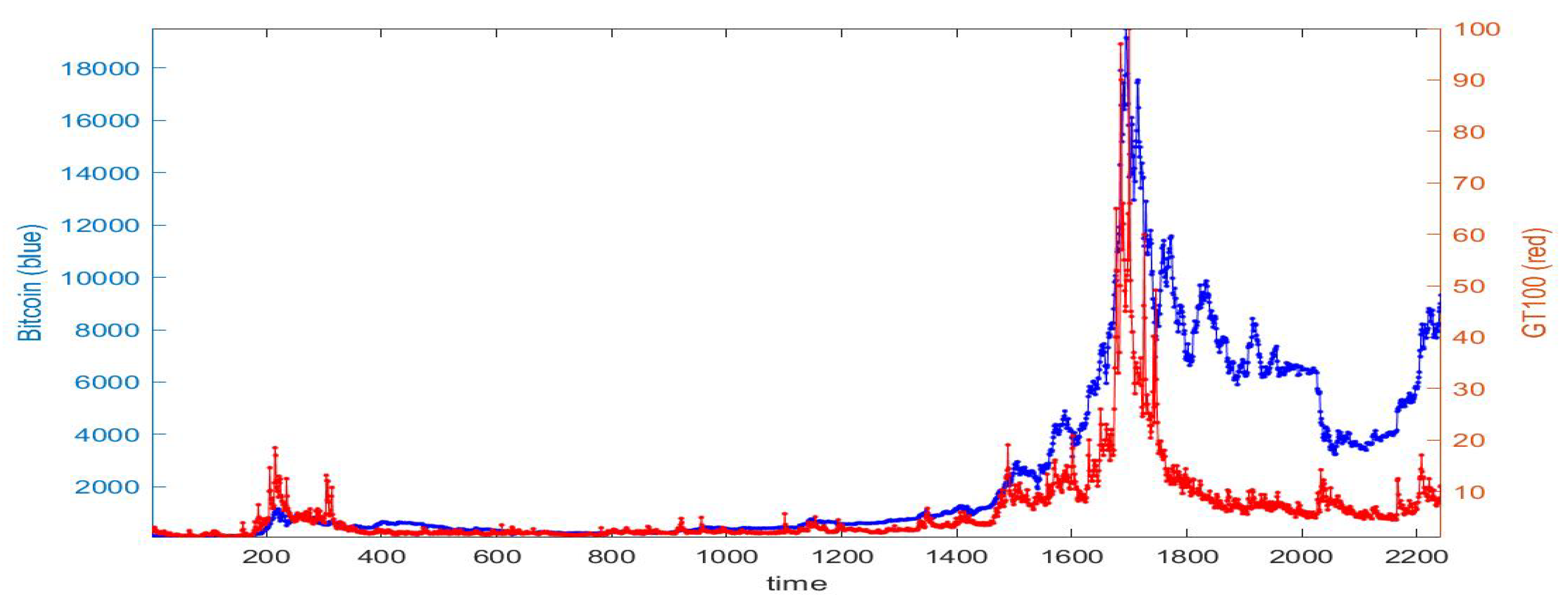
Bitcoin was released at the beginning of 2009 as a digital currency in the market; it remained under $0.20 for three years and it began to increase during the first quarter of 2013. By the end of 2017, Bitcoin was valued at nearly $18,000 per “coin”. In 2018, the price plummeted $4000 and it grew again in 2019.

The second dataset we consider is Google Trends, the search index that measures what people are currently interested in and curious about. In particular, we consider Google Trends with value 100 out of 100 meaning that trend (word Bitcoin) is on its peak in the considered time period.

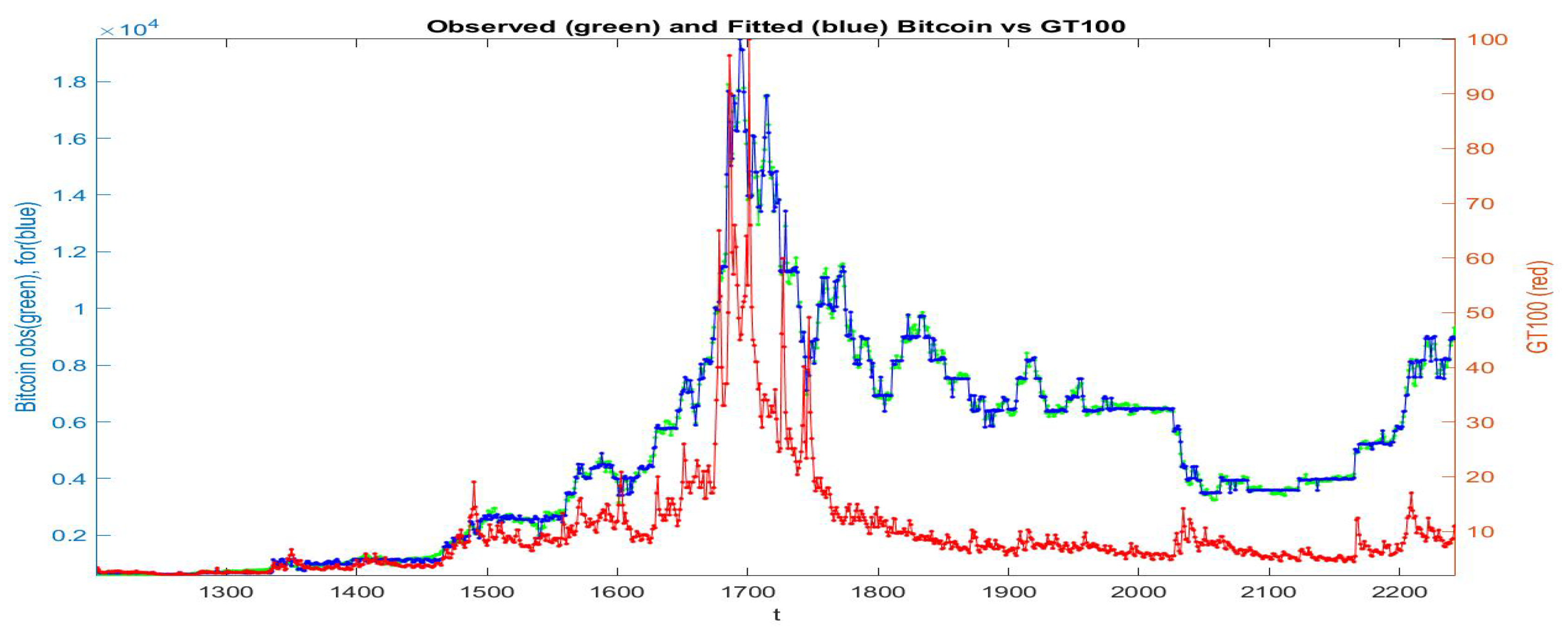
Here, we work on two daily time series, as in Figure 1, from April 2013 to June 2019: Bitcoin prices (from www.blockchain.info) and Google Trends (from https://trends.google.com). The label time in the figures refers to daily observation number (t = 1 corresponds to the first observation considered); the labels Bitcoin and GT100 denote the arrays with the data.

Remark that the F-transform (direct and inverse) is linear with respect to the data-set, in particular it is homogeneous and scale invariant: we can normalize the two time series and the direct F-transform components (or the iF-transform function) are multiplied by the same factor. In this way, we can compare the F-transform results for the two series in terms of the obtained smoothing effect and by visualizing the scatter-plots of the of each series and the obtained iF-transform reconstructions.

The degree of smoothness of a given time series $f_t$, $t=1,2, \dots , M$ is measured in terms of its (average) absolute variation, given by

$$V\left(f\right)={\displaystyle \frac{{\displaystyle \sum _{t=1}^{M-1}}|f_{t+1}-f_t|}{M-1}};$$

(32)

on the other hand, it is well known that the inverse $L_p$-norm F-transform function, for a fixed r-partition $(\mathbb{P},\mathbb{A},r)$, allows the computation of the smoothing values

$$f_t^{\left(r\right)}=\frac{1}{r}\sum _{k=2-r}^{n+r-1}{\vartheta }_k\left(t\right)A_k\left(t\right) \mathrm{for} t=1, 2, \dots , M$$

(33)

corresponding to the estimated (local) polynomials of order q, ${\vartheta }_k\left(t\right)={\theta }_{k,0}+{\theta }_{k,1}(t-x_k)+ \dots +{\theta }_{k,q}{(t-x_k)}^q$, $k=2-r, \dots , n+r-1$. The corresponding absolute variation, given by

$$V\left(f^{\left(r\right)}\right)={\displaystyle \frac{{\displaystyle \sum _{t=1}^{M-1}}|f_{t+1}^{\left(r\right)}-f_t^{\left(r\right)}|}{M-1}},$$

(34)

is in general smaller than $V\left(f\right)$; the ratio

$$L(f,f^{\left(r\right)})={\displaystyle \frac{V\left(f^{\left(r\right)}\right)}{V\left(f\right)}}$$

(35)

represents the proportion of absolute variation which remains in the smoothed time series $f^{\left(r\right)}$ with respect to the original data f, while $1-L(f,f^{\left(r\right)})$ is the amount of removed variation.

We have computed the $L_p$-norm F-transforms for different values of $p\in \left\{1,1.25,1.5,1.75,2\right\}$ and orders $q\in \left\{0,1,3\right\}$. The excellent performance of the smoothing based on F-transform are strongly confirmed for these two special time series, as summarized in

Table 1. $L_p$-norm F-transform of Bitcoin and GT100 time series For five values p and three orders $q\in \left\{0,1,3\right\}$ the table shows ratios $L(f,f^{\left(r\right)})$ with $f\in \left\{Bitcoin,GT100\right\}$.

p	q	Bitcoin	GT100
1	0	0.3526	0.1646
1	1	0.4298	0.2643
1	3	0.5813	0.4922
1.25	0	0.3493	0.1628
1.25	1	0.4315	0.2677
1.25	3	0.5693	0.4813
1.5	0	0.3465	0.1649
1.5	1	0.4282	0.2702
1.5	3	0.5558	0.4785
1.75	0	0.3448	0.1777
1.75	1	0.4250	0.2783
1.75	3	0.5483	0.4798
2	0	0.3428	0.1715
2	1	0.4221	0.2859
2	3	0.5432	0.4815

and

Table 2. Approximation indices for $L_p$-norm F-transform of Bitcoin and GT100 For five values $p\in \left\{1,1.25,1.5,1.75,2\right\}$ and three orders $q\in \left\{0,1,3\right\}$ the table shows indices $MSE$, $\%MAE$, and Kendall $\tau$ correlation for the pairs $(f,f^{\left(r\right)})$ with $f\in \left\{Bitcoin,GT100\right\}$.

			Bitcoin			GT100
p	q	$MSE$	$\%MAE$	$\tau$	$MSE$	$\%MAE$	$\tau$
1	0	363.98	2.5173	0.9766	2.7670	7.8219	0.8897
1	1	201.66	2.0152	0.9815	1.8610	6.7139	0.9049
1	3	148.75	1.4739	0.9860	1.5614	4.8293	0.9331
1.25	0	219.72	2.5171	0.9768	2.3939	7.9307	0.8911
1.25	1	191.58	2.0315	0.9817	1.8211	6.8342	0.9074
1.25	3	139.34	1.4874	0.9863	1.4556	4.9210	0.9345
1.5	0	217.61	2.5641	0.9765	2.3339	8.1374	0.8910
1.5	1	190.20	2.0805	0.9814	1.8027	7.0240	0.9068
1.5	3	137.72	1.5284	0.9861	1.4169	5.1172	0.9331
1.75	0	217.79	2.6232	0.9762	2.3020	8.3932	0.8896
1.75	1	191.26	2.1298	0.9810	1.7920	7.2505	0.9057
1.75	3	137.75	1.5734	0.9858	1.4031	5.3430	0.9311
2	0	219.41	2.6859	0.9757	2.2855	8.6858	0.8877
2	1	192.74	2.1778	0.9708	1.7964	7.4879	0.9038
2	3	138.46	1.6155	0.9856	1.4040	5.5762	0.9289

.

All computations are performed with a 1-partition ($r=1$), a decomposition $\mathbb{P}$ of $[1,M]$ into $n=326$ equispaced nodes and basic functions obtained from $L\left(\tau \right)={\displaystyle \frac{{\tau }^2}{1-2\tau (1-\tau )}}$, $\tau \in [0,1]$. For both series, covering the same time period, we have $M=2276$ so that each subinterval $\left[x_k,x_{k+1}\right]$, $k=1, \dots , n-1$ of $\mathbb{P}$ has exactly 8 observations (13 observations internal to intervals $\left[x_{k-1},x_{k+1}\right]$, $k=2, \dots , n-1$ on which basic function $A_k$ is non-zero); remark that the two series are observed all days of the week, including holidays, so that all internal nodes $x_k$ of $\mathbb{P}$ correspond to the same day in the week.

For the results of Table 1, the observed values are normalized in the range $\left[0,1000\right]$; on this common range, the computed absolute variations are $V\left(Bitcoin\right)=4.6354$ and $V\left(GT100\right)=6.9986$ and Bitcoin is $66.23\%$ less fluctuating (on average) than GT100. For all values of p, the reduction in total variation expressed by the ratios $L(f,f^{\left(r\right)})$, for both series, is more depending on the order q than on the used norm $L_p$; this is not surprising, because increasing the degree of local polynomials will reduce the average fitting errors but increase their variation.

In Table 2 the smoothing and fitting of the time series by $L_p$-norm F-transforms are compared in terms of three well-known indices: the mean square error MSE, the mean absolute percentage error $\%MAE$ and the Kendall $\tau$ rank correlation.

Here the series are not normalized (in particular, the value of index $MSE$ depends on the scale of the series). In all cases, the F-transform fitting for Bitcoin series has significantly smaller errors than for GT100, as demonstrated by indices $\%MAE$ and $\tau$ (the Kendall $\tau$ is always significantly positive with p-value less than ${10}^{-8}$).

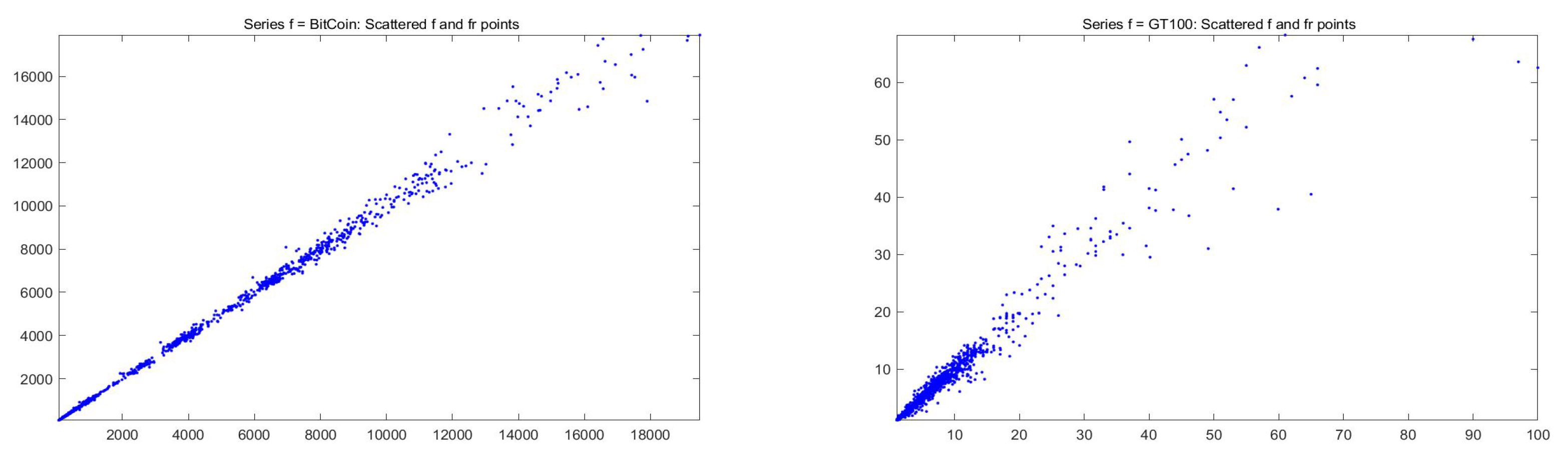
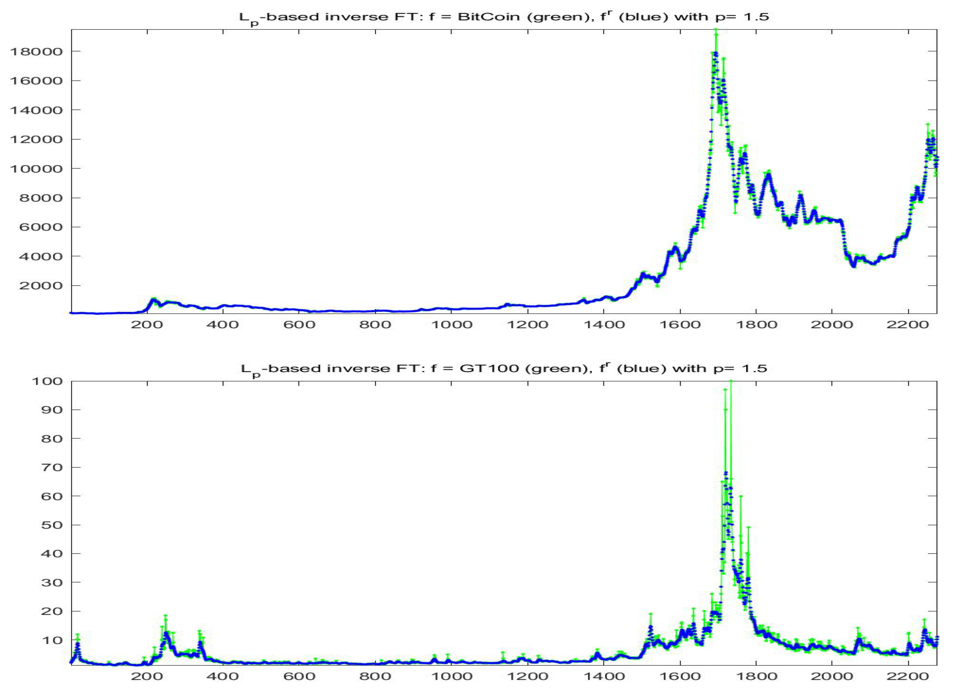
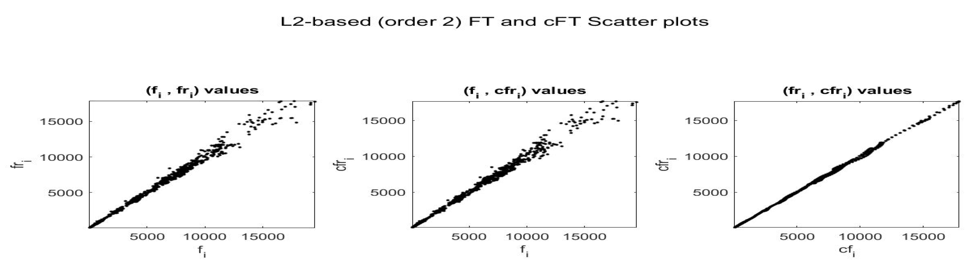
For the fitting F-transform functions obtained by $L_p$-norm with $p=1.5$ and $q=0$, the scatter-plots of time series $(f_t,f_t^r)$ are pictured in Figure 2; Figure 3 plots $f_t$ and $f_t^r$ with respect to time. Remark that peaks in the series tend always to be smoothed, as a characteristics of the smoothing effect produced by F-transform.

Assuming a bi-directional dependence between $GT100$ and $Bitcoin$ time series, empirically demonstrated, e.g., in [27], and focusing on the impact of $GT100$ on $Bitcoin$, we want now to investigate the form of dependence by use of expectile (fuzzy-valued) F-transform; in particular, we see that while the fitting of iF-transform obtained on the totality of observed values $(BitCoi{n}_t,GT{100}_t)$ presents a high dispersion, a very big improvement in the fitting quality is obtained if F-transform is applied to clustered subsets of observed data. A relatively small number of clusters (from 20 to 24) in sufficient to obtain a fitting with correlation coefficient greater than $0.99$.

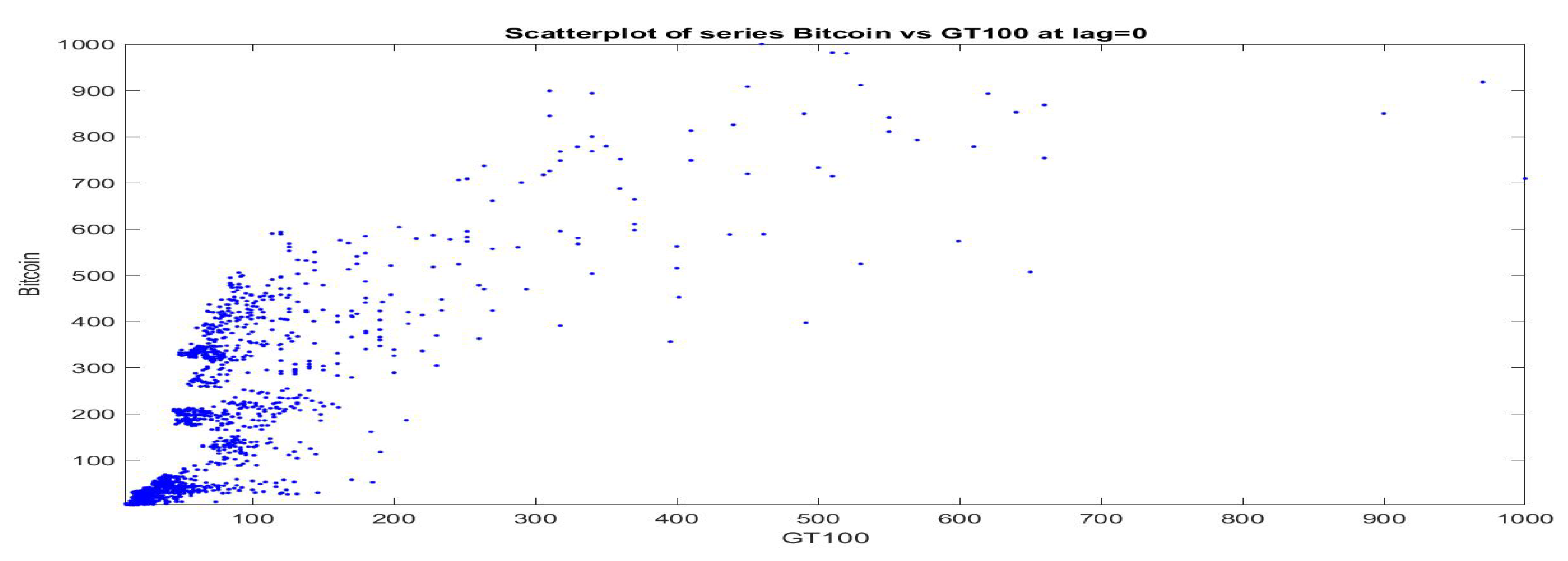
First of all, a scatter plot of the pairs is pictured in Figure 4 (the two time series are normalized in the range $[0,1000]$ and GT100 appears in horizontal axis); observations in our data-set cover the cited time period 2013–2019, are concentrated on the bottom-left part of the positive quadrant and have rare points with big values in both series. At a first look, no evident functional relationships emerge from the data; they simply show a tendency to be co-monotonic, but the points are very sparse.

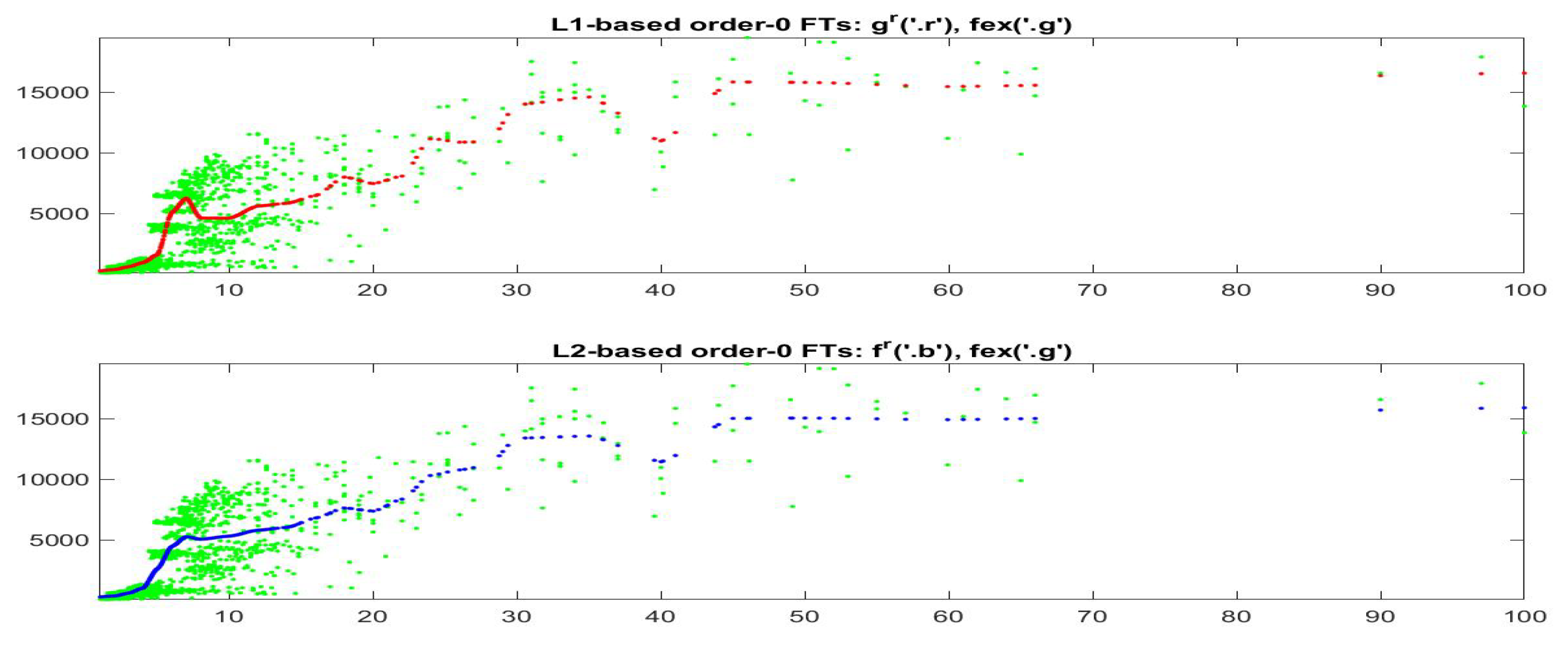
For a deeper analysis, we propose a model based on F-transform, relating the pairs of data $(GT{100}_t,BitCoi{n}_t)$. F-transform is thus used to model BitCoin as a function of GT100. The $L_1$-norm and $L_2$-norm-based inverse iF-transforms of the data-set $(GT{100}_t,BitCoi{n}_t),t=1,2, \dots , M$ are computed; taking into account the sparsity of the values $GT{100}_t$ (in particular above the threshold 40), we use a non-uniform 1-partition $(\mathbb{P},\mathbb{A})$ of the range $[0,100]$ of the observed $GT{100}_t$, namely the set of 25 nodes $\left\{0,2,3,4,5,6,7,8,10,12,14,16,18,20,22,24,26,28,30,35,40,45,50,60,100\right\}$, as pictured in Figure 5. The two curves give the predominant relationship between $BitCoin$ and $GT100$. It is evident that both iF-transforms of $BitCoi{n}_t$ are not increasing on the whole range of $GT100$ (in particular, they decrease when GT100 is around 7–8, around 20 and 40). On the other hand, observing the dispersion of points in Figure 4, both iF-transforms are not good fitting of the complete data-set and it appears that the points can be “clustered”, e.g., for different levels of Bitcoin prices, and better sub-fittings can be attempted.

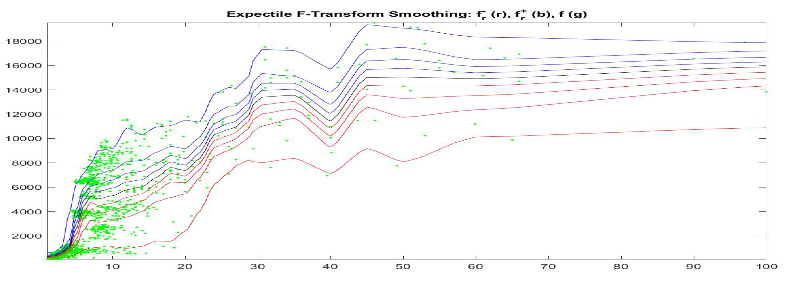
This can be better analyzed by applying the quantile and the expectile F-transforms to our data-set $(GT{100}_t,BitCoi{n}_t)$, pictured in Figure 6, which shows the fuzzy-valued expectile F-transform of Bitcoin as a function of GT100 for five different $\alpha$-cuts corresponding to $\alpha \in \{0.01,0.25,0.5,0.75,1\}$ (i.e., ten values $\omega \in \{\frac{\alpha }{2},1-\frac{\alpha }{2};all$ $\alpha \}$ for the asymmetry expectile parameter $\omega$).

We see that corresponding to different values of $\alpha$, i.e., corresponding to subintervals in the range of Bitcoin prices, the relationship between our time series changes significantly.

This suggests that possibly, the clustering of the data into subsets may significantly improve the quality of fitting.

Clearly, there are several procedures and criteria to cluster the observed data $(GT{100}_t,BitCoi{n}_t)$; we use the well-known k-means method and the number of clusters is selected according to the silhouette measures available in MATLAB R2018b. We have performed three types of clusters, the first on the basis of variable $BitCoin$, the second using the pair $(BitCoin,GT100)$ and the third using observations $(BitCoin,GT100,\Delta BitCoin,\Delta GT100)$ where $\Delta$ is the first difference operator $\Delta f_t=f_t-f_{t-1}$. The clustering measure is the standard Euclidean distance.

Let $nCl$ denote the number of clusters and let $j=1,2, \dots , nCl$ be the labels of cluster $S_j$. Each observation $(BitCoi{n}_t,GT{100}_t)$ is assigned to cluster $S_{c\left(t\right)}$, i.e., the observation t is assigned to cluster labelled $c\left(t\right)\in \left\{1,2, \dots , nCl\right\}$.

For a given clustering, identified by clusters $S_1,S_2, \dots , S_{nCl}$, the $L_2$-norm-based F-transform is applied (independently) on each subset of data, for $j=1,2, \dots , nCl$,

$$S_j=\left\{(BitCoi{n}_t,GT{100}_t)|c\left(t\right)=j\right\}.$$

(36)

Finally, for the observations of each cluster, the inverse iF-transform is computed and the fitted values, for each cluster, are obtained and recomposed to obtain the fitted values for the whole dataset.

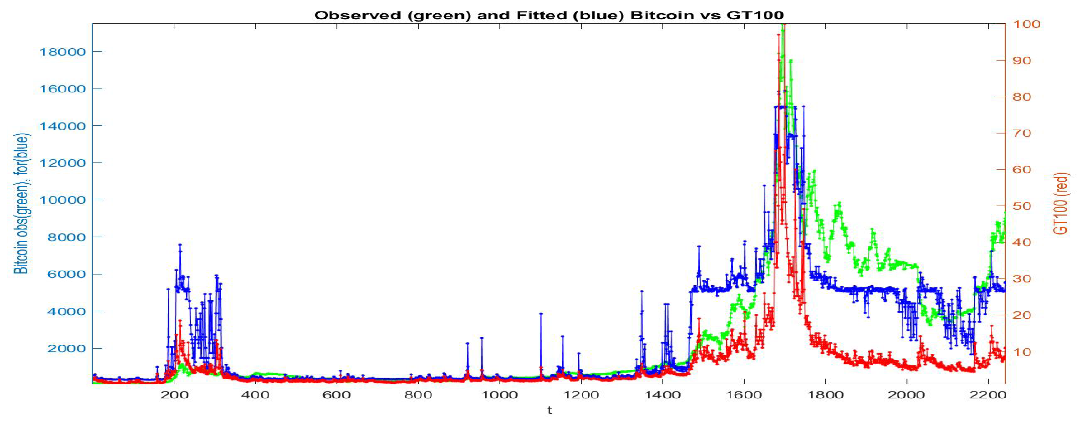
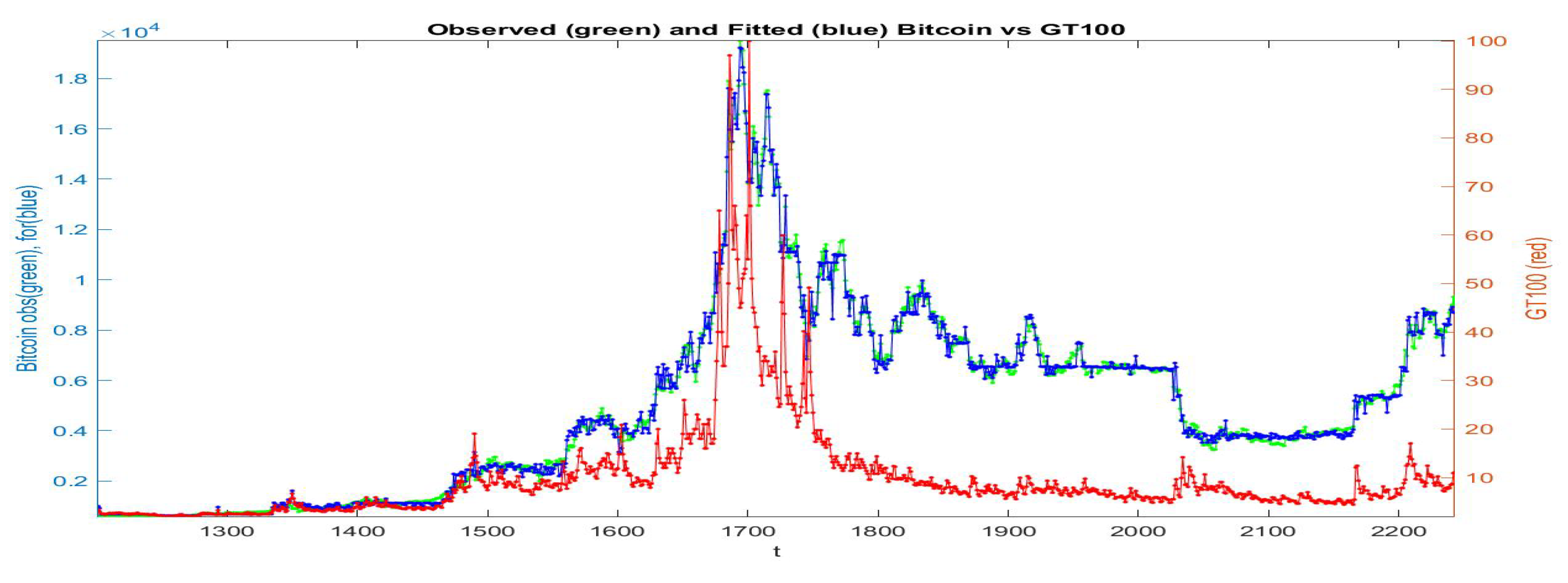
If all the data are collected in a unique cluster and the F-transform is applied to the whole data-set, we obtain the fitted $Bitcoin$ series pictured in Figure 7: the green points give the observed $BitCoi{n}_t$, the red points are the $GT{100}_t$ series and in blue is the fitting of $BitCoi{n}_t$. We see that the fitting preserves the qualitative (gross) form of the observed Bitcoin prices, but in several portions of time period the fitting is not good.

Significant improvements are obtained by adopting the three described pre-clustering, denoted respectively by labels A, B and C.

The computations are performed on the second half portion of the time period, starting with observation time $t_{1121}$; the first part is less interesting because, from observation $t_{350}$ to $t_{1220}$ both time series have small variations and relatively flat curves. Without performing pre-clustering, the $L_2$-norm F-transform reconstruction (of order 1) of $BitCoin$ in terms of $GT100$ has Kendall rank correlation $\tau =0.6049$ and Spearman correlation $\rho =0.7830$. We will compare $\tau$ and $\rho$ indices as preliminary evaluation of the effect of pre-clustering on the fitting quality.

Clustering A. Clusters are based on variable $BitCoin$: the number of clusters is $nCl=20$. The $L_2$-norm F-transform reconstruction (of order 1) of $BitCoin$ in terms of $GT100$ with pre-clustering A has much higher Kendall rank correlation $\tau =0.9457$ and Spearman correlation $\rho =0.9956$.

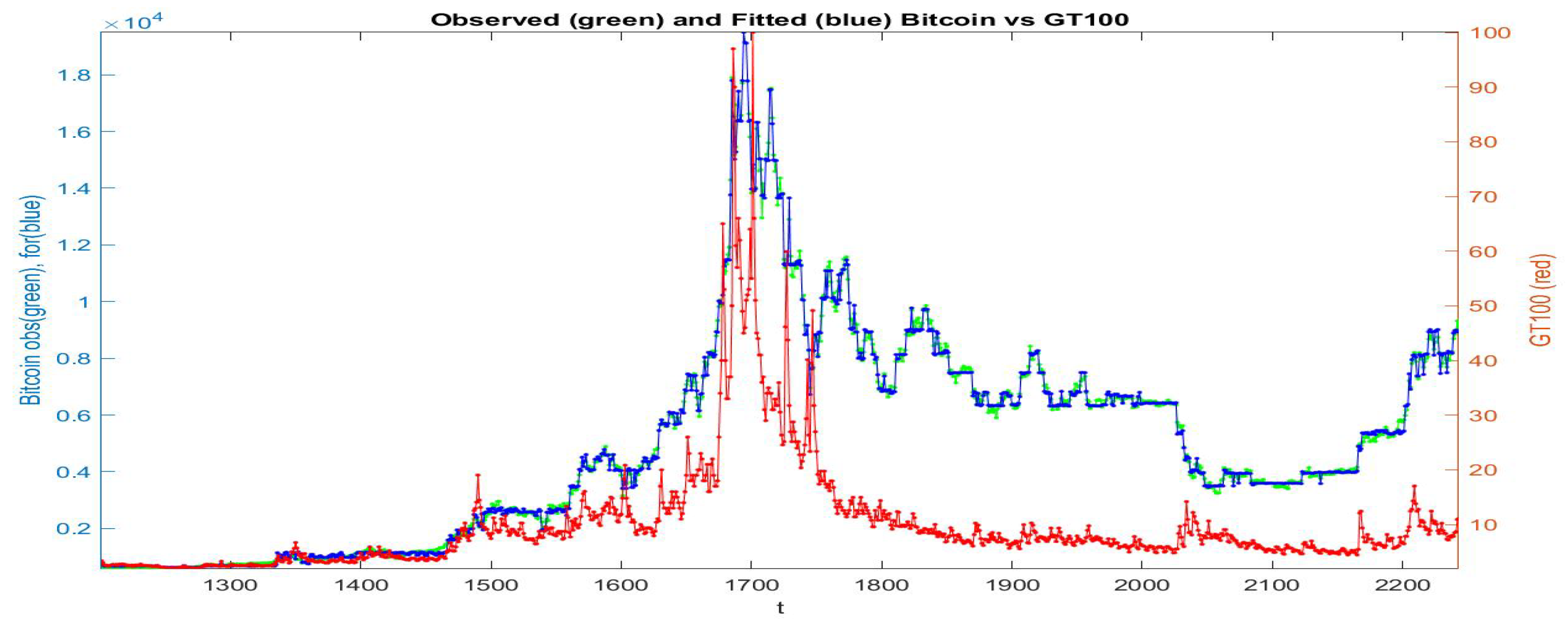
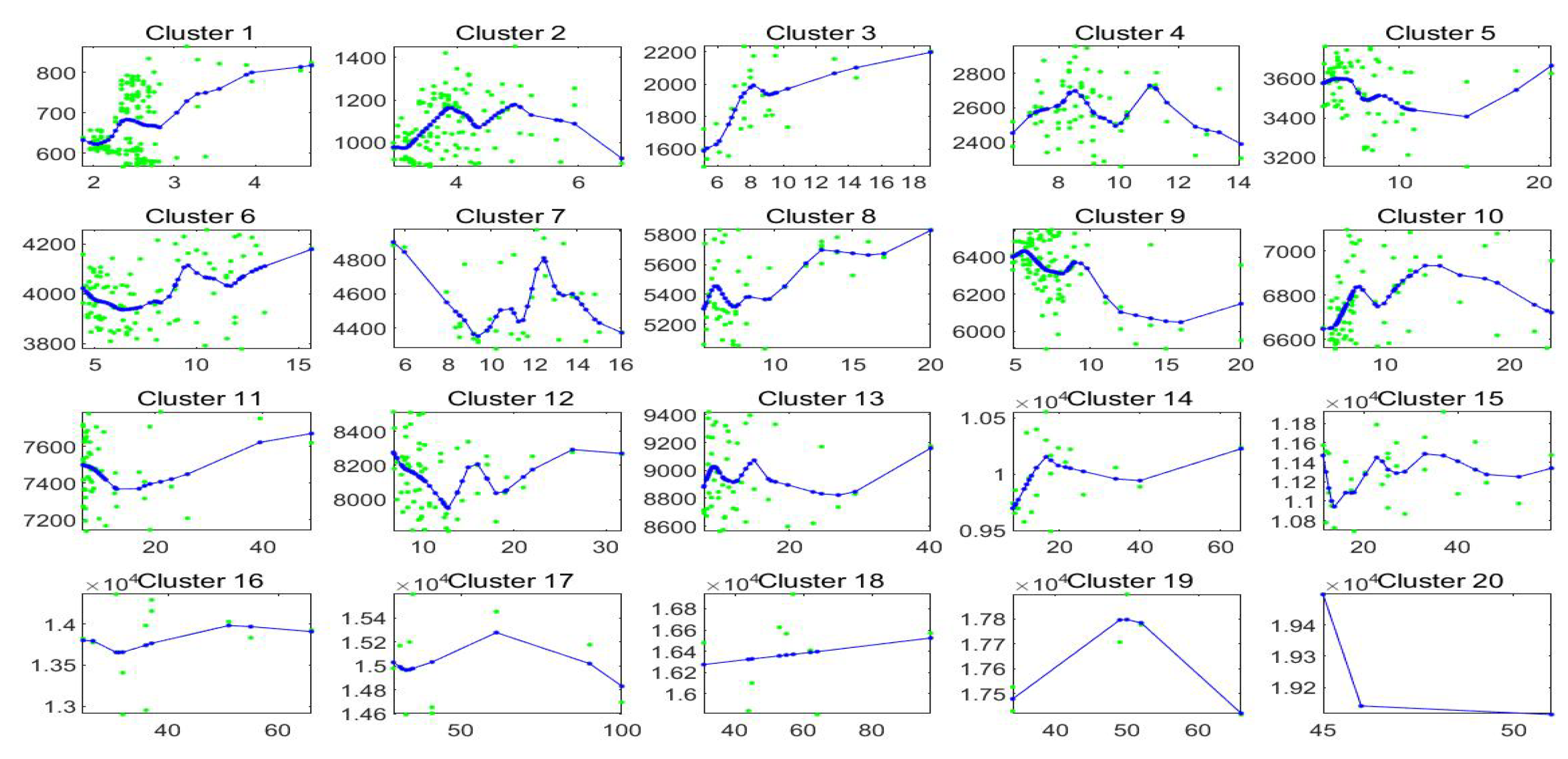
In Figure 8 we plot the observed and fitted Bitcoin series for the second half of observations, with evidence that clustering A allows a much better fitting. The 20 clusters are pictured and expanded in Figure 9 where also the sub-fittings are visible.

Clustering B. Clusters are based on both variables $(BitCoin,GT100)$: the number of clusters is $nCl=21$. The $L_2$-norm F-transform reconstruction (of order 1) of $BitCoin$ in terms of $GT100$ with pre-clustering B has high Kendall correlation $\tau =0.9447$ and Spearman correlation $\rho =0.9954$, similar to clustering A.

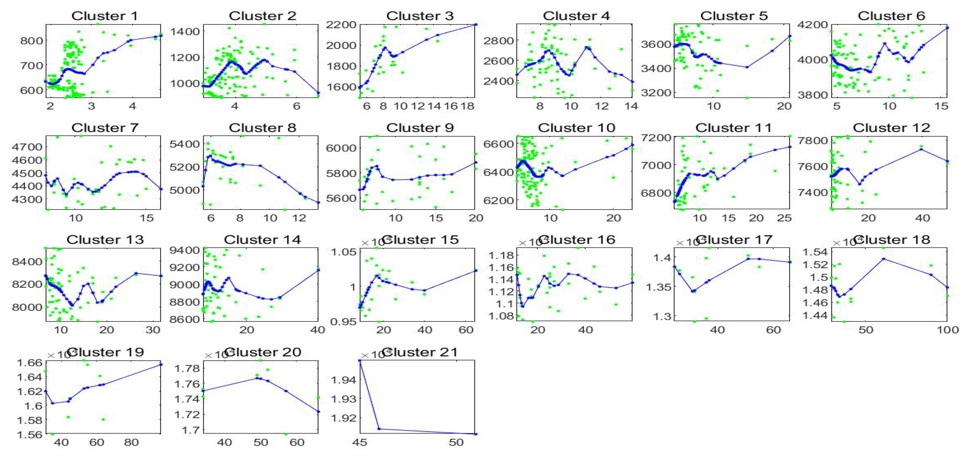
In Figure 10 we plot the observed and fitted Bitcoin series for the second half of observations, with evidence that clustering B allows a good fitting. The 21 clusters are pictured and expanded in Figure 11 where also the sub-fittings are visible.

Clustering C. Clusters are based on variables $(BitCoin,GT100,\Delta BitCoin,\Delta GT100)$; the number of clusters is $nCl=24$. The $L_2$-norm F-transform reconstruction (of order 1) of $BitCoin$ in terms of $GT100$ with this pre-clustering has high Kendall correlation $\tau =0.9183$ and Spearman correlation $\rho =0.9905$, similar but not better than pre-clustering A and B.

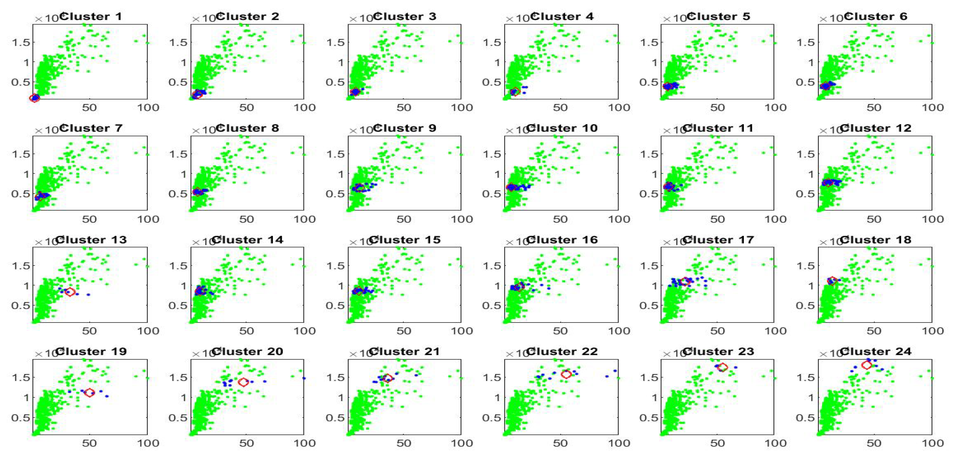
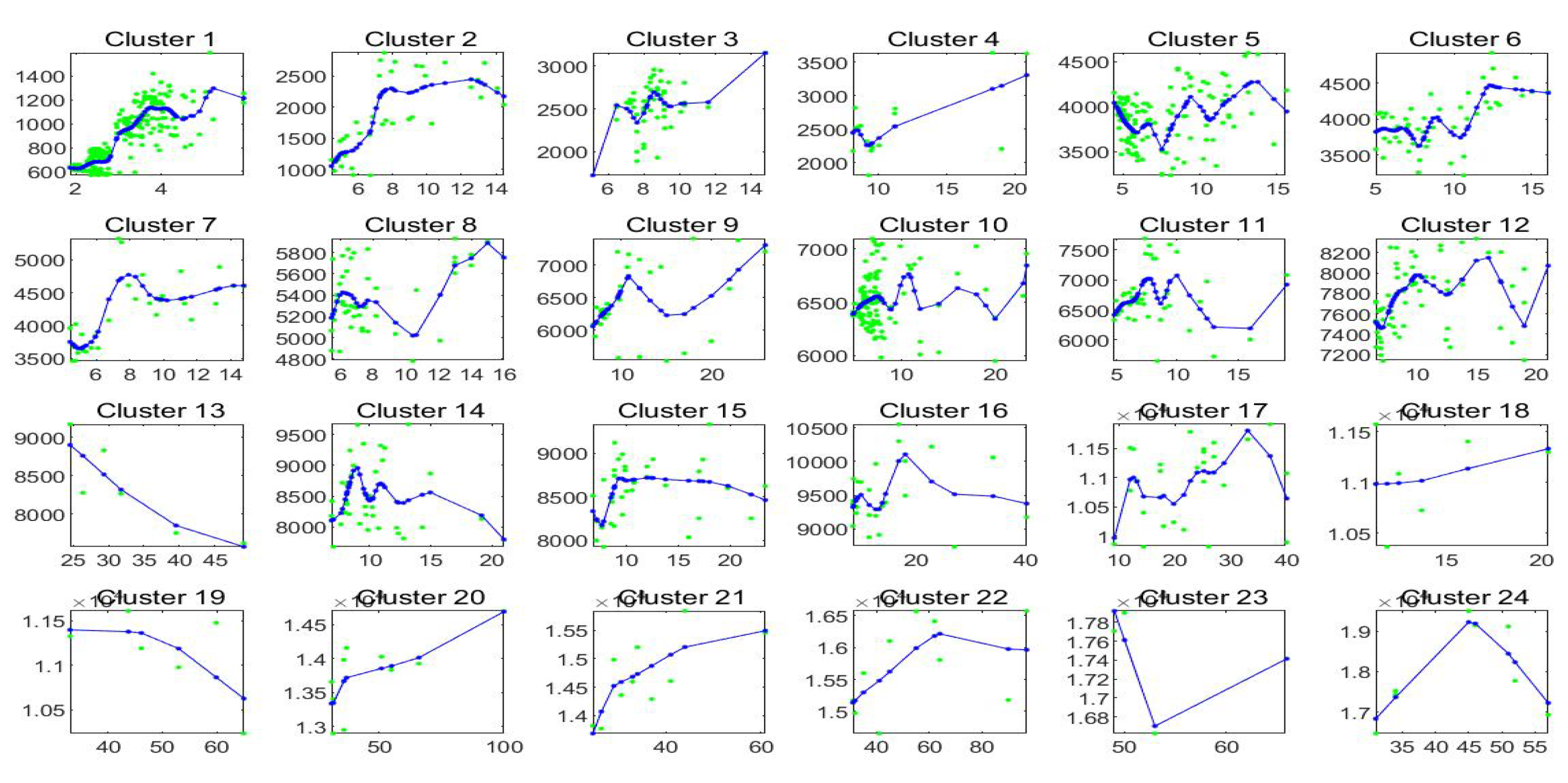
In Figure 12 we plot the observed and fitted Bitcoin series for the second half of observations, with evidence that also clustering C allows a good fitting. The 24 clusters are pictured (blue colours) in Figure 13 and expanded in Figure 14 where also the sub-fittings are pictured.

The overall result is that pre-clustering of the data, even based on very simple clustering strategies and a relatively small number of clusters (from 20 to 24) significantly improves the fitting ability of F-transform.

It is also interesting to see that the form of relationships between $BitCoin$ and $GT100$ is very different for each cluster; this has important consequences on the analysis and modeling of Bitcoin time series as, in particular, it follows different paths in various sub-periods of time and in cases of rare values of the data (e.g., big values and/or big absolute changes).

4. Stylized Facts of Bitcoin Prices Identified by F-Transform Components

The empirical identification of stylized facts, emerging from the analysis of financial time series, is a common tool in data-based approaches to time series modeling (see [49]) and is consolidated by availability of large data-sets and by application of computer-intensive efficient methods for analyzing their properties. In this section, we will analyze the local F-transform components, in particular the form of polynomials ${\phi }_k$ of $L_2$-norm F-transform, of orders $q=1$ and $q=2$ described in Section 2.1, applied to the Bitcoin time series.

We have selected the number m of daily observations such that $m-1$ is a multiple of 7 ($BitCoin$ and $GT100$ are observed all the days in the year): in this way, the available data are $m=2276$.

Consider an r-partition $(\mathbb{P},\mathbb{A},r)$ with nodes $x_k,k=1,2, \dots , n$; denoting the time points of observations simply by $t=1,2, \dots , m$ (or $t_j=j$ for $j=1, \dots , m$) we consider two uniform $(\mathbb{P},\mathbb{A},r)$:

($P_a$)—a dense partition with $n=m$ and $x_k=k$ (i.e., each observation is a node) and the bandwidth r is chosen such that each open interval $I_k^{\left(r\right)}=[x_{k-r},x_{k+r}]$ contains (internally) a prescribed sufficient number of data. E.g., with $r=4$ each $I_k^{\left(r\right)}$ contains all data of the week centred at $x_k$; with $r=7$, $I_k^{\left(r\right)}$ contains the two weeks ending and starting with $x_k$.

($P_b$)—a sparse partition with $n=326$ and $x_k=1+7(k-1)$ (i.e., there is a node every 7 observations) and the bandwidth $r=3$ is chosen. The (direct) F-transform components will span 21 observed values on each side (left or right) of the nodes.

4.1. F-Transform Fitting with Dense r-Partition

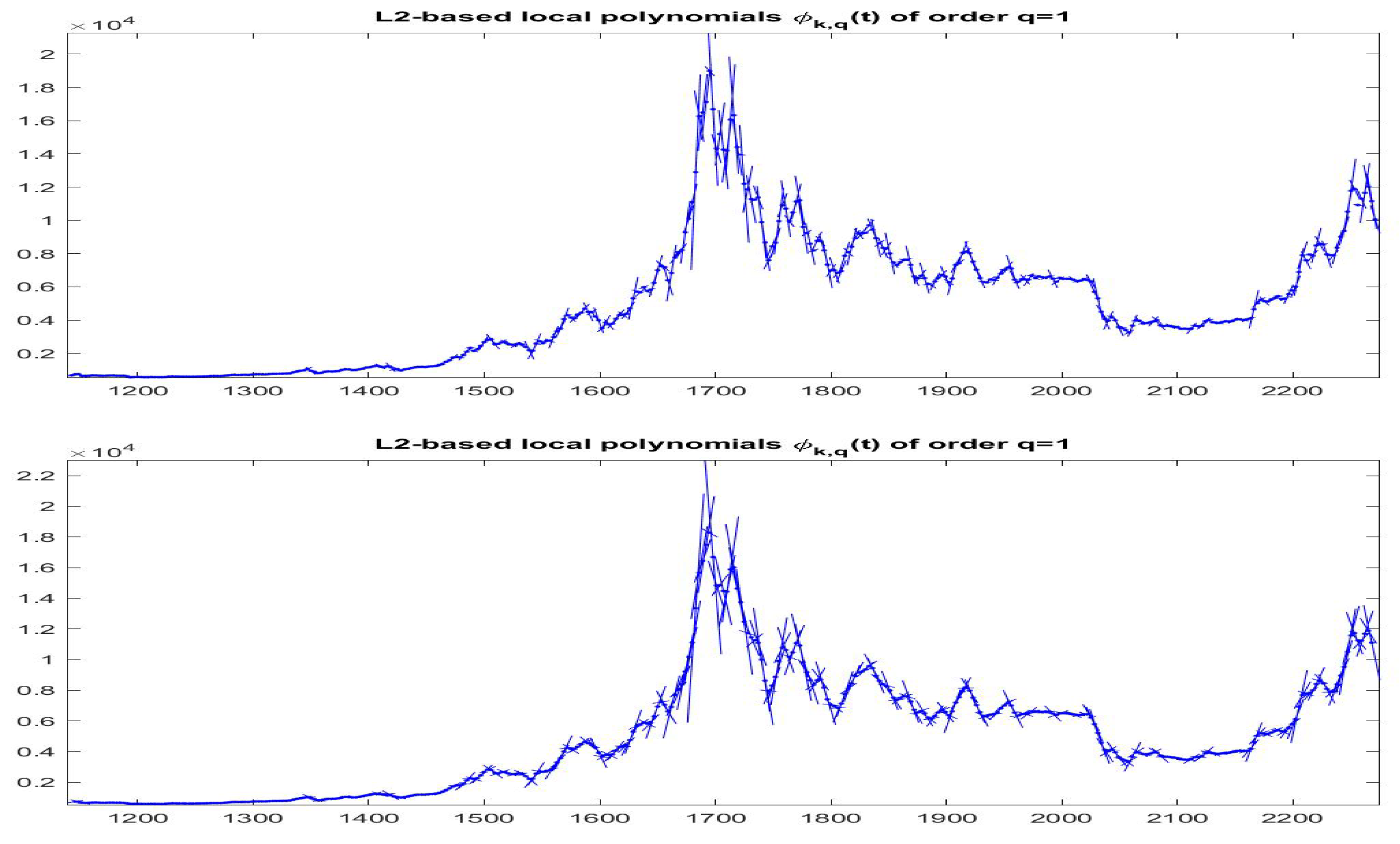
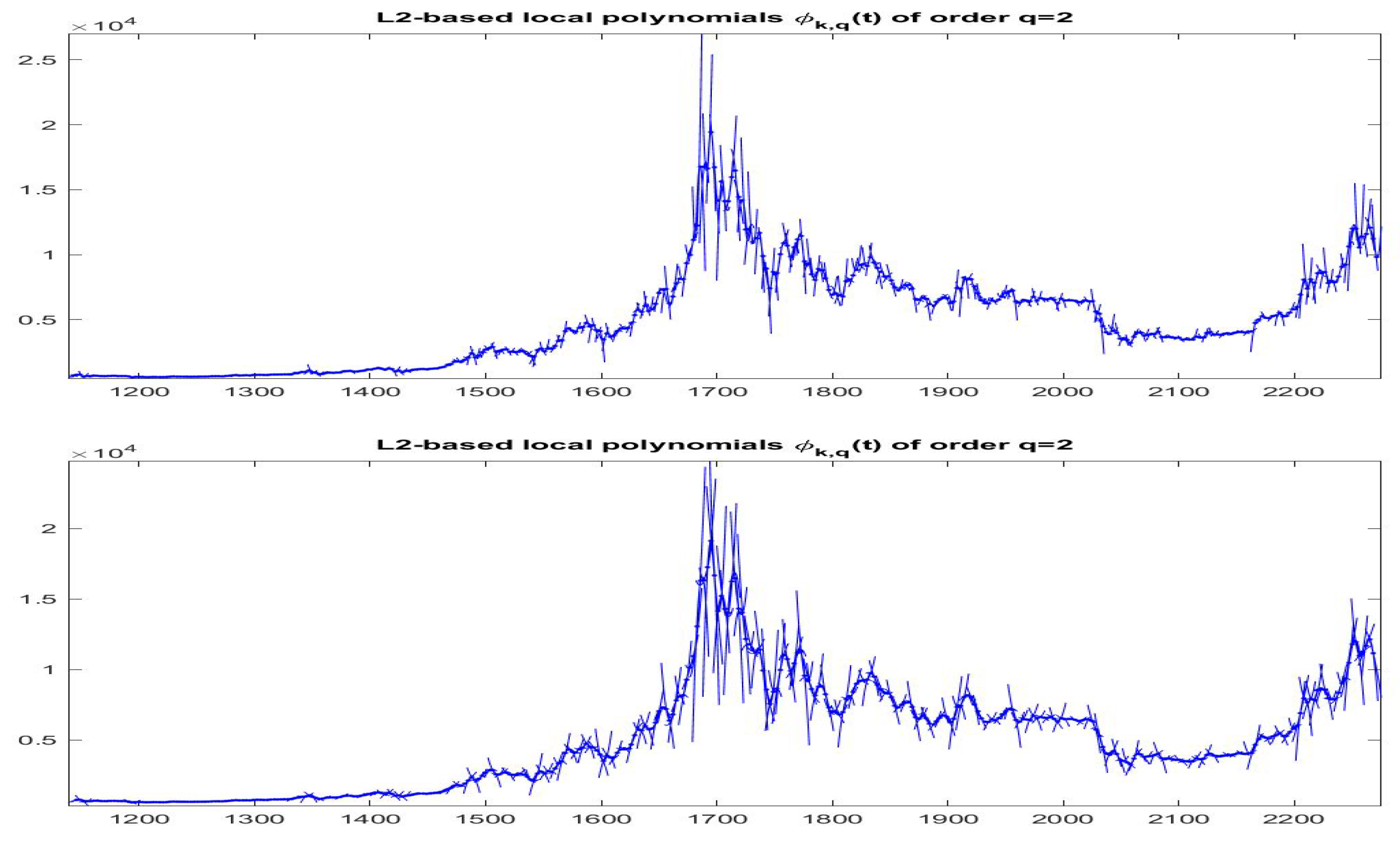
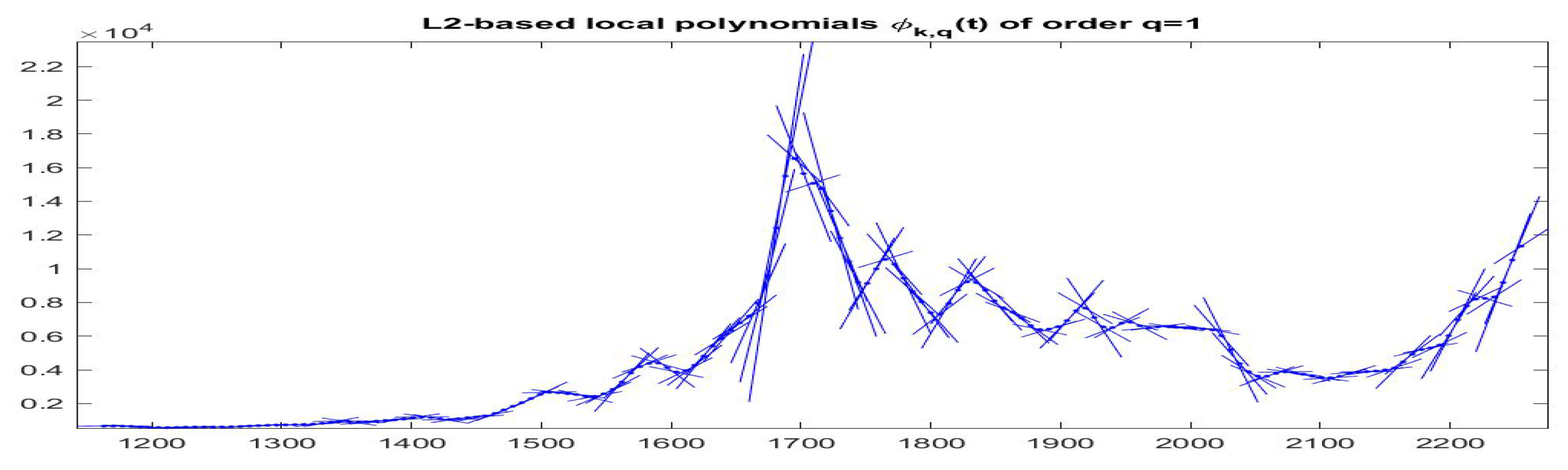
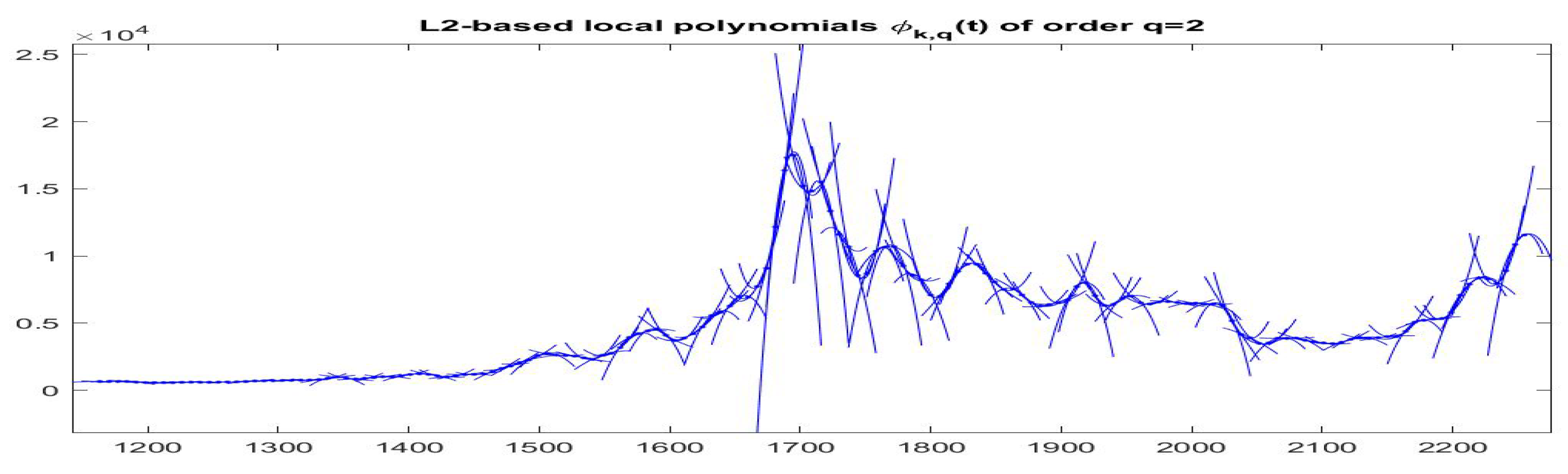
In the dense partition case, we obtain the best $L_2$-norm F-transform components ${\phi }_k\left(t\right)$ associated with all observations (indeed, $x_k=k$ corresponds to all observed times $k=1, \dots , n=m$); in this way, we are able to estimate the local trend around every observation and se can follow the time evolution of trends by plotting ${\phi }_k\left(t\right)$ around $x_k$ on subintervals $I_k^{\left(r\right)}$ (see Figure 15 and Figure 16).

On the other hand, if we translate vertically the polynomials ${\phi }_k\left(t\right)$, the polynomials ${\widehat{\phi }}_k\left(t\right)={\phi }_k\left(t\right)-{\varphi }_{k,0}$ are such that ${\widehat{\phi }}_k\left(x_k\right)=0$ for all k and, if $q>0$, we can cluster the ${\widehat{\phi }}_k$ by clustering the set of vectors $({\varphi }_{1,k}, \dots , {\varphi }_{q,k})$ of the estimated coefficients. If $q=1$ we obtain a set of lines through the origin with different slopes (in terms of a single variable ${\varphi }_{1,k}$); if $q=2$ we obtain a set of parabolic functions through the origin, in terms of two variables ${\varphi }_{1,k}$ and ${\varphi }_{2,k}$.

Using the k-means clustering method with the Euclidean distance and testing the number of clusters using the silhouette values, we have that the best number of clusters is $nCl=9$ when $q=1$ and $nCl=15$ when $q=2$.

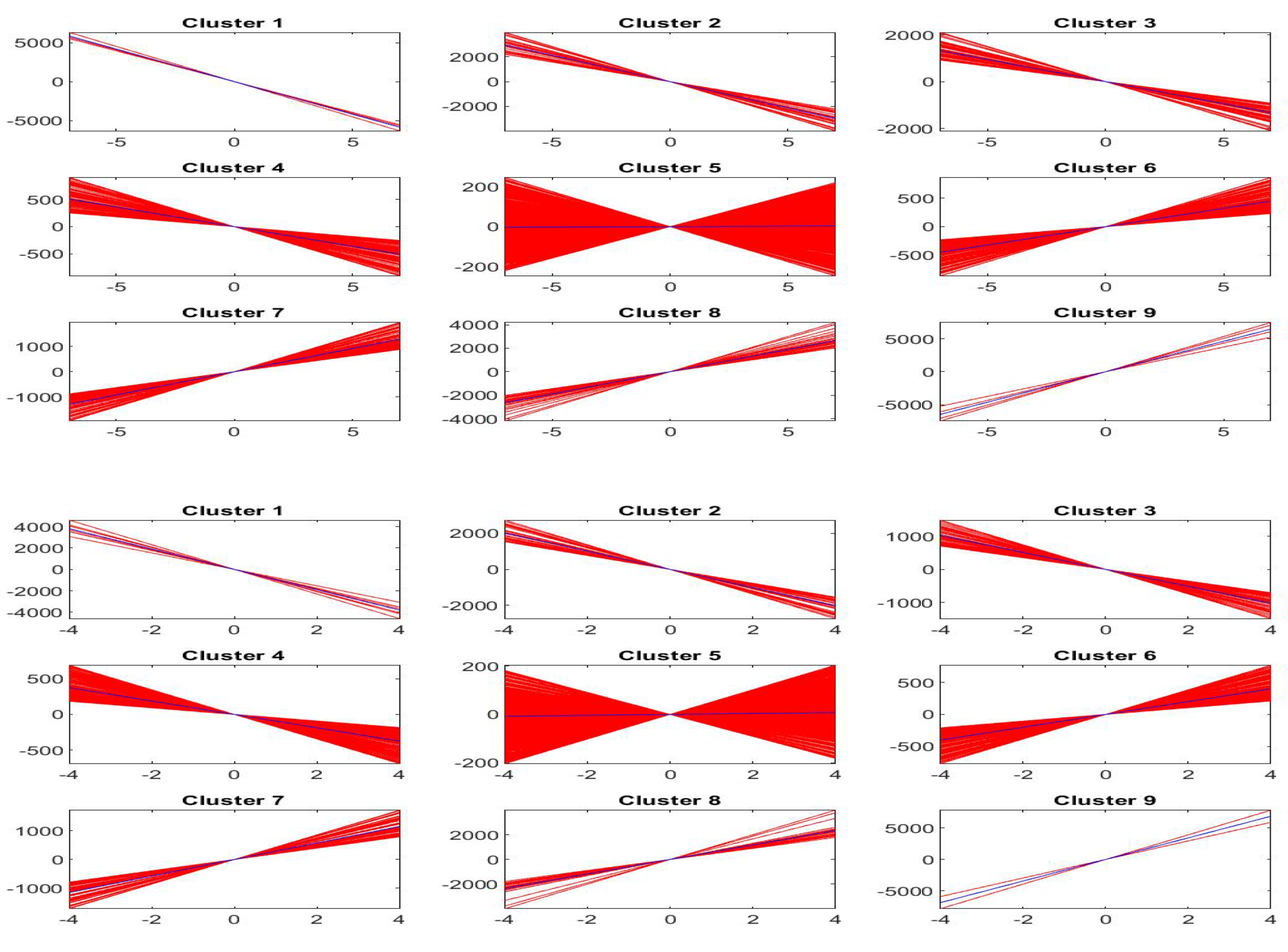
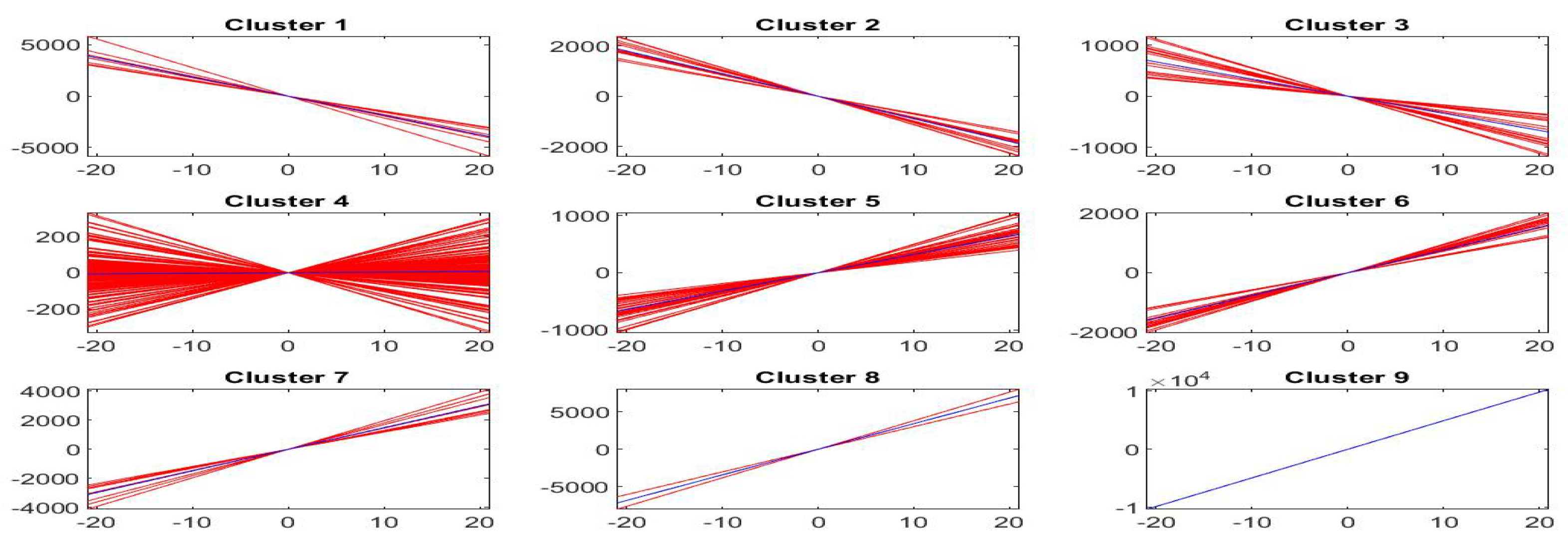
The interpretation of $nCl=9$ clusters (characterized by variable ${\varphi }_{1,k}$) is interesting, because we have a central cluster of local trends with slope around 0 and other eight clusters characterized by slopes ranging from very negative values (cluster 1) to intermediate negative values (cluster 3) up to intermediate positive (cluster 7) to very positive slopes (cluster 9).

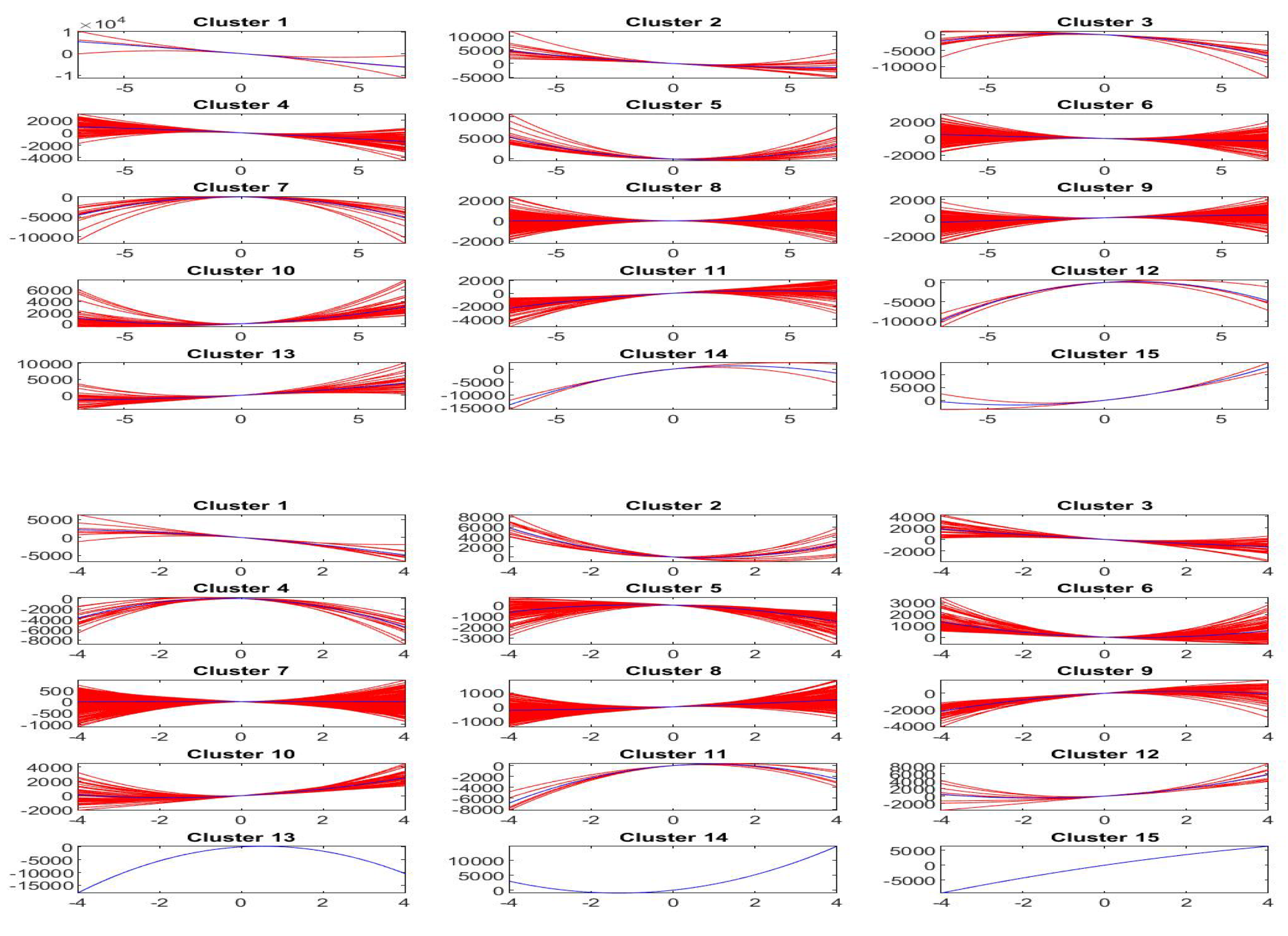
Analogous interpretation is applied to the case of $nCl=15$ clusters (and $q=2$), where again cluster 1 corresponds to the most negative slope, cluster 8 to almost zero slope and cluster 15 to the most positive slope; clearly, also the degrees of concavity and convexity (represented by the second variable ${\varphi }_{2,k}$) are taken into account in this case.

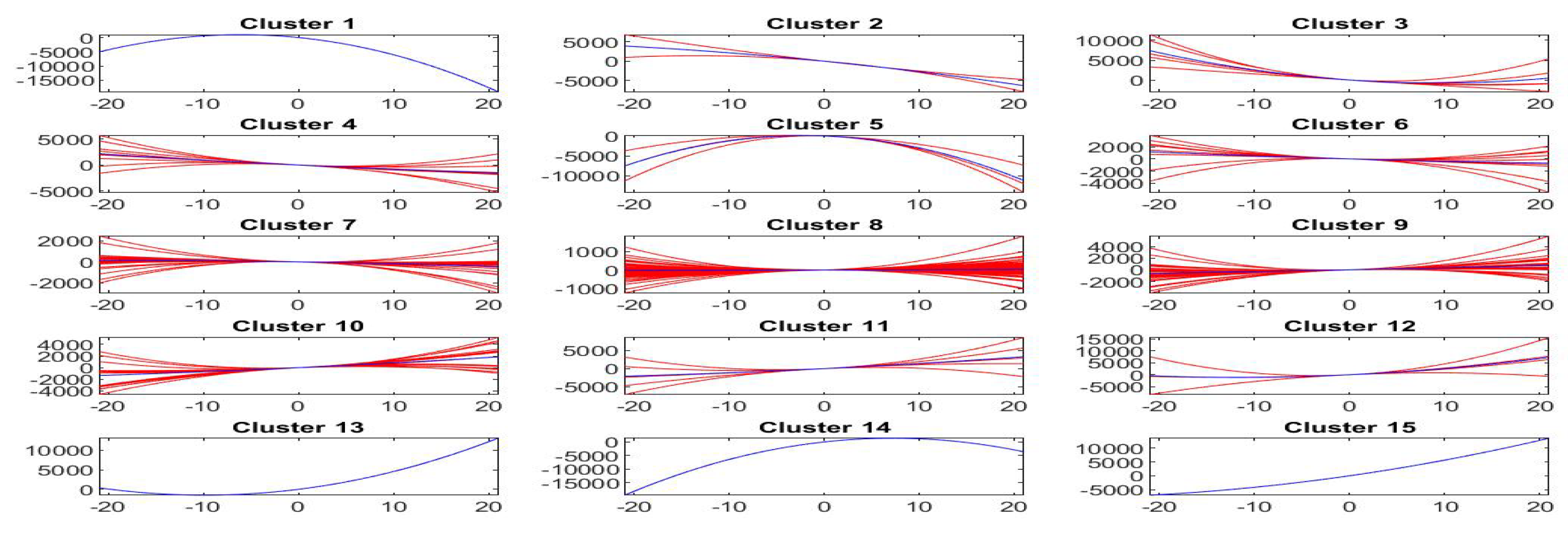
Figure 17 pictures, for each cluster $S_c^{\left(1\right)}$, $c=1,2, \dots , 9$, the first order shifted polynomials ${\widehat{\phi }}_k\left(t\right)={\varphi }_{1,k}(t-x_k)$ assigned to $S_c^{\left(1\right)}$ (red colors) and the centroid polynomial (blue color) obtained by averaging the parameters ${\varphi }_{1,k}$.

Similarly, Figure 18 pictures, for each cluster $S_c^{\left(2\right)}$, $c=1,2, \dots , 15$, the second order shifted polynomials ${\varphi }_{1,k}(t-x_k)+{\varphi }_{2,k}{(t-x_k)}^2$ assigned to $S_c^{\left(2\right)}$ (red colors) and the centroid polynomial (blue color) obtained by averaging the pairs of parameters $({\varphi }_{1,k},{\varphi }_{2,k})$.

As we have said, the $nCl$ centroid polynomials, identified by averaging the parameters of all elements assigned to each cluster $S_c^{\left(1\right)}$ or $S_c^{\left(2\right)}$, can be considered to be the stylized forms of the local trends. If we identify each estimated trend by the centroid of its cluster, we then have $nCl$ stylized forms, one for each cluster, that form the possible typical trends around the observed points of the time series.

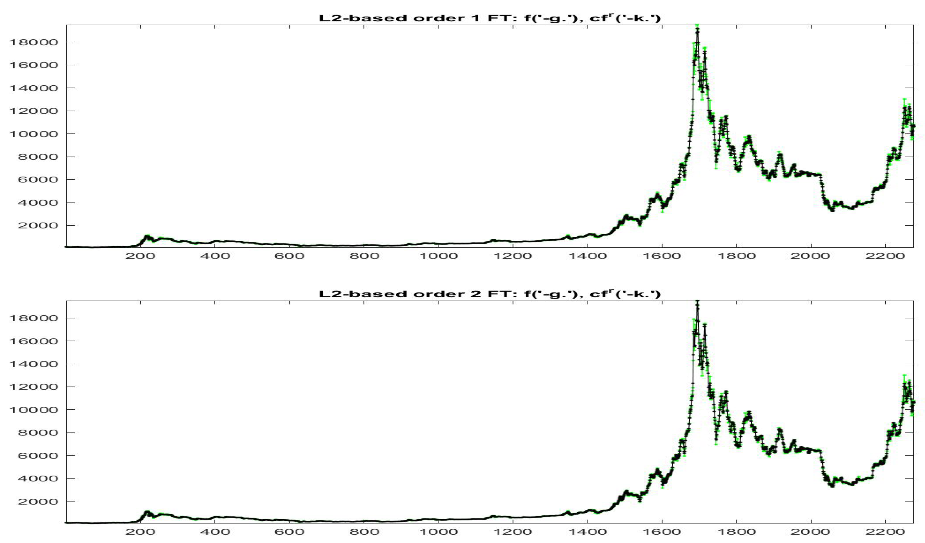
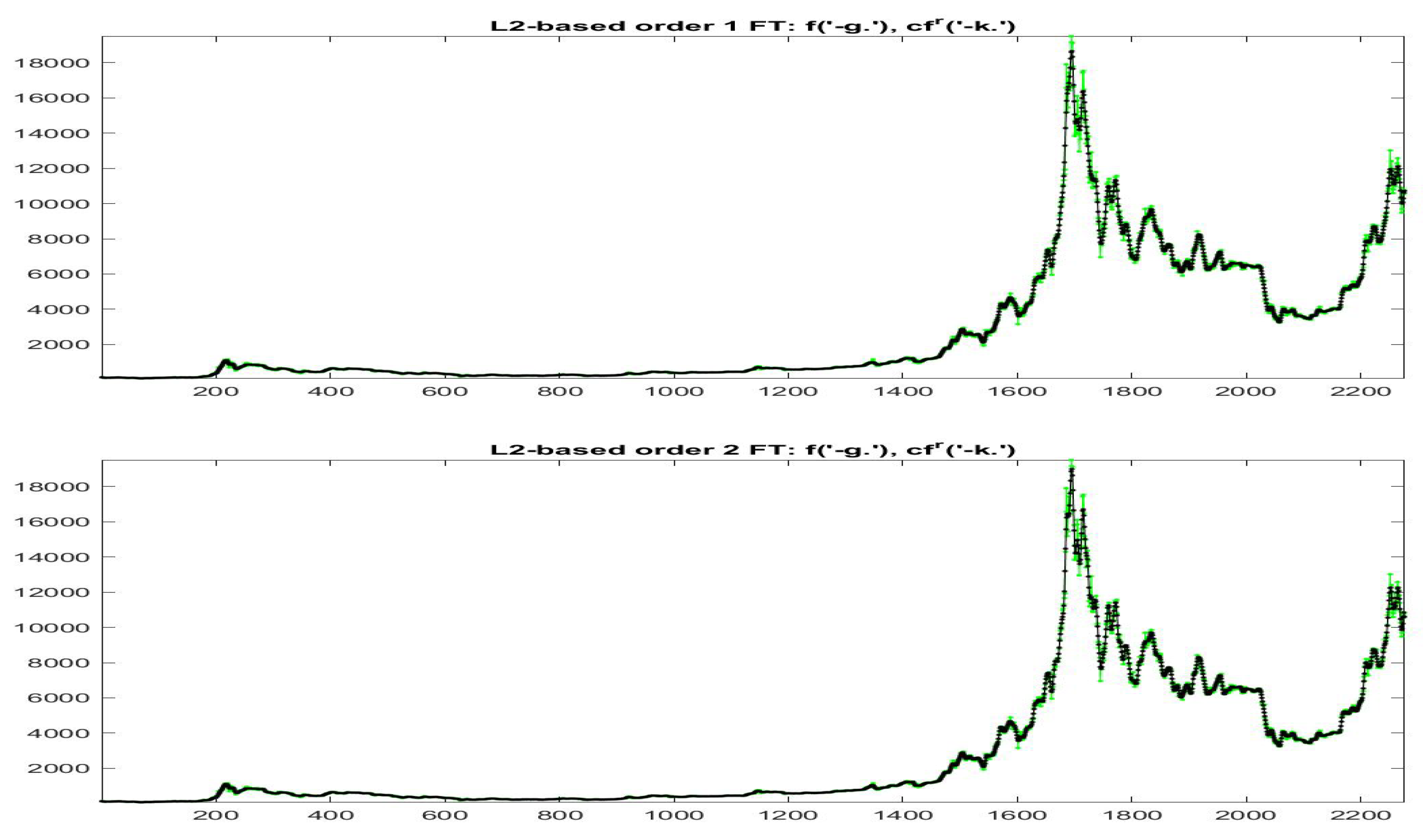
As a last step, we can produce a simple analysis of how good the stylized trends represent the effective observations: let’s denote by $f_{({\mathbb{P}}_a,\mathbb{A},r)}^q\left(t_j\right)$ the standard inverse iF-transform values at times $t_j$ obtained with estimated direct F-transform (polynomial) components ${\phi }_k\left(t\right)$, i.e.,

$$f_{({\mathbb{P}}_a,\mathbb{A},r)}^q\left(t\right)=\frac{1}{r}\sum _{k=2-r}^{n+r-1}{\phi }_k\left(t\right)A_k\left(t\right);$$

(37)

denote by $f_{c,({\mathbb{P}}_a,\mathbb{A},r)}^q\left(t_j\right)$ the analogous expression obtained by substituting each local polynomial ${\phi }_k\left(t\right)$ by ${\widehat{\phi }}_k\left(t\right)={\varphi }_{0,k}+{\widehat{\varphi }}_{1,k}(t-x_k)+ \dots +{\widehat{\varphi }}_{q,k}{(t-x_k)}^q$ (here $q=1$ or $q=2$), where the parameters ${\widehat{\varphi }}_{1,k}$ or the pairs $({\widehat{\varphi }}_{1,k},{\widehat{\varphi }}_{2,k})$ are the ones that identify the centroid of cluster containing time k, i.e., if an observation belongs to cluster $S_c$ we substitute the computed local trend with the local trend of the corresponding centroid:

$$f_{c,({\mathbb{P}}_a,\mathbb{A},r)}^q\left(t\right)=\frac{1}{r}\sum _{k=2-r}^{n+r-1}{\widehat{\phi }}_k\left(t\right)A_k\left(t\right).$$

(38)

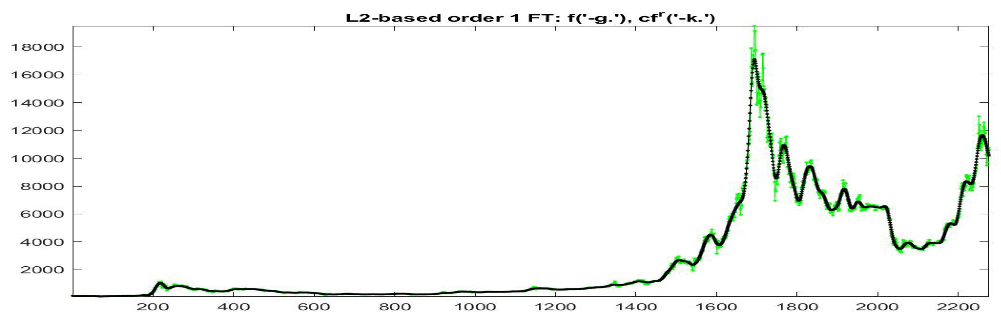
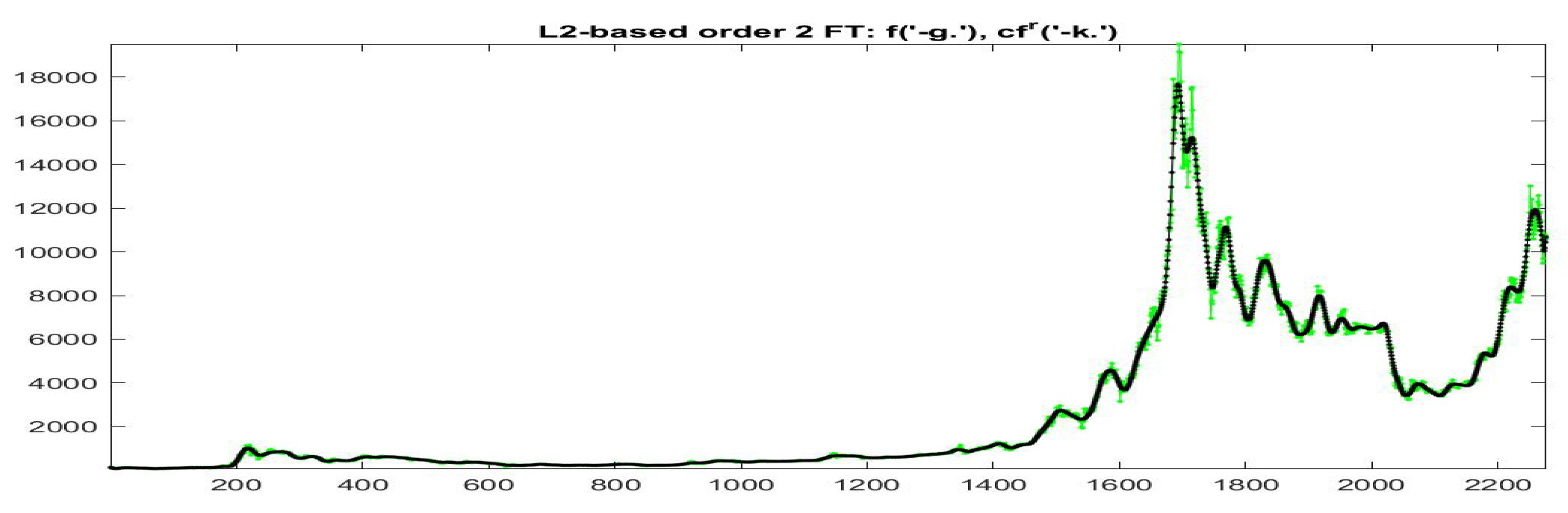
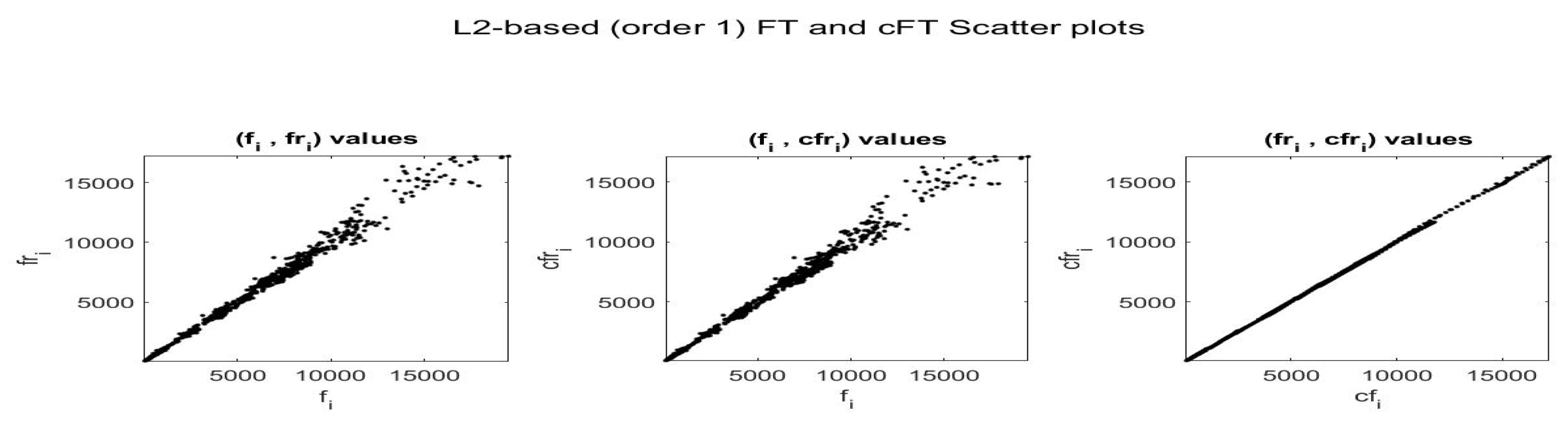
Essentially, we identify the elements of each cluster by its centroid and we estimate its goodness in terms of the vicinity between the modified version $f_{c,({\mathbb{P}}_a,\mathbb{A},r)}^q\left(t\right)$ at times $t_j=1, \dots , M$ and the observed data $f_j=BitCoi{n}_j$. In Figure 19 and Figure 20 the data $f_j$ (green colors) and $f_{c,({\mathbb{P}}_a,\mathbb{A},r)}^q\left(t_j\right)$ (black colors) are plotted for all the data with $r=4$ and $r=7$, respectively; remark in particular that the iF-transform values and the modified values have a very high correlation and the two values are very near each other on the whole range of small and big values of observed prices.

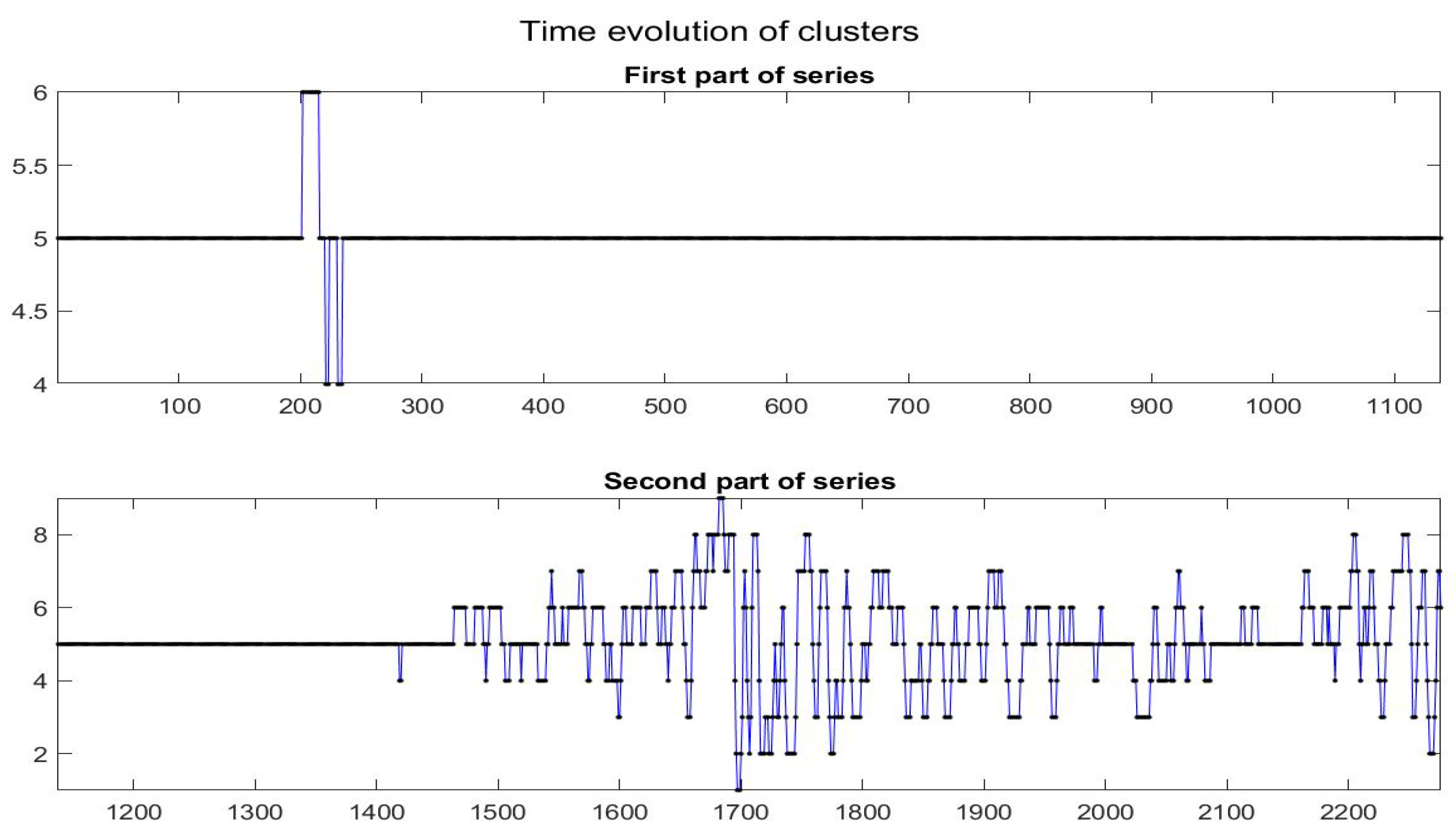
Finally, it is interesting to observe the time evolution of the different clusters (see Figure 21).

Remark that in the first part of the time series, the data (i.e., the local trends) persist into the quasi-zero slope (quasi-constant time series); after observation 1400, frequent changes in the local trends appear evident, but changes seem to be gradual from one class to a near one and only rarely the local trends jump from a form to a very different one. This appears clearly from the transition matrix $P=\left[prob(i,j)\right]$, $i,j=1,2, \dots , 9$ given below ($prob(i,j)$ is the probability that local trend of cluster i moves to class j): we see that matrix P is essentially tridiagonal.

P =		1	2	3	4	5	6	7	8	9
	1	0.57	0.29	0.14	0	0	0	0	0	0
	2	0.08	0.44	0.44	0	0.04	0	0	0	0
	3	0.02	0.12	0.39	0.25	0.12	0.03	0.05	0.02	0
	4	0	0.02	0.10	0.50	0.31	0.04	0.01	0.01	0
	5	0	0	0	0.03	0.93	0.03	0	0	0
	6	0	0	0.1	0.04	0.32	0.53	0.10	0.01	0
	7	0	0	0	0.03	0.04	0.27	0.56	0.10	0
	8	0	0.05	0.09	0.05	0	0.09	0.18	0.50	0.05
	9	0	0	0	0	0	0	0	0.50	0.50

4.2. F-Transform Fitting with Sparse r-Partition

The results obtained with the dense r-partition ${\mathbb{P}}_a$ are confirmed when using the sparse r-partition ${\mathbb{P}}_b$. The computations are performed only for the bandwidth $r=3$, corresponding to $n=326$ nodes of ${\mathbb{P}}_b$ and $42=2\ast 7\ast 3$ data belonging to each interval $\left[x_{k-r},xk+r\right]$.

Figure 22 and Figure 23 plot the local trends of orders $q=1$ and $q=2$, respectively (we have plotted only the second part of the Bitcoin time series).

The local trends are clustered into $nCl=9$ groups when $q=1$ and $nCl=15$ groups when $q=2$, pictured in Figure 24 and Figure 25. It appears that , for $q=1$, clusters 8 and 9 (and clusters 1, 13, 14, 15, when $q=2$) contain very few elements and possibly, in this sparse case, the number of clusters should be reduced to 7 and 11.

The substitution of estimated local trends with the ones obtained from centroids of each cluster, produces the smooth reconstructions represented in Figure 26 and Figure 27, respectively; the scatter-plots of the data and their smoothing with standard F-transform and the modified versions, are plotted in Figure 28 and Figure 29. We remark that corresponding to a stronger smoothing effect obtained with a smaller number of nodes in the decomposition (now it is sparse) the quality of the fitting is reduced.

5. Forecasting Bitcoin Prices with Gt100 Index

As described in the Introduction, there is empirical evidence that causal relationship between Bitcoin prices/returns and Google Trend scores is bi-directional and, we expect, this will be useful in designing short-term models that relate $BitCoin\left(t\right)$ to $GT100(t-l)$ for small values of lag $l\ge 1$. Clearly, as illustrated in sections three and four, the type of functional relationship will change with time and, in particular, the form of local polynomials is expected to persist only for short times around the actual time t and we can estimate their form (coefficients) from the data up to the last available observations.

In the setting of $L_p$-norm F-transform, we suggest using the (polynomial) direct F-transform components ${\vartheta }_k$ such as

$${\vartheta }_k\left(t\right)={\theta }_{k,0}+{\theta }_{k,1}(t-x_k)+ \dots +{\theta }_{k,q}{(t-x_k)}^q+{\theta }_{k,q+1}{g}_1\left(t\right)+{\theta }_{k,q+2}{g}_2\left(t\right)+ \dots +{\theta }_{k,q+s}{g}_s\left(t\right)$$

(39)

where ${\vartheta }_k$, $k= \dots , N-2,N-1,N$ is the k-th local trend function (k-th direct F-transform component) and $g_1\left(t\right), \dots , g_s\left(t\right)$ are delayed versions of the Google Trends $GT100\left(t\right)$ and/or $BitCoin\left(t\right)$ series.

We are interested to a forecasting model by which, with available observations of $BitCoin\left(t\right)$ and $GT100\left(t\right)$ at times $t= \dots , T-2,T-1,T$ up to time T, we like to construct a forecast of $BitCoin(T+l)$ for l steps ahead. To do this, we estimate the direct F-transform components (39) with appropriate q, s and values $g_1(t-l), \dots , g_s(t-l)$, obtained from observed values of $Bitcoin(t-l)$ and/or $GT100(t-l)$ for $t= \dots , T-2,T-1,T$; then, e.g., using the last estimated trend function ${\vartheta }_N\left(t\right)$ we approximate $BitCoin(T+l)$ with ${\vartheta }_N(T+l)$. This is always possible if the fuzzy r-partition is such that $T+l\in \left[T=x_N,x_{N+r}\right]$. Alternatively, if $r>1$, we can approximate $BitCoin(T+l)$ by computing the inverse F-transform at time $T+l$ as the combination of local trends ${\vartheta }_k(T+l)$ that have positive weights $A_k(T+l)$, the basic functions active at time $T+l$.

Clearly, this construction may be good and reasonable only for short-term forecasting. In our experiments we have used the first approximation only to forecast Bitcoin prices $BitCoin(T+l)$ with $l\in \left\{1,2,3,4,5\right\}$. The reported results are given for the last 1200 values of the available time series. We have used $q\in \left\{0,1,2\right\}$, $r\in \left\{1,2\right\}$ and two cases of functions $g_j\left(t\right)$:

Model A: $s=1$ and $g_1\left(t\right)=GT100\left(t\right)$;

Model B: $s=2$ and $g_1\left(t\right)=GT100\left(t\right)$, $g_2\left(t\right)=BitCoin(t-1)$, i.e., by adding an autoregressive term.

Our simple forecasting model is obtained by the following three steps:

Step 1. We start with one of the fitting model obtained in the analysis in previous sections and we chose the pair of values $(r,m_r)$ where $r\ge 1$ is the bandwidth of the r-partition and the associated value $m_r$ is the number of time observations used to estimate the parameters of local trend functions ${\vartheta }_k\left(t\right)$. We have found that $m_r$ observations on each subinterval of the partition, in the range $m_r=11, \dots , 25$, produces in general the best fitting results: two or three weeks of data are sufficient to obtain the forecast.

Step 2. The parameters in ${\vartheta }_k\left(t\right)$ are estimated using the L_p-norm-based criterion: we assume $p=1.5$ as a good intermediate value between quantile ($p=1$) and expectile ($p=2$) estimators.

Step 3. Each l-steps ahead forecast value $f_{T+l}$ for the last more recent 1200 available observations ending at time $T_{final}=2242$ is obtained from ${\vartheta }_N\left(t\right)$, where $N=2+r$ is the number on intervals in the partition covering $m_r$ data that terminate at time T: forecast $f_{T+l}$ is then estimated from data $BitCoi{n}_t,t=T-m_r+1, \dots , T$, $GT{100}_t,t=T-m_r-l+1, \dots , T-l$ for $g_1(t-l)$ and, in Model B, $BitCoi{n}_t,t=T-m_r-l+1, \dots , T-l$ for $g_1(t-l)$. In this way, we can compute $f_{T+l}={\vartheta }_N(T+l)$ as the needed values $g_1(T+l)=GT{100}_T$ and $g_2(T+l)=BitCoi{n}_T$ are available from observations.

For the fitting (i.e., with $l=0$) and forecasting models (with $l>0$) we report the mean square error ( $MSE=\frac{1}{m}{\displaystyle \sum _{i=1}^m}{(f_i-f_i^r)}^2$), the mean absolute percentage error ($\%MAE=\frac{100}{m}{\displaystyle \sum _{i=1}^m}{\displaystyle \frac{\left|f_i-f_i^r\right|}{f_i}}$) and the well-known Kendall $\tau$ rank correlation (a measure of ordinal association between $f_i$ and $f_i^r$).

We see from

Table 3. Approximation indices for $L_p$-norm F-transform of Bitcoin and GT100 For five values $p\in \left\{1,1.25,1.5,1.75,2\right\}$ and three orders $q\in \left\{0,1,3\right\}$ the table shows indices $MSE$, $\%MAE$, and Kendall $\tau$ correlation for the pairs $(f,f^{\left(r\right)})$ with $f\in \left\{Bitcoin,GT100\right\}$.

			Bitcoin			GT100
p	q	$MSE$	$\%MAE$	$\tau$	$MSE$	$\%MAE$	$\tau$
1	0	363.98	2.5173	0.9766	2.7670	7.8219	0.8897
1	1	201.66	2.0152	0.9815	1.8610	6.7139	0.9049
1	3	148.75	1.4739	0.9860	1.5614	4.8293	0.9331
1.25	0	219.72	2.5171	0.9768	2.3939	7.9307	0.8911
1.25	1	191.58	2.0315	0.9817	1.8211	6.8342	0.9074
1.25	3	139.34	1.4874	0.9863	1.4556	4.9210	0.9345
1.5	0	217.61	2.5641	0.9765	2.3339	8.1374	0.8910
1.5	1	190.20	2.0805	0.9814	1.8027	7.0240	0.9068
1.5	3	137.72	1.5284	0.9861	1.4169	5.1172	0.9331
1.75	0	217.79	2.6232	0.9762	2.3020	8.3932	0.8896
1.75	1	191.26	2.1298	0.9810	1.7920	7.2505	0.9057
1.75	3	137.75	1.5734	0.9858	1.4031	5.3430	0.9311
2	0	219.41	2.6859	0.9757	2.2855	8.6858	0.8877
2	1	192.74	2.1778	0.9708	1.7964	7.4879	0.9038
2	3	138.46	1.6155	0.9856	1.4040	5.5762	0.9289

that the fitting of Bitcoin and GT100 time series become significantly better by increasing the order q; it is also interesting to remark that GT100 fitting is much less precise that Bitcoin fitting (with the same p and q). On the other hand, polynomials of orders $q>1$ are not useful for extrapolation as they tend to be highly oscillating for a lag $l>1$.

For these reasons, only three pairs $(p,q)$ as in

Table 4. Model A: $L_p$-norm Fitting and Forecasting results For $p=1.5$, the table shows indices $\%MAE$ and Kendall $\tau$ correlation for the fitting (columns 4,5 with label $fit$) and the forecasting (columns 6,7 with label $for$) corresponding to five lags $l\in \left\{1,2,3,4,5\right\}$ and three pairs $(q,r)$ of order q and bandwidth r.

q	r	l	$\%\mathit{MAE}$-fit	$\mathit{\tau }$-fit	$\%\mathit{MAE}$-for	$\mathit{\tau }$-for
0	1	1	1.65	0.98	3.30	0.96
		2	1.67	0.98	4.41	0.95
		3	1.67	0.98	5.35	0.94
		4	1.58	0.98	6.17	0.93
		5	1.58	0.98	6.88	0.92
1	1	1	0.62	0.99	3.15	0.96
		2	0.59	0.99	5.08	0.94
		3	0.60	0.99	6.59	0.93
		4	0.60	0.99	8.09	0.91
		5	0.60	0.99	10.13	0.89
0	2	1	2.24	0.97	3.70	0.95
		2	2.28	0.97	4.77	0.94
		3	2.31	0.97	5.65	0.93
		4	2.22	0.97	6.43	0.92
		5	2.21	0.97	7.11	0.92

and

Table 5. Model B: $L_p$-norm Fitting and Forecasting results For $p=1.5$, the table shows indices $\%MAE$ and Kendall $\tau$ correlation for the fitting (columns 4,5 with label $fit$) and the forecasting (columns 6,7 with label $for$) corresponding to five lags $l\in \left\{1,2,3,4,5\right\}$ and three pairs of order q and bandwidth r.

q	r	l	$\%\mathit{MAE}$-fit	$\mathit{\tau }$-fit	$\%\mathit{MAE}$-for	$\mathit{\tau }$-for
0	1	1	1.56	0.98	3.21	0.96
		2	1.57	0.98	4.33	0.95
		3	1.56	0.98	5.31	0.93
		4	1.57	0.98	6.12	0.93
		5	1.57	0.98	6.83	0.92
1	1	1	1.17	0.98	3.16	0.96
		2	1.20	0.98	4.54	0.94
		3	1.17	0.98	5.84	0.93
		4	1.16	0.98	6.98	0.92
		5	1.18	0.98	7.89	0.91
0	2	1	1.56	0.98	3.21	0.96
		2	1.57	0.98	4.34	0.95
		3	1.56	0.98	5.31	0.93
		4	1.57	0.98	6.12	0.93
		5	1.57	0.98	6.83	0.92

are considered and we see that for forecasting, $q=1$ gives good results for small lag l while $q=0$ is better for higher lags.

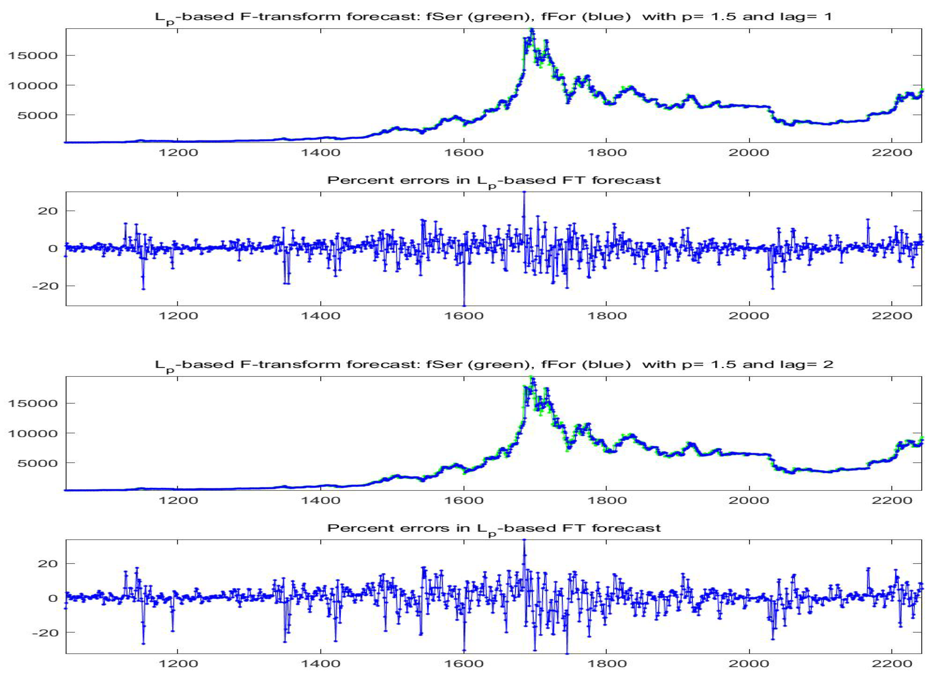
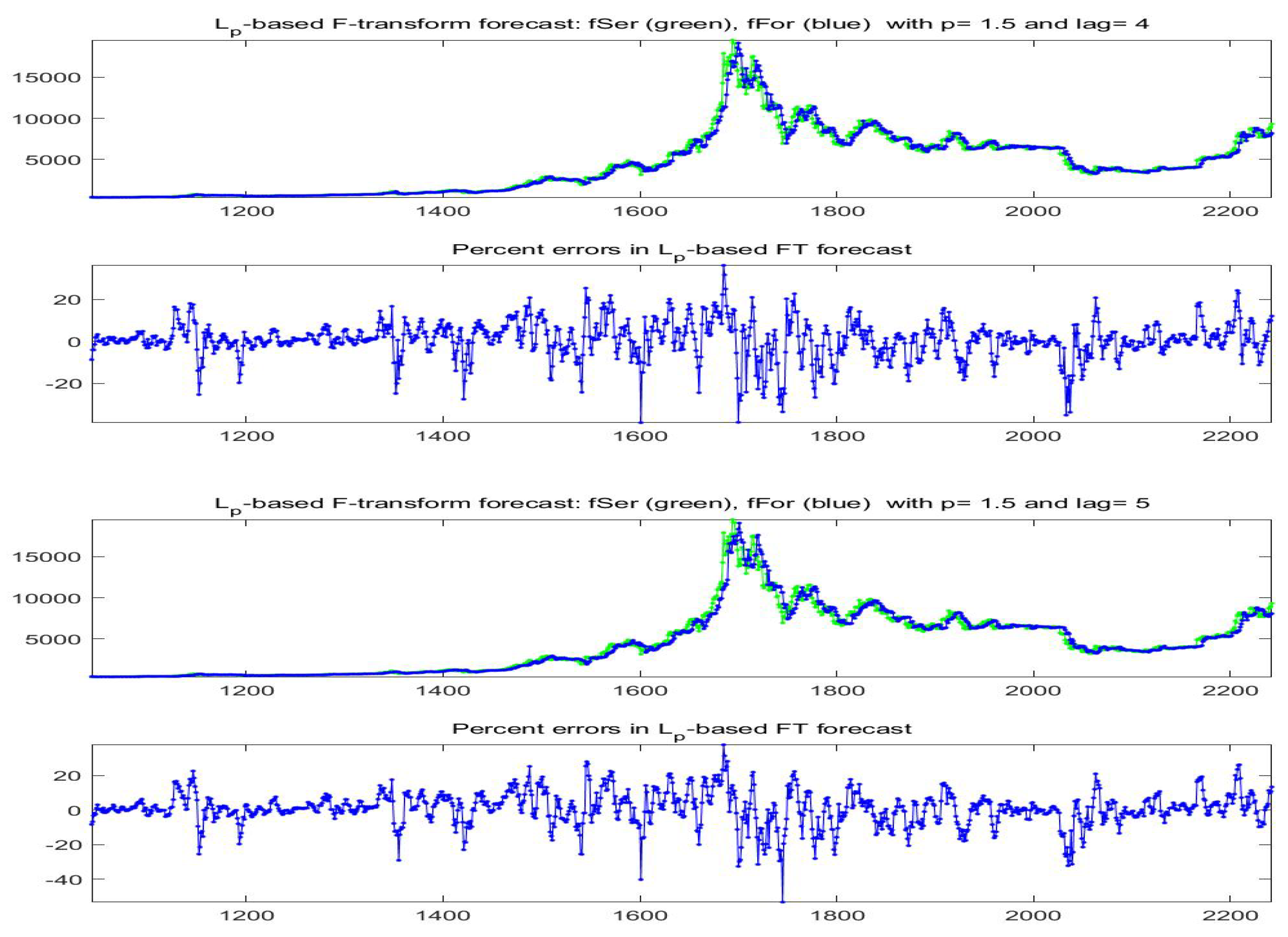
The forecast Bitcoin time series for lags $l=1,2$ obtained with model A are pictured in Figure 30; for lags $l=4,5$ and model B are plotted in Figure 31.

To conclude this section on forecasting Bitcoin time series, we shortly explore the statistical significance of the proposed models A and B. Following some ideas in [28], we compare our forecast estimates with the so-called random walk model, assumed as a benchmark for single step forecasting, i.e., with lag $l=1$. Defining the return series as $fRe{t}_t=log\left(\frac{fSe{r}_t}{fSe{r}_{t-1}}\right)$, the random walk forecast ${\widehat{r}}_T$ of the returns at time T is defined in terms of a fixed time horizon of s observations $fRe{t}_t$, $t=T-s+1, \dots , T$ ending at time T by

$$Re{t}_t={\widehat{r}}_T+{\epsilon }_t, {\epsilon }_t\sim ID(0,{\sigma }_T), t=T-s+1, \dots , T.$$

(40)

Then, considering that the return values $fRe{t}_t$ are known up to time T, the random walk forecast of $fRet$ at time $T+1$ is simply the average ${\widehat{r}}_T=\frac{1}{s}{\displaystyle \sum _{t=T-s+1}^T}Re{t}_t$, we can estimate the random walk forecast of $fSe{r}_{T+1}$ from the definition of return at time $T+1$ and obtain $f_{T+1}^{rw}=exp\left({\widehat{r}}_T\right)fSe{r}_T$. This calculations are performed for T being each of the last 730 available observations (two years).

As in [28], the Diebold–Mariano (DM) test statistics is applied to test the significance of the $MSE$ measures for our forecasts (with models A and B) in comparison with the random walk forecast. The results are reported in

Table 6. Diebold–Mariano test statistics for $L_p$-norm forecasting results The table shows indexes $sMSE=\sqrt{MSE}$ and Kendall rank correlation $\tau$, corresponding to lag $l=1$ forecasts for Models A and B, obtained with $p=1.5$, $q=1$ and bandwidth $r=1$.

	$\mathit{sMSE}$	DM-stat	p-Value	$\mathit{\tau }$
Model A	488.2	−2.9468	0.0016	0.9265
Model B	487.0	−3.8301	0.000064	0.9186
Random Walk	585.1	-	-	0.9078

.

Table 6 (in particular the small p-value) confirm that Bitcoin prices can be forecasted using F-transform of order $q=1$, as indeed both (simple) short-term models A and B outperform the random walk model.

6. Final Comments and Conclusions

In this paper, we apply the F-transform setting to analyze Bitcoin and the associated Google Trend time series. The direct and inverse F-transforms provide flexible and highly adaptive non-parametric smoothing in data analysis and they are adopted to develop a quantitative approach to sentiment analysis; considering empirical evidence, demonstrated in recent literature, that there is a bi-directional causal relationship between the two time series, we suggest a model to evaluate the dependence of Bitcoin prices on Google Trends scores and we show how and at which extend it is useful for short-term forecasting.

This research topic has rapidly increased in recent years and however deserves more investigation. Thanks to the high flexibility of smoothing techniques and modeling based on F-transform, we show that the web interest (querying) in Bitcoin phenomenon has an influence on the values of Bitcoin prices; the type and form of relationship has an essentially local nature as it may change from one period to the other. Remark that the reverse relationship remains important, but its interest is clearly less interesting.

In Section 3 and Section 4 the two time series are deeply analyzed in terms of non-parametric smoothing techniques, different clustering methodologies and efficient stylized fact research. Our results confirm the general hypothesis that short-term local trends characterize the Bitcoin time series, including the possibility to forecast its values at least for small steps ahead (from 1 to 5, daily, in our study).

Future research directions include improved clustering models identified by specific forms of local trends such as, e.g., exponential functions or other dependencies more suitable and stable for extrapolation than polynomials.

In the paper we do not argue about the superiority of forecasting based on F-transform with respect to many other methodologies; however, a comparison may be the opportunity to better investigate the theoretical properties in future research.

References

- Perfilieva, I. Fuzzy Transforms: Theory and Applications. Fuzzy Sets Syst. 2006, 157, 993–1023. [Google Scholar] [CrossRef]
- Perfilieva, I. Fuzzy Transforms: A Challenge to conventional transforms. In Advances in Images and Electron Physics; Hawkes, P.W., Ed.; Elsevier Academic Press: Cambridge, MA, USA, 2007; Volume 147, pp. 137–196. [Google Scholar]
- Perfilieva, I.; Novák, V.; Dvorak, A. Fuzzy transform in the analysis of data. Int. J. Approx. Reason. 2008, 48, 36–46. [Google Scholar] [CrossRef] [Green Version]
- Perfilieva, I. F-Transform. In Springer Handbook of Computational Intelligence; Kacprzyk, J., Pedrycz, W., Eds.; Springer: Berlin, Germany, 2015; Chapter 7; pp. 113–130. [Google Scholar]
- Kreinovich, V.; Kosheleva, O.; Sriboonchitta, S. Why Use a Fuzzy Partition in F-Transform? Axioms 2019, 8, 94. [Google Scholar] [CrossRef] [Green Version]
- Guerra, M.L.; Sorini, L.; Stefanini, L. Quantile and Expectile Smoothing based on L1-norm and L2-norm F-transforms. Int. J. Approx. Reason. 2019, 107, 17–43. [Google Scholar] [CrossRef]
- Guerra, M.L.; Sorini, L.; Stefanini, L. On the approximation of a membership function by empirical quantile functions. Int. J. Approx. Reason. 2020, 124, 133–146. [Google Scholar] [CrossRef]
- Bouri, E.; Gupta, R.; Tiwari, A.K.; Roubaud, D. Does Bitcoin hedge global uncertainty? Evidence from wavelet-based quantile-in-quantile regressions. Financ. Res. Lett. 2017, 23, 87–95. [Google Scholar] [CrossRef] [Green Version]
- Bellini, F.; Klar, B.; Muller, A.; Gianin, E.R. Generalized quantiles as risk measures. Insur. Math. Econ. 2014, 54, 41–48. [Google Scholar] [CrossRef]
- Bellini, F.; Bignozzi, V. On elicitable risk measures. Quant. Financ. 2015, 15, 725–733. [Google Scholar] [CrossRef]
- Daouia, A.; Girard, S.; Stupfler, G. Extreme M-quantiles as risk measures: From L1 to Lp optimization. Bernoulli 2019, 25, 264–309. [Google Scholar] [CrossRef] [Green Version]
- Bariviera, A.F.; Basgall, M.J.; Hasperuéb, W.; Naiouf, M. Some stylized facts of the Bitcoin market. Phys. A 2017, 484, 82–90. [Google Scholar] [CrossRef] [Green Version]
- Yermack, D. Is Bitcoin a Real Currency? An Economic Appraisal. In Handbook of Digital Currency: Bitcoin, Innovation, Financial Instruments, and Big Data; Chuen, D.L.K., Ed.; Academic Press: Cambridge, MA, USA, 2015; Chapter 2; pp. 113–130. [Google Scholar]
- Demir, E.; Gozgor, G.; Lau, C.K.M.; Vigne, S.A. Does economic policy uncertainty predict the Bitcoin returns? An empirical investigation. Financ. Res. Lett. 2018, 26, 145–149. [Google Scholar] [CrossRef] [Green Version]
- Corbet, S.; Lucey, B.; Urquhart, A.; Yarovaya, L. Cryptocurrencies as a financial asset: A systematic analysis. Int. Financ. Anal. 2019, 62, 182–199. [Google Scholar] [CrossRef] [Green Version]
- Gronwald, M. Is Bitcoin a Commodity? On price jumps, demand shocks,and certainty of supply. J. Int. Money Finance 2019, 97, 86–92. [Google Scholar] [CrossRef]
- Aharon, D.Y.; Qadan, M. Bitcoin and the day-of-the-week effect. Financ. Res. Lett. 2019, 31, 415–424. [Google Scholar] [CrossRef]
- Qin, M.; Su, C.; Tao, R. A new basket for eggs? Econ. Model. 2020. [Google Scholar] [CrossRef]
- Bouri, E.; Gupta, R. Predicting Bitcoin returns: Comparing the roles of newspaper- and internet search-based measures of uncertainty. Financ. Res. Lett. 2019. [Google Scholar] [CrossRef] [Green Version]
- Baiga, A.; Blaub, B.M.; Sabaha, N. Price clustering and sentiment in bitcoin. Financ. Res. Lett. 2019, 29, 111–116. [Google Scholar] [CrossRef]
- Zhang, W.; Wanga, P.; Li, X.; Shen, D. Quantifying the cross-correlations between online searches and Bitcoin market. Phys. A 2018, 509, 657–672. [Google Scholar] [CrossRef]
- Kristoufek, L. Power-law correlations in finance-related Google searches and their cross-correlations with volatility and traded volume: Evidence from the Dow Jones Industrial components. Phys. A 2015, 428, 194–205. [Google Scholar] [CrossRef] [Green Version]
- Eom, C.; Kaizoji, T.; Kang, S.H.; Pichl, L. Bitcoin and investor sentiment: Statistical characteristics and predictability. Phys. A 2019, 514, 511–521. [Google Scholar] [CrossRef]
- Karalevicius, V.; Degrande, N.; Weerdt, J.D. Using sentiment analysis to predict interday Bitcoin price movements. J. Risk Financ. 2018, 19, 56–75. [Google Scholar] [CrossRef]
- Kristoufek, L. BitCoin meets Google Trends and Wikipedia: Quantifying the relationship between phenomena in the Internet era. Sci. Rep. 2013, 3, 1–7. [Google Scholar] [CrossRef] [PubMed] [Green Version]
- Stolarski, P.; Lewoniewski, W.; Abramowicz, W. Chryptocurrencies Perceptions Using Wikipedia and Google Trends. Information 2020, 11, 234. [Google Scholar] [CrossRef]
- Dastgir, S.; Demir, E.; Downing, G.; Gozgor, G.; Lau, C.K.M. The causal relationship between Bitcoin attention and Bitcoin returns: Evidence from the Copula-based Granger causality test. Financ. Res. Lett. 2019, 28, 160–164. [Google Scholar] [CrossRef]
- Adcock, R.; Gradojevic, N. Non-fundamental, non-parametric Bitcoin forecasting. Phys. Stat. Mech. Its Appl. 2019, 531, 121727. [Google Scholar] [CrossRef]
- Atsalakis, G.S.; Atsalaki, I.G.; Pasiouras, F.; Zopounidis, C. Bitcoin price forecasting with neuro-fuzzy techniques. Eur. J. Oper. Res. 2019, 276, 770–780. [Google Scholar] [CrossRef]
- Trucios, C. Forecasting Bitcoin risk measures: A robust approach. Int. J. Forecast. 2019, 35, 836–847. [Google Scholar] [CrossRef]
- Kyriazis, N.A. A Survey on Empirical Findings about Spillovers in cryptocurrency Markets. J. Risk Financ. Manag. 2019, 12, 170. [Google Scholar] [CrossRef] [Green Version]
- Bohte, R.; Rossini, L. Comparing the Forecasting of cryptocurrencies by Bayesian Time-Varying Volatility Models. J. Risk Financ. Manag. 2019, 12, 150. [Google Scholar] [CrossRef] [Green Version]
- Xie, T. Forecast Bitcoin Volatility with Least Squares Model Averaging. Econometrics 2019, 7, 40. [Google Scholar] [CrossRef] [Green Version]
- Cretarola, A.; Figà-Talamanca, G.; Patacca, M. Market Attention and Bitcoin Price Modeling: Theory, Estimation and Option Pricing. 2017. Available online: https://papers.ssrn.com/sol3/papers.cfm?abstract_id=3042029 (accessed on 8 May 2019).
- Cretarola, A.; Figà-Talamanca, G.; Patacca, M. A continuous time model for bitcoin price dynamics. In Mathematical and Statistical Methods for Actuarial Sciences and Finance; Springer: Berlin, Germany, 2018; pp. 273–277. [Google Scholar]
- Chaim, P.; Laurini, M.P. Is Bitcoin a bubble? Phys. A 2019, 517, 222–232. [Google Scholar] [CrossRef]
- Panagiotidis, T.; Stengos, T.; Vravosinos, O. A Principal Component-Guided Sparse Regression Approach for the Determination of Bitcoin Returns. J. Risk Financ. Manag. 2020, 13, 33. [Google Scholar] [CrossRef] [Green Version]
- Moosa, I.A. The bitcoin: A sparkling bubble or price discovery? J. Ind. Bus. Econ. 2020, 47, 93–113. [Google Scholar] [CrossRef]
- Catania, L.; Grassi, S.; Ravazzolo, F. Forecasting cryptocurrencies under model and parameter instability. Int. J. Forecast. 2019, 35, 485–501. [Google Scholar] [CrossRef]
- Ji, S.; Kim, J.; Im, Ḣ. A Comparative Study of Bitcoin Price Prediction Using Deep Learning. Mathematics 2019, 7, 898. [Google Scholar] [CrossRef] [Green Version]
- Stavroyiannis, S.; Babalos, V.; Bekiros, S.; Lahmiri, S.; Uddin, G.S. The high frequency multifractal properties of Bitcoin. Phys. A 2019, 520, 62–71. [Google Scholar] [CrossRef]
- Yu, M.; Gao, R.; Su, X.; Jin, X.; Zhang, H.; Song, J. Forecasting Bitcoin volatility: The role of leverage effect and uncertainty. Phys. A 2019. [Google Scholar] [CrossRef]
- Zargar, F.N.; Kumar, D. Long range dependence in the Bitcoin market: A study based on high-frequency data. Phys. A 2019, 515, 625–640. [Google Scholar] [CrossRef]
- Zhang, Y.; Chan, S.; Chu, J.; Nadarajah, S. Stylised facts for high frequency cryptocurrency data. Phys. A 2018, 513, 598–612. [Google Scholar] [CrossRef]
- Takaishi, T. Statistical properties and multifractality of Bitcoin. Phys. Stat. Mech. Its Appl. 2018, 506, 507–519. [Google Scholar] [CrossRef] [Green Version]
- Da Silva Filho, A.C.; Maganini, N.D.; de Almeida, E.F. Multifractal analysis of Bitcoin market. Phys. A 2018, 512, 954–967. [Google Scholar] [CrossRef]
- Guerra, M.L.; Stefanini, L. Expectile smoothing of time series using F-transform. In Proceedings of the 8th Conference of the European Society for Fuzzy Logic and Technology (EUSFLAT 2013), Milan, Italy, 9–13 September 2013; pp. 559–564, ISBN 978-162993219-4. [Google Scholar]
- Coroianu, L.; Stefanini, L. Properties of fuzzy transform obtained from Lp-minimization and a connection with Zadeh extension principle. Inf. Sci. 2019, 478, 331–354. [Google Scholar] [CrossRef]
- Cont, R. Empirical properties of asset returns: Stylized facts and statistical issues. Quant. Financ. 2001, 1, 223–236. [Google Scholar] [CrossRef]
Figure 1.
Daily Bitcoin prices (blue color, left scale) and daily Google Trends series (red color, right scale) from 28 April 2013 to 17 June 2019.
Figure 2.
Scatter-plots of for daily Bitcoin prices (left picture) and daily GT100 trends (right), from April 2013 to June 2019.
Figure 3.
-based smoothing for Bitcoin (top picture, blue points) and GT100 (bottom, blue points) series, obtained with and . The green curves plot the observed series.
Figure 4.
Scatterplot of daily Bitcoin prices vs daily GT100 series. For this visualization, the two time series are normalized to the common range .
Figure 5.
The figure shows (inverse) -norm (on top) and -norm (on bottom) iF-transform functions obtained for the observations ; here, the daily Bitcoin prices are considered to be functions in the domain of GT100.
Figure 6.
Fuzzy-valued Espectile F-transform function of the data-set ; the five computed -cuts correspond to .
Figure 7.
The fitted time series (blue color) is obtained from -norm iF-transform function applied to the data-set ; the observed values are green and the observed values are red.
Figure 8.
Clustering A: the fitted time series (blue colour) is obtained from -norm iF-transform function applied to the data-set ; the observed values are green and the observed values are red.
Figure 9.
Clustering A: for each cluster, the fitted subseries (blue colour) are obtained from -norm iF-transform function applied to the subset of data assigned to each cluster; the observed values are green.
Figure 10.
Clustering B: the fitted time series (blue colour) is obtained from -norm iF-transform function applied to the data-set ; the observed values are green and the observed values are red.
Figure 11.
Clustering B: the fitted time series is in blue colour; the observed values are green.
Figure 12.
Clustering C: the fitted time series (blue color) is obtained from -norm iF-transform function applied to the data-set ; the observed values are green and the observed values are red.
Figure 13.
The blue points correspond to the observations assigned to each cluster by clustering C. The red points give the centroid values relative to two variables and .
Figure 14.
Figure 15.
-norm F-transform components of order 1 for Bitcoin series. The fuzzy r-partition is with (top picture) and (bottom).
Figure 16.
-norm F-transform components of order 2 for Bitcoin series. The fuzzy r-partition is with (top picture) and (bottom).
Figure 17.
Clustering of -norm F-transform components (polynomials) of order 1 for Bitcoin series. The clusters correspond to the fuzzy r-partition with (bottom picture) and (top).
Figure 18.
Clustering of -norm F-transform components (polynomials) of order 2 for Bitcoin series. The clusters correspond to the fuzzy r-partition with (bottom picture) and (top).
Figure 19.
-norm modified iF-transform values (top: , bottom: ) for Bitcoin series. The fuzzy r-partition is with .
Figure 20.
Figure 21.
Time evolution of clusters obtained with the -norm F-transform smoothing of order 1 for Bitcoin series. The fuzzy r-partition is with .
Figure 22.
-norm F-transform components of order 1 for Bitcoin series. The fuzzy r-partition is with .
Figure 23.
-norm F-transform components of order 2 for Bitcoin series. The fuzzy r-partition is with .
Figure 24.
Clustering of -norm F-transform components (polynomials) of order 1 for Bitcoin series. The fuzzy r-partition is with .
Figure 25.
Clustering of -norm F-transform components (polynomials) of order 2 for Bitcoin series. The fuzzy r-partition is with .
Figure 26.
-norm modified iF-transform values for Bitcoin series. Here, and the fuzzy r-partition is with .
Figure 27.
Figure 28.
Pairwise scatter-plots of values , and using -norm F-transform smoothing of order for Bitcoin series. The fuzzy r-partition is with .
Figure 29.
Figure 30.
Model A: -norm F-transform forecast (denoted as fFor) for the last 1200 days of available data for Bitcoin series (observed time series is denoted as fSer). Here, , and two lags (top two pictures), (bottom). The percent errors are also plotted.
Figure 31.
Model B: -norm F-transform forecast (denoted as fFor) for the last 1200 days of available data for Bitcoin series (observed time series is denoted as fSer). Here, , and two lags (top two pictures), (bottom). The percent errors are also plotted.