Article

Model-Based Control Design of an EHA Position Control Based on Multicriteria Optimization

Karlsruhe Institute of Technology (KIT), 76131 Karlsruhe, Germany
*
Author to whom correspondence should be addressed.
Submission received: 27 October 2022 / Revised: 5 December 2022 / Accepted: 6 December 2022 / Published: 8 December 2022

Abstract

:
For the control of dynamic systems such as an Electro-Hydraulic Actuator (EHA), there is a need to optimize the control based on simulations, since a prototype or a physical system is usually not available during system design. In consequence, no system identification can be performed. Therefore, it is unclear how well a simulation model of an EHA can be used for multicriteria optimization of the position control due to the uncertain model quality. To evaluate the suitability for control optimization, the EHA is modeled and parameterized as a grey-box model using existing parameters independent of test bench experiments. A method for multi-objective optimization of a controller is used to optimize the position control of the EHA. Finally, the step responses are compared with the test bench. The evaluation of the step responses for different loads and control parameters shows similar behavior between the simulation model and the physical system on the test bench, although the essential phenomena could not be reproduced. This means that the model quality achieved by modeling is suitable as an indication for the optimization of the control by simulation without a physical system.

1. Introduction

For fast linear movements under high loads, highly integrated Electro-Hydraulic Actuators (EHA) are often used in aerospace and industrial applications as an alternative to conventional hydraulic actuators. An EHA is a self-contained actuator that operates by electrical power. EHAs consist of at least a hydraulic cylinder, a hydraulic line system, a hydraulic pump, a motor, and power electronics.
Implementing a closed-loop position control for an EHA is difficult due to nonlinearities [1] and uncertainties such as friction or the dynamics of the piston pump [2]. Therefore, a primary research focus is the development and validation of different control approaches. For this purpose, classical Proportional–Integral–Derivative (PID) control, control including fuzzy logic [3,4,5], observer-based controls [6,7,8,9,10,11], adaptive trajectory controls [12,13], sliding mode control [14,15,16], or hybrids of the named approaches [17] are used to solve this problem. For application, the parameterization method is also of great importance in addition to the investigation of control schemes.
There are different methods for adjusting controls: metaheuristics, analytical methods, and multi-objective optimization, some of which rely on machine learning. For metaheuristics and other manual experience-based “trial-and-error” approaches, as often performed in industry, a high effort is required, especially if multiple operating points, such as different loads, need to be tested. Therefore, these methods are primarily used when a physical EHA, but not a suitable model of an EHA, is available for testing.
The mathematical modeling in terms of poles and zeros for the use of analytical methods is difficult for the EHA, since nonlinearities, such as friction and uncertainties in the parameterization, can lead to significant deviations in the overall result. A solution to overcome this problem is the system identification of a physical EHA on a test bench. Izzuddin et al. [18] obtained a linear transfer function in discrete form from multi-sine, as well as continuous step input via Auto-Regressive Exogenous (ARX) system identification, and compared control algorithms on the obtained simulation and tests on the test bench. Similar approaches were used to obtain an ARX model from experimental data and to validate the same controller in simulation and on the test bench, which was used to gather the input for system identification [19,20,21]. Since a physical system must be available to perform the system identification, this approach is unsuitable for early design optimization in product development, where mature prototypes are unavailable.
In addition to the previously mentioned approaches, a frequently used approach is a model-based optimization of the control system. For example, Wonohadidjojo et al. [22] developed an analytical model of the electrohydraulic servo system for PID optimization with Particle Swarm Optimization (PSO), modeling friction and internal leakage. Shern et al. [23] used a PID optimization with improved PSO, which chose between optimization of settling time or overshoot for the analytical model. The PSO was improved by combining two fitness functions for overshoot and settling time with linear weight summation [24]. Other optimization algorithms used for PID optimization for an EHA were, for example Genetic Algorithms [25,26,27], the Nelder–Mead approach [28], a hybrid algorithm of PSO, and gravitational search algorithms [29] or beetle antennae search algorithms [30].
Performance validation is either based on simulations or simulations and bench testing separately, similar to the development of other control methods. Comparison of simulation results with test bench results is not conducted, except in cases where the simulation model is parameterized with test bench results, by system identification, usually with the ARX model. In early product development, there is usually no physical EHA that can be tested on a test bench. Thus, no data are available for system identification. The data available in the early stages of product development are generally limited to individual components, but not to the system behavior of the EHA.
For an early optimization of the controller in the early stages of product development, it is necessary to optimize the control with a simulation model that is independent of the measurement data from a physical EHA which was tested on a test bench beforehand. The problem is that the validity of simulation models of an EHA parameterized only by data of individual components is unclear, and thus control optimization cannot be performed.
Therefore, this paper investigates how to model an EHA with a grey-box model. This grey-box model is used to optimize the controller parameters with a PSO. Finally, the optimized controller parameters are set on an EHA on a test bench, allowing the comparison of the dynamic behavior of the EHA on the test bench with the dynamic behavior of the simulation model. The main contributions of this article are summarized as follows:
  • Modeling of an EHA with a comprehensive grey-box model independent of data from bench tests, with the publication of all relevant parameters.
  • Application of a method for multi-objective optimization of PID control for optimal control parameters of the EHA using a simulation model and two load cases.
  • Comparison of the system behavior between the simulation model and the test bench with the help of step responses using the optimized control parameters for both load cases.

2. Materials and Methods

2.1. Electro-Hydraulic Actuator and Simulation Model

In this study, an EHA (BAS.50/32.U04.201.200 MI.BA100.G2.P42, AHP Merkle GmbH, Gottenheim, Germany) was investigated. The EHA consists of a double-acting hydraulic cylinder, a supply line system, an internal gear pump, and a permanent magnet-excited synchronous machine. The change in volume flow is continuous and unaffected by valve influences. Therefore, this EHA is a pump-controlled hydraulic system. Compared to valve-controlled systems, they are more efficient because there is no pressure drop (Manring and Fales 2019). An external inverter is used as power electronics to control the EHA (MOVIAXIS MXA81A-016-503-00/XFE24A, SEW-Eurodrive GmbH, Bruchsal, Germany).
In general, the method for multi-objective optimization of the PID position control is independent of the modeling software and could have been performed with modeling software for multi-domain systems such as MATLAB Simscape or Simcenter Amesim. The simulation model in this paper was created with MATLAB 2020a using the extension Simulink (version 10.1). The fifth-order Dormand–Prince equation was used as a fixed step solver. At first, subsystems were created based on their function. Those can be described with the process elements of transformer, converter, source, and sink. Figure 1 shows all subsystems of the simulation model on the top level of the description. Power quantities are exchanged between these subsystems. Examples of power quantities are the current and the voltage U for the electrical power or the torque M and the speed n for the mechanical rotary power. The central element is the control unit (CU), which adjusts the motor’s rotational velocity based on the desired position.
In the following, the subsystems control unit (CU), power electronics (PE), electric motor (EM), hydraulic pump (HP), hydraulic system (HS), and hydraulic cylinder (HC) are briefly described. It is specified which physical effects are taken into account or are neglected. All relevant parameters are listed in Appendix A. The subsystem load (L) is described in Section 2.3. Test bench for validation of the simulation model.

2.1.1. Control Unit (CU)

The control unit contains the parts concerning the position control of the hydraulic cylinder. In this study, the type of control is a PID feedback control. The controller is implemented as a discrete parallel PID controller using the PID blockset of MATLAB Simulink library. The controller uses a sampling frequency of 2 kHz. The position signal is influenced by external effects, which are indicated by noise. This noise can be characterized by a system identification of the used position sensor in the EHA. Three relevant frequencies of white noise with different amplitudes can be identified, which are described in Table 1. These white noises are added to the position signal and filtered with a kHz low-pass filter.

2.1.2. Power Electronics (PE)

The power electronics consist of a torque-based, field-oriented controller for the internal permanent magnet synchronous motor (PMSM) and an outer-loop speed controller. Therefore, the “Interior PM Controller” model from the powertrain blockset of the MATLAB Simulink library was used [32,33,34,35,36]. The overall inverter efficiency is constant. The current controller uses a sampling frequency of 16 kHz. The “Interior PM Controller” model is able to calculate the optimum current regulator gains based on the parameters of the electric motor. The chosen parameters are listed in Table A1 in the Appendix A.
An outer-loop speed controller was implemented, which is a PI feedback control based on the control unit of the inverter of SEW [37]. The acceleration pre-control gain is set to zero. The parameters are taken from the configuration on the test bench.

2.1.3. Electric Motor (EM)

The electric motor is modeled as a three-phase Interior Permanent Magnet Synchronous Motor (PMSM) with sinusoidal back electromotive force. For this purpose, the “Interior PMSM” model from the Powertrain blockset of the MATLAB Simulink library is used [38,39]. Torque is used as the mechanical input. Physical inertia, viscous damping, and static friction are considered in the model.

2.1.4. Hydraulic Pump (HP)

The hydraulic pump is an internal gear pump modeled as a gray box. The assignment between mechanical and hydraulic energy is performed with a black box model via a data sheet provided by the manufacturer. The speed and the pressure difference are used to determine the torque to be applied by the electric motor. The correlations between the parameters are integrated with a lookup table using the Akima spline as an interpolation and extrapolation method.
Due to the experimental determination of the data, this includes leakage and friction, but only for stationary conditions. Thus, the losses considered are independent of acceleration and pressure changes. The influence of rotational inertia is considered in the electric motor subsystem.
The volumetric flow rate is calculated using the volumetric displacement per rotation unit and the rotational speed. Compressibility is neglected so that incoming and outgoing volumetric flows are equal in magnitude. Since we only consider step responses in our study, we have also neglected the thermal aspect of the fluid system, which is otherwise very relevant. An example of the consideration of temperature and power dissipation is shown in [40]. Therefore, all fluid parameters are time-invariant and independent of pressure or temperature.

2.1.5. Hydraulic System (HS)

The hydraulic system describes all hydraulic parts except the hydraulic pump and cylinder. Therefore, the supply pipes between the hydraulic pump, cylinder, and reservoir are modeled. The hydraulic diagram of the hydraulic system is depicted in Figure 2.
The behavior of the supply pipes is characterized by the pressure loss Δ p due to local hydraulic resistances in the pipelines and their elbows. The pressure loss Δ p is calculated with the Darcy–Weisbach equation (Equation (1)) and is dependent on the pressure loss coefficient ζ , which is determined differently for pipe friction and the pipe elbow (Equation (2)). All other parameters such as the density ρ o i l , viscosity μ o i l , etc. are considered to be time-invariant. The compressibility of the fluid is neglected. The pressure losses are therefore dependent on the volume flow V ˙ .
Δ p = ζ ρ o i l 2 ( V ˙ A ) 2
ζ = ζ p i p e + ζ e l b o w
In the case of pipe friction, the pressure loss coefficient ζ p i p e (Equation (3)) is determined via the Darcy friction factor λ (Equation (4)), which depends on the Reynolds number R e (Equation (5)). For transient flow, the Hagen–Poiseuille equation is used. For turbulent flow in smooth conduits, the Blasius correlation is utilized. A Reynolds number greater than 100,000 is not expected.
ζ p i p e = λ L R
λ = { 64 R e ,     R e < 2320   ( t r a n s i e n t ) 0.3164 R e 0.25 ,     100 , 000 > R e 2320   ( t u r b u l e n t )
R e = 2 r | V ˙ | A μ o i l
The pressure loss in the elbow ζ e l b o w is characterized by the tabulated pressure loss coefficient provided in the Crane Technical Paper [41]. The hydraulic resistances can thus be transferred into characteristic diagrams and calculated separately for both supply pipes. The pipes are considered stiff and the compressibility of the hydraulic fluid is neglected. Therefore, the capacity and inductivity of the pipes are not considered. There is no leakage. The inertia of the hydraulic fluid is considered.
The reservoir must maintain the system pressure. Therefore, it contains a valve that opens when the pressure falls below the expected system pressure. Hydraulic fluid is flowing into the system and is therefore increasing the applied pressure.

2.1.6. Hydraulic Cylinder (HC)

The hydraulic cylinder is a double-rod linear actuator. The modeling is based on the description of Glöckler [42] and uses a force equilibrium. In this subsystem, due to the high pressures and large volumes, the compressibility of the hydraulic fluid is taken into account. The stiffness of the oil column in the cylinder depends on the bulk modulus of the hydraulic oil. The elasticity of the cylinder barrel is neglected.
The volumetric flow of the hydraulic fluid into the actuator is controlled by the output flow of the hydraulic system. The internal leakage is not considered, because it is equal to zero for new systems. The friction force F F r is modeled as Coulomb friction F C for static states and viscous friction for dynamic states. The Coulomb friction is constant and the viscous friction is linear dependent on the velocity of the hydraulic cylinder, see Equation (6). All fluid parameters are time-invariant. They are therefore assumed as temperature-independent.
F F r =   s g n ( x ) ( F C + f v i s c o u s | x | )
All relevant parameters are listed in Appendix A.

2.2. Method for Multi-Objective Optimization of PID Control

A method for the optimization of a PID control proposed in [43] is used to optimize the PID parameters of the presented EHA using the simulation model. The method is based on a multi-step incremental optimization of the multi-dimensional problem. First, the method is briefly presented. Second, the parameters selected in this study are presented.
For this method, the following five criteria are used: Integrated Time Weighted Square Error (ITSE) criterion Q I T S E , the Q t r , the settling time Q t s , the overshoot Q h O and the noise Q N o i s e . The mathematical equation of the target functions is shown in Equations (7)–(11). For the EHA, the variables error e , actual position y , step height of the input variable U s , and time of overshoot t h O , settled final position y f i n a l and the speed of the motor as the output of the controller n are used.
Q I T S E = 0 t e 2 ( t )     d t
Q t r = t 1 ( y = 0.9 U s ) t 0 ( y = 0.1 U s )
Q t s = t ( | y ( t ) U s U s | < 0.1 ) t h O
Q h O = max ( y ( t ) y f i n a l ) y f i n a l
Q N o i s e = | n ( t ) |
The PID values are optimized using the five criteria presented with a cost function. The main criterion f 1 shift a percentage of the exponent with a certain weight g . The weight g is selected by the user. Furthermore, the exponential function of the main criterion forms a valley around the desired absolute value. The partial costs of the secondary criteria f 2 , on the other hand, have continuously decreasing costs towards lower values. This forces the optimization algorithm to search for a solution on the multidimensional Pareto front, which lies around the desired value of the shifted main criterion.
f 1 ( x , x r e f , α , g ) = e α | x g x r e f x r e f |
f 2 ( x , x r e f , α ) = e α x x r e f x r e f
Furthermore, criterion f 3 is introduced that represents stability criteria and nonlinear boundary conditions. This results in the overall cost function, which is represented by the following equation.
F ( x 1 , , x n ) = i = 1 n f 1 ( x i , x i , r e f , α i ) f 2 ( x k , x k , r e f , α , g ) f 3 ( s ) , i A ,   k B A = { 1 , , n } ,     B = { 1 , , n } ,     A B
The method uses an iterative and relative approach for optimization. Based on the created model, the first step is to determine the possible search space for the PID parameters. In this study, the method of Ziegler and Nichols is used to determine a first—mostly non-matching—parameter set of PID values. Subsequently, an initial optimization is performed with the PSO algorithm. The purpose of this step is to obtain a rough estimate which reflects the system-dependent behavior. The optimization uses only the ITSE criterion Q I T S E . With the obtained PID values the first set of criteria can be determined. These initial values are used to calculate the above mentioned normalization. Based on the nature of a Pareto-optimal problem, the secondary criteria will be degraded during this optimization. If the optimization result does not correspond to the desired goal, another cycle can be started. Here, the main criterion and an associated improvement with the weight g are defined. The result of the previous optimization is used as a reference.
For this study, the objective of controlling the EHA is defined as follows: Reaching the set point as quickly as possible without considerable overshoot and with a smooth controller output. Therefore, three optimization loops are performed including the first optimization with the ITSE criterion. To achieve the control objective, the second optimization aims to minimize the control output by 20% (g = 0.8), and the third aims to reduce the overshoot by 20% (g = 0.8). The limits for PSO in the optimization loops refer to the previous parameters of Ziegler and Nichols, and the previous loop, respectively. The limits are 10% and 1000% for the proportional gain as well as 0.1% and 100,000% for the integral part and derivative part. Table 2 shows all setting values for the optimization in this study.

2.3. Test Bench for Validation of the Simulation Model

The focus of this study is on the position control of the EHA. To validate the simulation model, a test bench was used to measure and evaluate step responses. A step height of 5 mm is selected for this purpose, as 5% of the maximum stroke is a suitable test case [44].
The test bench is controlled by the measurement and control system Adwin-Pro2 (Jäger Computergesteuerte Meßtechnik GmbH, Lorsch, Germany). The EHA is controlled by an external inverter (MOVIAXIS MXA81A-016-503-00/XFE24A, SEW-Eurodrive GmbH, Bruchsal, Germany), which is coupled to the measurement and control system via an EtherCAT real-time network with a sampling frequency of 2 kHz. As described in the modeling, the control system of the EHA is a cascaded control system. The outer control loop of the EHA is closed with the help of a magnetostrictive linear position sensor (BTL0LP3, Baluff GmbH, Neuhausen auf den Fildern, Germany) via Adwin-Pro2. The position control is performed with a sampling frequency of 2 kHz. The other internal control loops (speed and current control) are implemented directly on the inverter. The speed control is performed with a sampling frequency of 4 kHz and the current control runs with a sampling frequency of 16 kHz. The control system, the systems involved, and the measurement equipment used are shown in Figure 3.
Two modules are used as loads. In the first load case, an inertial load realized with weights is applied to the EHA. A mass of 11.83 kg was chosen as the weight. The mass is shown in Figure 4a. In aerospace applications, the load increases due to the wind when the actuator extends the wing flap. Therefore, the actuator is moved against a compression spring for the second load case. A spring stiffness of 241.381 N/mm was selected for validation. The compression spring is shown in Figure 4b.

3. Results

In this section, the optimization results of the PID control based on the simulation model are presented. The simulation model is validated by comparing the various step responses of the simulation model with the step responses obtained on the test bench.

3.1. Results of the Method for Multi-Objective Optimization of PID Control for the Simulation Model

The results in this section were obtained using the simulation model of the EHA. According to the optimization method, initial parameters were first extracted for Ziegler and Nichols. As shown in Table 2, the search space for the PSO is determined based on these initial parameters. For the inertial load, the results of Ziegler and Nichols, the system characterization based on the ITSE criteria, and the optimization loops based on overshoot and rise time are shown in Table 3. The corresponding step responses are shown in Figure 5.
For the spring load, the results of Ziegler and Nichols and the three optimization loops are shown in Table 4. The corresponding step responses are shown in Figure 6.

3.2. Validation of the Simulation Model for the Electro-Hydraulic Actuator

To validate the simulation model, a comparison is made between the simulated step responses and those measured on the test bench. The step responses for the inertial load using the PID parameter set of Table 3 are shown in Figure 7. The step responses for the spring load for the PID parameters of Table 4 are shown in Figure 8.
The validation results from Figure 7 are described in the following. For Ziegler and Nichols, the step response shows approximately similar behavior with a significant deviation in overshoot and a deviation in rise time. For the system characterization, there are also deviations: While the slope is similar at the start, a sudden change of the gradient can be observed on the test bench at the amplitude of 4 mm. Furthermore, the overshoot is significantly lower for the test bench. For the first optimization loop, a similar behavior except for a smaller overshoot is obtained. For the second optimization loop, a similar behavior with only a tiny change of the gradient at 4 mm is observed.
The validation results from Figure 8 are described in the following. The validation results for the spring load also show significant differences for all four parameter sets. Partially, the results are similar to those for the inertial load in Figure 7. Therefore, the differences in the inertial load are also described.
For Ziegler and Nichols, the step response shows approximately similar behavior to the inertial load. For system characterization, the step response shows approximately similar behavior to the inertial load, except that the settling time of the test bench results is much slower. For the first optimization loop, the results differ significantly: the overshoot is much more significant in the simulation. For the first optimization loop, as shown in Section 3.1, the simulation results show a permanent deviation due to the small integral part. The permanent deviation is not observed on the results of the test bench. For the second optimization loop, in contrast to the inertial load, different behavior is shown. Although the overshoot is the same, it occurs later, and the settling time is significantly slower for the test bench results.

4. Discussion

In this section, the results of the method for multi-objective optimization of PID control on the simulation model are discussed. Then, the validation of the simulation model using a test bench is discussed as the main result. Finally, limitations and further research directions are elaborated.

4.1. Discussion of the Results of the Method for Multi-Objective Optimization of PID Control

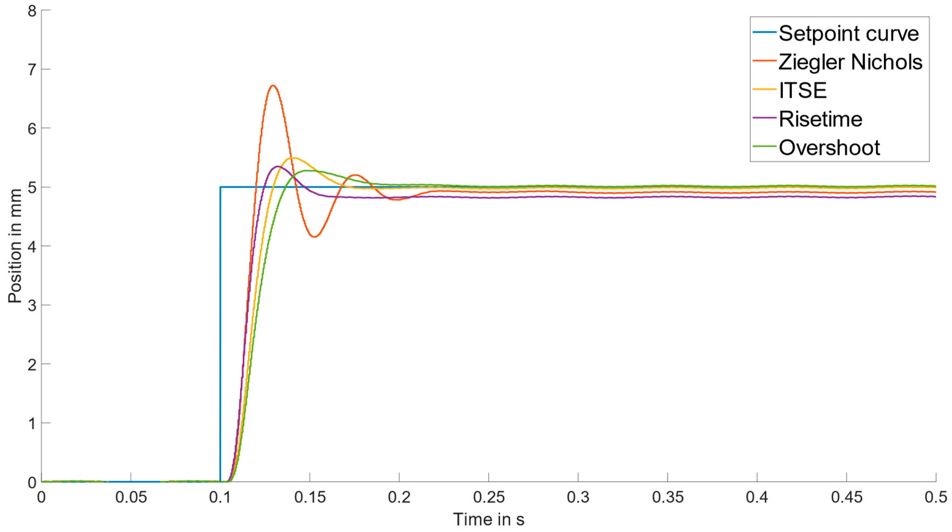
The results show the expected results for the inertial load in Figure 7 for the four parameter sets. While there is a strong overshoot in Ziegler and Nichols, as expected, the three optimizations show a local Pareto-optimum concerning the primary optimization criterion. From the PID values in Table 3, it can be seen that the proportional gain differs significantly. For the optimization of rise time, a high derivative part and a low integral part are found. For the optimization of ITSE and overshoot, a high integral part and a low derivative part are found.
The results for spring loading in Figure 8 also show the expected results in all cases. The results are similar to those for the inertia. For Ziegler and Nichols, almost similar behavior was obtained with the same PID values, but a permanent deviation occurs due to the constant force of the compressed spring. The PID values of Table 3 and Table 4 differ mainly in the significantly higher integral part. As expected, the derivative part is most significant for the rise time with the smallest integral part.
The results show that the optimization method, which was designed and validated on rotating systems, also works for translational systems such as the EHA. For the validation of the simulation, the method must reach different local optima so that the validation can be performed with different PID values. Thus, the method has served its purpose and the local optima are suitable for validating the simulation. The use of both loads has proven to be suitable since, in this way, different integral parts and also different operating points can be validated.
The selection of the best PID values depends on the requirements of the overall system, for example, how fast the system should respond and how significant the overshoot should be. The method is thus a suitable way to optimize the PID control based on simple predefined objectives. However, a valid simulation model is a prerequisite. Therefore, the simulation model was validated in Section 3.2 by comparing these step responses with the step responses obtained on the test bench.

4.2. Validation of the Simulation Model with the Test Bench

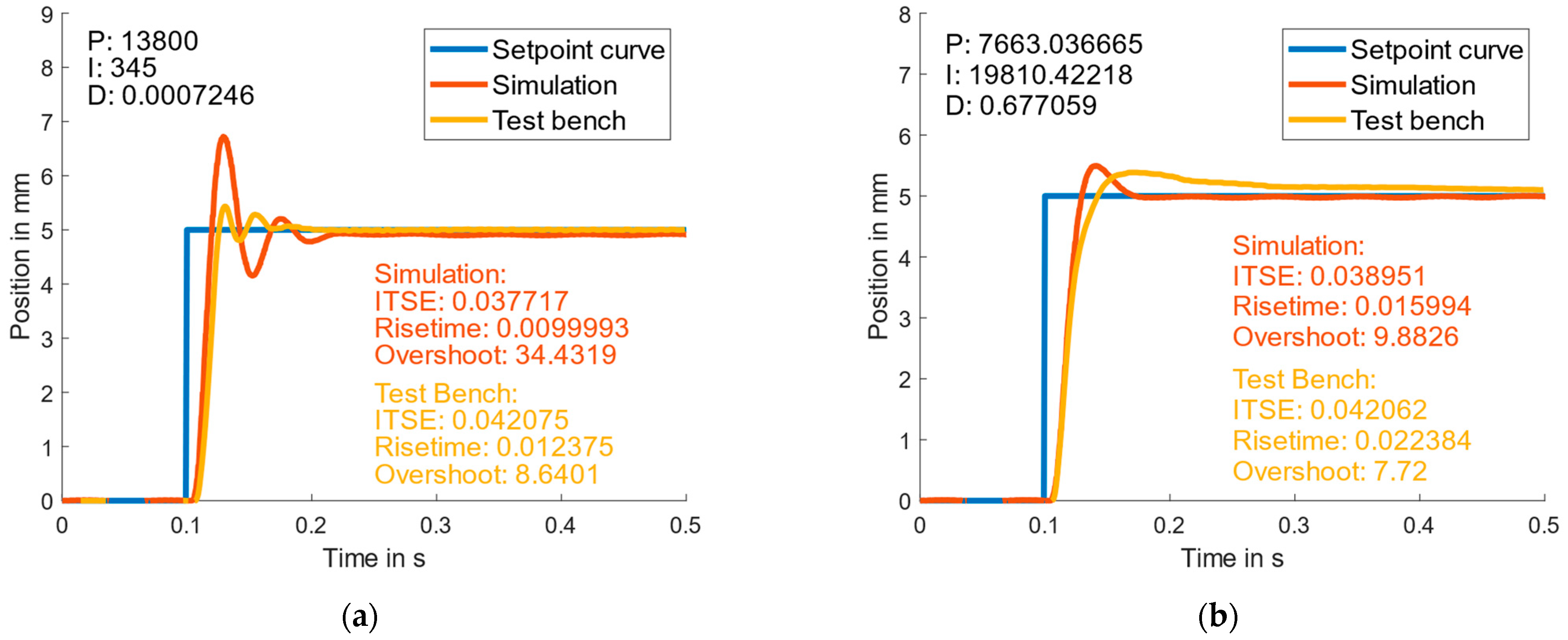
The validation results for the four parameter sets of the inertial load show partially significant differences between the step responses obtained with the simulation model and on the test bench.
The deviation of the rise time is due to different behavior between the results of the simulation and test bench. While the increase in the position of the paths is similar at the beginning, a sudden change in the slope is observed on the test rig at an amplitude of 4 mm in most cases. Examples are the system characterization, first and second optimization loop for inertial load, where the change of the gradient is present in different magnitudes. For the second optimization loop, a similar behavior with only a tiny change of the gradient at 4 mm is observed. This can be explained by an oscillation between the outer loop of the position controller and the inner loop of the speed controller, which is shown in Figure 3. This oscillation is not adequately represented in the simulation model for the shown operating points shown. A second explanation is the influence of a limitation in the inverter, which was not represented in the simulation.
The deviation in overshoot is due to the damping of the system, which is difficult to simulate in absolute values. It seems that the hardware system has a higher damping coefficient than in the simulation. A second cause is probably the previously discussed change in the gradient.
Another phenomenon is the different response to a high integral part of the controller in the spring load. While the simulation quickly reaches the setpoint at a high integral part, a low integral part results in a permanent offset of the amplitude. The results of the test bench reach the setpoint very slowly at a high integral part of the controller. With a low integral part, the settling time is very slow. This could be explained by the control implemented in the inverter. It must be noted that modeling the control implemented in the inverter is a highly complex task, since not all information, such as the stored motor model, are available. Furthermore, it is unclear how the internal filters of the inverter are designed in detail.
Overall, by comparing the step responses of the simulation model with the test bench results for the inertia or spring load, the key phenomenon is the change in slope at an amplitude of 4 mm, which can be explained by the interaction of the cascaded control on the test rig, across almost all results.
The deviation between the results obtained with the simulation model and with the test bench shows that the simulation model of an EHA parameterized only on data of individual components is not completely valid for control optimization. Nevertheless, it indicates the behavior of the control system that can already be used in product development if no physical EHA is available. Thus, the modeling approach and the modeling itself provide added value to the application. If a physical EHA is available, performing a system identification, e.g., via Regressive Exogenous (ARX), as conducted by [19,20,21], can be performed to obtain a better fit between the results of the simulation model and the test bench.

4.3. Limitations and Further Research Directions

The results show a strong dependence of the internal control loop on the speed of the inverter. Therefore, modeling and validation of the internal control loop should be a basic prerequisite for the successful execution of a grey-box or white-box simulation. However, if the internal control of the simulation model is not matched to the test bench at a high level of detail, the probability of success is low. In this case, interactions in the cascaded control, as in our study, can influence the overall result. One possibility would be to use the method for optimizing the PID control to parameterize the speed control loop in the simulation model.
The quality of the grey-box simulations depends mainly on the amount and quality of the available data and information. In our case, we had many parameters available, as can be seen from Appendix A. The problem was mainly the lack of information about the cascaded control. Thus, the success of a similar approach depends on the available information.
In the grey-box simulation, many phenomena, such as sensor noise, were implemented. However, there are other phenomena, such as the capacity and inductivity of the pipes, that could have been improved with the appropriate information. To fully evaluate the system reliability of the EHA with the optimized position control used here, the thermal domain would also need to be considered, as temperature also has an impact on the dynamics of the system.
In our study, we investigated an EHA with two loads at a defined step response. Only some of the operating points that the EHA can perform were investigated. More operating points, and also other EHA, should be considered for transferring the results. This does not affect the core statement of this work, which is that the grey-box simulation is only suitable as an indication for control optimization. This can be assumed because the difficulties are present in all EHAs, especially due to the cascaded control. Instead, the amount and quality of information, as mentioned above, take an overriding role.
Given the already achieved convergence of results when using a grey-box model, there is still great potential and further research directions. Future work should investigate if it is possible to obtain better results with more information. To draw insights from the comparison, the representation of the parameters and the mapped phenomena or physical effects, as in this study, are necessary.
Another research direction is to use the simulation model of the EHA as a digital twin by connecting it directly to the EHA on the test bench. By continuously comparing the digital and physical EHA, the deviations can be identified and used to improve the simulation by parameterizing physical parameters, such as friction, that are difficult by generic white-box models. A high model quality can be achieved without relying on a black-box model, which can only be transferred to similar EHAs to a limited extent.
To fully evaluate the system reliability of the EHA with the position control optimized here, the thermal domain should also be considered as well, as temperature also has an impact on the dynamics of the system. For this purpose, thermal coupling systems must be used so that all relevant domains are also taken into account in the sense of the digital twin, to obtain a high degree of reliability concerning the findings obtained.

Author Contributions

Conceptualization, M.D.; methodology, F.L., K.W. and M.D.; software, F.L., K.W. and M.D.; validation, M.D.; formal analysis, F.L. and K.W.; investigation, M.D. and F.L.; data curation, M.D.; writing—original draft preparation, M.D., F.L. and K.W.; writing—review and editing, M.D., F.L., K.W., T.G. and S.M.; visualization, M.D. and F.L.; supervision, T.G. and S.M.; project administration, M.D.; funding acquisition, S.M. and T.G. All authors have read and agreed to the published version of the manuscript.

Funding

This research was funded by the Federal Ministry for Economic Affairs and Climate Action under the funding number 20Y1910E. The authors of this publication are responsible for its contents. The authors gratefully acknowledge the support.

Data Availability Statement

The data that support the findings of this study are available from the corresponding author upon reasonable request.

Conflicts of Interest

The authors declare no conflict of interest.

Abbreviations

The following abbreviations are used in this manuscript:
EHAElectro-Hydraulic Actuators
PIDProportional–Integral–Derivative
ARXAuto-Regressive Exogenous
PSOParticle Swarm Optimization
CUControl Unit
PEPower Electronics
EMElectric Motor
PMSMPermanent Magnet Synchronous Motor
HCHydraulic Pump
HPHydraulic System
HCHydraulic Cylinder
ITSEIntegrated Time Weighted Square Error

Appendix A

Table A1. Relevant parameters of the simulation model.
ParameterValue
Power Electronics (PE)
Current controller proportional gain D-axis12.6V/A
Current controller proportional gain Q-axis20.1V/A
Current controller integral part2320V/A∗s
Current controller bandwidth200Hz
Speed controller frequency2000Hz
Speed controller proportional gain10001/s
Speed controller integral part1001/s2
Setpoint speed filter0.63 × 10−31/s
Actual speed filter1.23 × 10−31/s
Acceleration precontrol filter1.25 × 10−3s
Electric Motor (EM)
Nominal speed401/s
Nominal torque24.8Nm
Maximal torque90Nm
Nominal power motor6200W
Reduced rotational inertia1566kg/mm2
Number of rotor polepairs5
DC link voltage560V
Nominal current13.8A
Current limit55.2A
D-inductance (field)10mH
Q-inductance (torque)16mH
Resistance (at 20°C)1.5
Flux linkage established by magnets0.214Vs
Factor of induced voltage0.137V(RMS)/rpm
Limit speed for static friction0.001rad/s
Static friction torque0.5Nm
Viscous damping0.005Nm*s/rad
Hydraulic System (HS)
Hydraulic fluid density864kg/m3
Hydraulic fluid bulk modulus1.448 × 109N/m2
System pressure2bar
Tube A length160mm
Tube B length420mm
Tube A inner radius9.0mm
Tube B inner radius9.0mm
Elbow A quantity1
Elbow B quantity3
Elbow bending radius40mm
Hydraulic Cylinder (HC)
Piston radius25mm
Rod radius16mm
Dead volume A-Side2.90 × 10−5m3
Dead volume B-Side2.90 × 10−5m3
Moving mass of piston and rod4.19kg
Coulomb friction force150N
Viscous friction coefficient200Ns/m

References

  1. Sohl, G.A.; Bobrow, J.E. Experiments and simulations on the nonlinear control of a hydraulic servosystem. IEEE Trans. Control Syst. Technol. 1999, 7, 238–247. [Google Scholar] [CrossRef] [PubMed]
  2. Doan, N.; Yoon, J.I.; Ahn, K.K. Position control of Electro hydrostatic actuator (EHA) using a modified back stepping controller. J. Korean Soc. Fluid Power Constr. Equip. 2012, 9, 16–22. [Google Scholar] [CrossRef] [Green Version]
  3. Kundu, S.; Bhattacharjee, R.; Chaudhuri, S. Evaluation of Fuzzy-Logic based Position Control Strategies for an Electrohydraulic Actuation System. In Proceedings of the 2021 International Conference on Advances in Electrical, Computing, Communication and Sustainable Technologies (ICAECT), Bhilai, India, 19–20 February 2021; pp. 1–7. [Google Scholar]
  4. Bessa, W.M.; Dutra, M.S.; Kreuzer, E. Sliding Mode Control with Adaptive Fuzzy Dead-Zone Compensation of an Electro-hydraulic Servo-System. J. Intell. Robot. Syst. 2010, 58, 3–16. [Google Scholar] [CrossRef]
  5. Guo, Q.; Shi, G.; Wang, D. Adaptive Composite Fuzzy Dynamic Surface Control for Electro-Hydraulic-System, with Variable-Supply-Pressure. Asian J. Control 2020, 22, 521–535. [Google Scholar] [CrossRef]
  6. Guo, K.; Wei, J.; Fang, J.; Feng, R.; Wang, X. Position tracking control of electro-hydraulic single-rod actuator based on an extended disturbance observer. Mechatronics 2015, 27, 47–56. [Google Scholar] [CrossRef]
  7. Nguyen, M.H.; Dao, H.V.; Ahn, K.K. Active Disturbance Rejection Control for Position Tracking of Electro-Hydraulic Servo Systems under Modeling Uncertainty and External Load. Actuators 2021, 10, 20. [Google Scholar] [CrossRef]
  8. Won, D.; Kim, W.; Shin, D.; Chung, C.C. High-Gain Disturbance Observer-Based Backstepping Control With Output Tracking Error Constraint for Electro-Hydraulic Systems. IEEE Trans. Control Syst. Technol. 2015, 23, 787–795. [Google Scholar] [CrossRef]
  9. Chao, Q.; Zhang, J.; Xu, B.; Huang, H.; Pan, M. A Review of High-Speed Electro-Hydrostatic Actuator Pumps in Aerospace Applications: Challenges and Solutions. J. Mech. Des. 2019, 141, 050801. [Google Scholar] [CrossRef] [Green Version]
  10. Yao, J.; Wang, P.; Dong, Z.; Jiang, D.; Sha, T. A novel architecture of electro-hydrostatic actuator with digital distribution. Chin. J. Aeronaut. 2021, 34, 224–238. [Google Scholar] [CrossRef]
  11. Yang, X.; Ge, Y.; Deng, W.; Yao, J. Observer-based motion axis control for hydraulic actuation systems. Chin. J. Aeronaut. 2022, in press. [Google Scholar] [CrossRef]
  12. Nguyen, M.T.; Doan, N.C.N.; Hyung, G.P.; Kyoung, K. Trajectory control of an electro hydraulic actuator using an iterative backstepping control scheme. Mechatronics 2015, 29, 96–102. [Google Scholar] [CrossRef]
  13. Yang, X.; Deng, W.; Yao, J. Neural Adaptive Dynamic Surface Asymptotic Tracking Control of Hydraulic Manipu-lators With Guaranteed Transient Performance. IEEE Trans. Neural Netw. Learn. Syst. 2022, 2022, 3141463. [Google Scholar] [CrossRef]
  14. Chen, G.; Liu, H.; Jia, P.; Qiu, G.; Yu, H.; Yan, G.; Ai, C.; Zhang, J. Position Output Adaptive Backstepping Control of Electro-Hydraulic Servo Closed-Pump Control System. Processes 2021, 9, 2209. [Google Scholar] [CrossRef]
  15. Cerman, O.; Hušek, P. Adaptive fuzzy sliding mode control for electro-hydraulic servo mechanism. Expert Syst. Appl. 2012, 39, 10269–10277. [Google Scholar] [CrossRef]
  16. Lin, Y.; Shi, Y.; Burton, R. Modeling and Robust Discrete-Time Sliding-Mode Control Design for a Fluid Power Electrohydraulic Actuator (EHA) System. IEEE ASME Trans. Mechatron. 2013, 18, 1–10. [Google Scholar] [CrossRef]
  17. Feng, L.; Yan, H. Nonlinear Adaptive Robust Control of the Electro-Hydraulic Servo System. Appl. Sci. 2020, 10, 4494. [Google Scholar] [CrossRef]
  18. Izzuddin, N.H.; Faudzi, A.M.; Johari, M.R.; Osman, K. System identification and predictive functional control for electro-hydraulic actuator system. In Proceedings of the 2015 IEEE International Symposium on Robotics and Intelligent Sensors (IRIS), Langkawi, Malaysia, 18–20 October 2015; pp. 138–143. [Google Scholar]
  19. Liang, X.W.; Mohd Faudzi, A.A.; Ismail, Z.H. System Identification and Model Predictive Control using CVXGEN for Electro-Hydraulic Actuator. Int. J. Integr. Eng. 2019, 11, 04018. [Google Scholar] [CrossRef]
  20. Ishak, N.; Yusof, N.M.; Azahar, W.N.A.W.; Adnan, R.; Tajudin, M. Model identifiction and controller design of a hydraulic cylinder based on pole placement. In Proceedings of the 2015 IEEE 11th International Colloquium on Signal Processing & Its Applications (CSPA), Kuala Lumpur, Malaysia, 6–8 March 2015; pp. 198–202, ISBN 978-1-4799-8249-3. [Google Scholar]
  21. Rahmat, M.F.; Rozali, S.M.; Wahab, N.A.; Jusoff, K. Modeling and Controller Design of an Electro-Hydraulic Actuator System. Am. J. Appl. Sci. 2010, 7, 1100–1108. [Google Scholar] [CrossRef] [Green Version]
  22. Wonohadidjojo, D.M.; Kothapalli, G.; Hassan, M.Y. Position Control of Electro-hydraulic Actuator System Using Fuzzy Logic Controller Optimized by Particle Swarm Optimization. Int. J. Autom. Comput. 2013, 10, 181–193. [Google Scholar] [CrossRef] [Green Version]
  23. Shern, C.M.; Ghazali, R.; Horng, C.; Jaafar, H.I.; Chong, C.S.; Md Sam, Y. Performance Analysis of Position Tracking Control with PID Controller using an Improved Optimization Technique. Int. J. Mech. Eng. Robot. Res. 2019, 8, 401–405. [Google Scholar] [CrossRef]
  24. Shern, C.M.; Ghazali, R.; Horng, C.S.; Soon, C.C.; Ghani, M.F.; Sam, Y.M.; Has, Z. The Effects of Weightage Values with Two Objective Functions in iPSO for Electro-Hydraulic Actuator System. J. Adv. Res. Fluid Mech. Therm. Sci. 2021, 81, 98–109. [Google Scholar] [CrossRef]
  25. Bellad, K.; Hiremath, S.S.; Singaperumal, M.; Karunanidhi, S. Optimization of PID Parameters in Electro-Hydraulic Actuator System Using Genetic Algorithm. Appl. Mech. Mater. 2014, 592–594, 2229–2233. [Google Scholar] [CrossRef]
  26. Elbayomy, K.M.; Zongxia, J.; Huaqing, Z. PID Controller Optimization by GA and Its Performances on the Electro-hydraulic Servo Control System. Chin. J. Aeronaut. 2008, 21, 378–384. [Google Scholar] [CrossRef] [Green Version]
  27. Zaki Fadel, M.; Rabie, M.; Youssef, A. Optimization of Control Parameters Based on Genetic Algorithm Technique for Integrated Electrohydraulic Servo Actuator System. Int. J. Mechatron. Autom. 2020, 6, 24–37. [Google Scholar]
  28. Tajjudin, M.; Ishak, N.; Ismail, H.; Rahiman, M.H.F.; Adnan, R. Optimized PID control using Nelder-Mead method for electro-hydraulic actuator systems. In Proceedings of the 2011 IEEE Control and System Graduate Research Colloquium, Shah Alam, Malaysia, 27–28 June 2011; pp. 90–93. [Google Scholar] [CrossRef]
  29. Rahmat, M.F.; Marhainis Othman, S.; Rozali, S.M.; Has, Z. Optimization of Modified Sliding Mode Control for an Electro-Hydraulic Actuator System with Mismatched Disturbance. In Proceedings of the 2018 5th International Conference on Electrical Engineering, Computer Science and Informatics (EECSI), Malang, Indonesia, 16–18 October 2018; pp. 1–6. [Google Scholar]
  30. Fan, Y.; Shao, J.; Sun, G. Optimized PID Controller Based on Beetle Antennae Search Algorithm for Electro-Hydraulic Position Servo Control System. Sensors 2019, 19, 2727. [Google Scholar] [CrossRef] [Green Version]
  31. Leitenberger, F.; Gwosch, T.; Matthiesen, S. Architecture of the Digital Twin in Product Validation for the Application in Virtual-Physical Testing to Investigate System Reliability. In Proceedings of the 32nd Symposium Design for X. Design for X Symposium, Online, 27–28 September 2021. [Google Scholar] [CrossRef]
  32. Torque-Based, Field-Oriented Controller for an Internal Permanent Magnet Synchronous Motor—Simulink. Available online: https://www.mathworks.com/help/releases/R2021a/autoblks/ref/interiorpmcontroller.html (accessed on 23 September 2022).
  33. Morimoto, S.; Sanada, M.; Takeda, Y. Wide-speed operation of interior permanent magnet synchronous motors with high-performance current regulator. IEEE Trans. Ind. Appl. 1994, 30, 920–926. [Google Scholar] [CrossRef]
  34. Li, M.; He, J.; Demerdash, N.A.O. A flux-weakening control approach for interior permanent magnet synchronous motors based on Z-source inverters. In Proceedings of the 2014 IEEE Transportation Electrification Conference and Expo (ITEC), Dearborn, MI, USA, 15–18 June 2014; pp. 1–6. [Google Scholar] [CrossRef]
  35. Briz, F.; Degner, M.W.; Lorenz, R.D. Analysis and design of current regulators using complex vectors. IEEE Trans. Ind. Appl. 2000, 36, 817–825. [Google Scholar] [CrossRef] [Green Version]
  36. Briz, F.; Diez, A.; Degner, M.W.; Lorenz, R.D. Current and flux regulation in field-weakening operation [of induction motors]. IEEE Trans. Ind. Appl. 2001, 37, 42–50. [Google Scholar] [CrossRef]
  37. SEW Eurodrive. System Manual—MOVIAXIS® Multi-Axis Servo Inverter. Available online: https://download.sew-eurodrive.com/download/pdf/20062532.pdf (accessed on 23 September 2022).
  38. Kundur, P.S. Power System Stability and Control; McGraw-Hill Education: New York, NY, USA, 1993. [Google Scholar]
  39. Anderson, P.M. Analysis of Faulted Power Systems; IEEE Press: New York, NY, USA, 1995; ISBN 978-0-780-31145-9. [Google Scholar]
  40. Qu, S.; Fassbender, D.; Vacca, A.; Busquets, E. A Cost-Effective Electro-Hydraulic Actuator Solution with Open Circuit Architecture. TJFP 2021, 22, 2224. [Google Scholar] [CrossRef]
  41. Engineering Department. Flow of Fluids Through Valves, Fittings and Pipe: Crane Technical Paper No. 410; Crance Company: Stamford, CT, USA, 2009; ISBN 1-40052-712-0. [Google Scholar]
  42. Glöckler, M. Simulation Mechatronischer Systeme; Springer Fachmedien: Wiesbaden, Germany, 2018; ISBN 978-3-658-20702-1. [Google Scholar]
  43. Wolter, K. A Method for User-Friendly PID-Parameter Optimization for Highly Dynamic Component Test Benches. In Proceedings of the FISITA 2020 Web Congress, Online, 24 November 2020. [Google Scholar]
  44. Frischemeier, S. Electrohydrostatic actuators for aircraft primary flight control—Types, modelling and evaluation. In Proceedings of the 5th Scandinavian International Conference on Fluid Power, SICFP’97, Linköping, Sweden, 28–30 May 1997. [Google Scholar] [CrossRef]
Figure 1. The system structure of the EHA is based on [31]. The central element is the control unit (CU), which is optimized within the scope of this paper.
Machines 10 01190 g001
Figure 2. Hydraulic diagram of the EHA.
Machines 10 01190 g002
Figure 3. Representation of the control system, the systems involved, and the sensors used.
Machines 10 01190 g003
Figure 4. Modules for applying different loads to the EHA: (a) Inertia of 11.83 kg Modell and (b) Compression spring with stiffness of 241.381 N/mm.
Machines 10 01190 g004
Figure 5. Step responses for the EHA simulation model for the PID parameters presented in Table 3 for the inertia of 11.8 kg.
Machines 10 01190 g005
Figure 6. Step responses for the EHA simulation model for the PID parameters presented in Table 4 and the spring load of a spring stiffness of 241.381 N/mm.
Machines 10 01190 g006
Figure 7. Comparison of the simulated and on the test bench measured step response of the EHA with the following PID parameters obtained with the method for multi-objective optimization of PID control for the inertial load: (a) Ziegler Nichols characterization [ K P = 13,800; K I = 345; K I = 0.0007246], (b) system characterization [ K P = 7827.556886; K I = 806.115288; K I = 0.724638], (c) first optimization loop [ K P = 9441.263070; K I = 0.806115; K I = 25.386430], and (d) second optimization loop [ K P = 6167.990306; K I = 495.702891; K I = 0.025386].
Machines 10 01190 g007aMachines 10 01190 g007b
Figure 8. Comparison of the simulated and on the test bench measured step response of the EHA with the following PID parameters obtained with the method for multi-objective optimization of PID control for the spring load: (a) Ziegler Nichols characterization [ K P = 13,800; K I = 345; K D = 0.0007246], (b) system characterization [ K P = 7663.036665; K I = 19,810.42218; K D = 0.677059], (c) first optimization loop [ K P = 8844.394595; K I = 19.810422; K D = 24.370225], and (d) second optimization loop [ K P = 6441.340341; K I = 16,809.27533; K D = 0.015312].
Machines 10 01190 g008aMachines 10 01190 g008b
Table 1. The white noise of the position sensor.
FrequencyAmplitude
15 Hz 0.01   mm
200 Hz 0.005   mm
400 Hz 0.003   mm
Table 2. Selected parameters for the application of the method for multi-objective optimization of PID control in this study.
Population size of PSO in all loops125
Generations of PSO in all loops10
Objective in system characterization ITSE ( g = 1 )
Objective in first optimization loopRise time ( g = 0.8 )
Objective in second optimization loopOvershoot ( g = 0.8 )
Range of first system characterization loop[ 0.1 K Z N     10 K Z N ]
Range of second optimization loop[ 0.001 K L o o p 1       1000 K L o o p 1     ]
Range of third optimization loop[ 0.001 K L o o p 2       1000 K L o o p 2     ]
Table 3. PID parameters for Ziegler and Nichols, the system characterization, and the two optimization loops for the inertia of 11.8 kg.
Inertia Load of 11.8 kg K P K I K D
Ziegler and Nichols13,8003450.0007246
System characterization (ITSE)7827.556886806.1152880.724638
First optimization loop (Rise time)9441.2630700.80611525.386430
Second optimization loop (Overshoot)6167.990306495.7028910.025386
Table 4. PID parameters for Ziegler and Nichols, and the three optimization loops for the spring load of a spring stiffness of 241.381 N/mm.
Spring Stiffness 241.381 N/mm K P K I K D
Ziegler and Nichols13,8003450.0007246
System characterization (ITSE)7663.03666519,810.422180.677059
First optimization loop (Rise time)8844.39459519.81042224.370225
Second optimization loop (Noise)6441.34034116809.275330.015312
Publisher’s Note: MDPI stays neutral with regard to jurisdictional claims in published maps and institutional affiliations.

