
A Rolling Bearing Fault Diagnosis Method Based on Enhanced Integrated Filter Network


1
School of Computer Science and Engineering, Hunan University of Science and Technology, Xiangtan 411201, China
2
Hunan Key Laboratory for Service Computing and Novel Software Technology, Xiangtan 411201, China
3
Hunan Provincial Key Laboratory of Health Maintenance for Mechanical Equipment, Hunan University of Science and Technology, Xiangtan 411201, China
*
Author to whom correspondence should be addressed.
Machines 2022, 10(6), 481; https://0-doi-org.brum.beds.ac.uk/10.3390/machines10060481
Submission received: 29 April 2022
/
Revised: 9 June 2022
/
Accepted: 14 June 2022
/
Published: 15 June 2022
(This article belongs to the Special Issue Advances in Bearing Modeling, Fault Diagnosis, RUL Prediction)
Abstract
:Aiming at the difficulty of rolling bearing fault diagnosis in a strong noise environment, this paper proposes an enhanced integrated filter network. In the method, we firstly design an enhanced integrated filter, which includes the filter enhancement module and the expression enhancement module. The filter enhancement module can not only filter the high-frequency noise to extract useful features of medium and low-frequency signals but also maintain frequency and time resolution to some extent. On this basis, the expression enhancement module analyzes fault features intercepted by the upper network at multiple scales to get deep features. Then we introduce vector neurons to integrate scalar features into vector space, which mine the correlation between features. The feature vectors are transmitted by dynamic routing to establish the relationship between low-level capsules and high-level capsules. In order to verify the diagnostic performance of the model, CWRU and IMS bearing datasets are used for experimental verification. In the strong noise environment of SNR = −4 dB, the fault diagnosis precisions of the method on CWRU and IMS reach 94.85% and 92.45%, respectively. Compared with typical bearing fault diagnosis methods, the method has higher fault diagnosis precision and better generalization ability in a strong noise environment.
1. Introduction
Rolling bearings are widely used in transmission devices of mechanical equipment and play a key role in energy, power, transportation, aerospace, and other fields [1]. Due to the complex operating environment and long working time of mechanical equipment, the bearing has become an easily damaged component. Once faults occur, it may lead to shut down, and even cause property loss and casualties [2]. Therefore, health inspection should be carried out for the whole life cycle of the bearing [3,4]. Immediate fault diagnosis can avoid more losses. Fault diagnosis requires the signal data collected by sensors. However, the vibration signal collected usually contains various noises in the actual operation of mechanical equipment. Especially in a strong noise environment, the fault features of the vibration signal will be weakened or distorted, or even drowned by the noise. It has become a key problem to filter noise and extract bearing fault information from bearing vibration signals effectively.
Bearing vibration signal is a periodic time series with non-stationary and non-linear features. Traditional bearing fault diagnosis methods usually use signal processing techniques, which identify faults by determining signal components related to the fault [5]. For example, Qin et al. [6] proposed an improved empirical wavelet transform strategy to process signals, which improved the bearing fault diagnosis performance of signals with low SNR. Cheng et al. [7] improved comprehensive ensemble empirical mode decomposition to reduce the impact of noise. It can effectively reveal the fault information of bearings. However, the bearing operation is complex, and the vibration features of the signal are easily submerged by strong noise. Signal processing technology relies on expert experience and cannot achieve real-time bearing fault diagnosis. Therefore, traditional signal processing technologies are arduous to achieve effective diagnosis in a strong noise environment.
In recent years, intelligent fault diagnosis methods have gradually become a research hotspot in the field. The bearing intelligent diagnosis algorithm based on machine learning can diagnose fault without prior physical knowledge. Many scholars have carried out extensive and in-depth research on intelligent bearing fault diagnosis in noise environments. These methods train models to identify fault types by learning fault features, including support vector machines (SVM) [8], artificial neural networks (ANN) [9], Bayesian classifiers (BC) [10], and deep learning (DL) [11]. Deep learning is widely used to achieve end-to-end bearing fault diagnosis mode by integrating feature extraction and classification. It can automatically learn useful features for fault diagnosis to improve diagnostic accuracy, including deep neural network [12], convolutional neural network [13,14,15], sparse autoencoder [16,17], transfer learning [18,19], long short-term memory network [20,21], and deep residual network [22,23]. Although the above methods have good fault diagnosis performance when the noise intensity is low, the precision of fault diagnosis is not high in a strong noise environment. The main reason is that strong noises submerge the periodic shock features of signals, and these methods filter out useful information in the filtering process. Many scholars gradually tend to use signal processing technology to reduce noise before using deep learning algorithms to identify faults. For example, Chen et al. [24] used cyclic spectrum coherent processing signals to reduce the difficulty of feature learning. Then the CNN model was built to learn advanced features and fault diagnosis. The combination of the two improved the fault diagnosis performance. Xu et al. [25] combined variable mode decomposition and deep convolutional neural networks to solve the problem of insufficient feature extraction from a single source. This method enhanced the fault diagnosis accuracy of the model in a noisy environment by obtaining multi-source features. The above research also has the following problems: (1) Signal processing requires a lot of expert knowledge and experience; (2) these in-depth learning methods use scalar neuronal transmission feature scalar, losing time, space, overall and local related information.
In 2017, Sabour et al. [26] proposed a capsule network [27,28,29,30,31], which replaced traditional scalar neurons with vector neurons, so that a deep neural network could merge the fault feature scalar of vibration signal into vector space. Dynamic routing is used to establish the relationship between low-level features and high-level features. It can make models extract fault feature information of time dimension or space dimension more comprehensively. Based on the peculiarity of vector neurons, the capsule network can make the model mine useful information as much as possible and improve the fault diagnosis ability in detecting signals with noise. Zhu et al. [32] proposed a capsule network-bearing fault diagnosis method with strong generalization ability. The method uses STFT to transform signals into feature maps and then uses convolution and inception modules to improve capsule nonlinearity. It achieves a better fault classification effect. Sun et al. [33] connected wide-kernel convolution, small-kernel convolution, and multi-scale convolution in series to extract fault features of vibration signals layer by layer. This improves the feature expression ability of the model. A new fault diagnosis method based on the capsule neural network obtained the time-frequency diagram through wavelet time-frequency analysis [34]. Then, the time-frequency diagrams are input into the Xception module and combined with the capsule network. This method improves the reliability of the model. Wang et al. [35] combined wide convolution with multi-scale convolution and introduced an adaptive batch normalization algorithm [36] and capsule network, which improved the anti-noise ability of the model. The above methods mainly improve the noise resistance of the model in two ways: (1) The signal processing technology is combined with the improved capsule network; (2) the first layer of the network adopts single-layer convolution and then connects multiple network layers with the improved capsule network in series to form a deep network. The first way requires expert experience and knowledge, which is time consuming. In the second way, because the first layer uses single-scale convolution, the scale of feature information captured by these models is single. The small size setting of the convolution kernel at the first layer results in that the network cannot pay attention to the effective components of low and middle-frequency signals, so it cannot effectively filter high-frequency noises. Serial networks cannot restore or compensate for features not captured by the previous layer. When fault features of the signal are completely submerged by strong noise, it is difficult to perform an accurate fault diagnosis.
Therefore, in order to solve the above problems and realize effective diagnosis in a strong noise environment, a bearing fault diagnosis method based on an enhanced integrated filter network (EIFN) is proposed in this paper. The main contributions of this method are as follows:
- This method is an end-to-end bearing fault diagnosis system that integrates noise reduction, feature extraction, and fault recognition. It does not need signal processing and does not rely on expert experience and knowledge.
- The method integrates multiple convolutional layers (weak filters) with different scales to form an enhanced integrated filter, which is connected in a parallel and cascaded way to achieve the effect of the enhanced filter. It can capture useful signals in the middle and low frequencies and filter high-frequency noise.
- Finally, the method integrates the feature information of different receptive fields into vector space. It uses the peculiarity of vector to mine correlations between fault features at the time dimension, so as to improve the fault diagnosis precision of the model in a strong noise environment.
2. Basic Theory
2.1. One Dimensional Convolution and Signal Filtering
The original vibration signal of the rolling bearing is one-dimensional sequence data; we can use one-dimensional convolution for signal processing. One-dimensional convolution detects the local features of the signal data by using a convolution kernel. The calculation process is shown in this formula.
where represents the j-th convolution operation output of the l-th convolution layer; is expressed as the weight of convolution kernel. represents the i-th feature to be calculated as the (l − 1)-th layer. is the bias.
The output features of convolution operation are linear and inseparable. So, it is necessary to map the features to another space through the activation function, which is called nonlinear transformation. ReLU is the most commonly used activation function, which can be represented by the equation.
where is the activation value of the convolution output .
In the industrial environment, bearing vibration signals collected by sensors are inevitably interfered by noise. Useful signals are normally medium and low frequency or some stationary signals, while noises are commonly high-frequency signals. Classical rolling bearing fault diagnosis methods generally decompose signals into waveforms of different frequencies through short-time Fourier transform or wavelet transform. The amplitude of the frequency higher than a set threshold is set to 0. Then the original signal is reconstructed to achieve the effect of denoising. From the perspective of signal science, signal denoising by short-time Fourier transform or wavelet transform is signal filtering in essence. This method needs to be based on a certain scale of data and relies on expert experience, so it is not universal. Most noises of bearing vibration signals collected by sensors present a Gaussian distribution. A Gaussian filter is a typical low-pass filter, which is suitable for eliminating gaussian noise. It scans each pixel of the signal or image through a Gaussian template, then performs the process of weighted sum. This process is similar to the convolution operation in the convolutional neural network. The Gaussian template is similar to the convolution kernel and contains weight information. The convolution kernel also scans pixels of signal or image, and the sum of products added as an output. Therefore, a one-dimensional convolution kernel can also be used as a signal low-pass filter, which is also suitable for eliminating Gaussian noise. It can process signals with complex frequency information in the time domain to better realize dynamic filtering.
2.2. Vector Neuron and Dynamic Routing
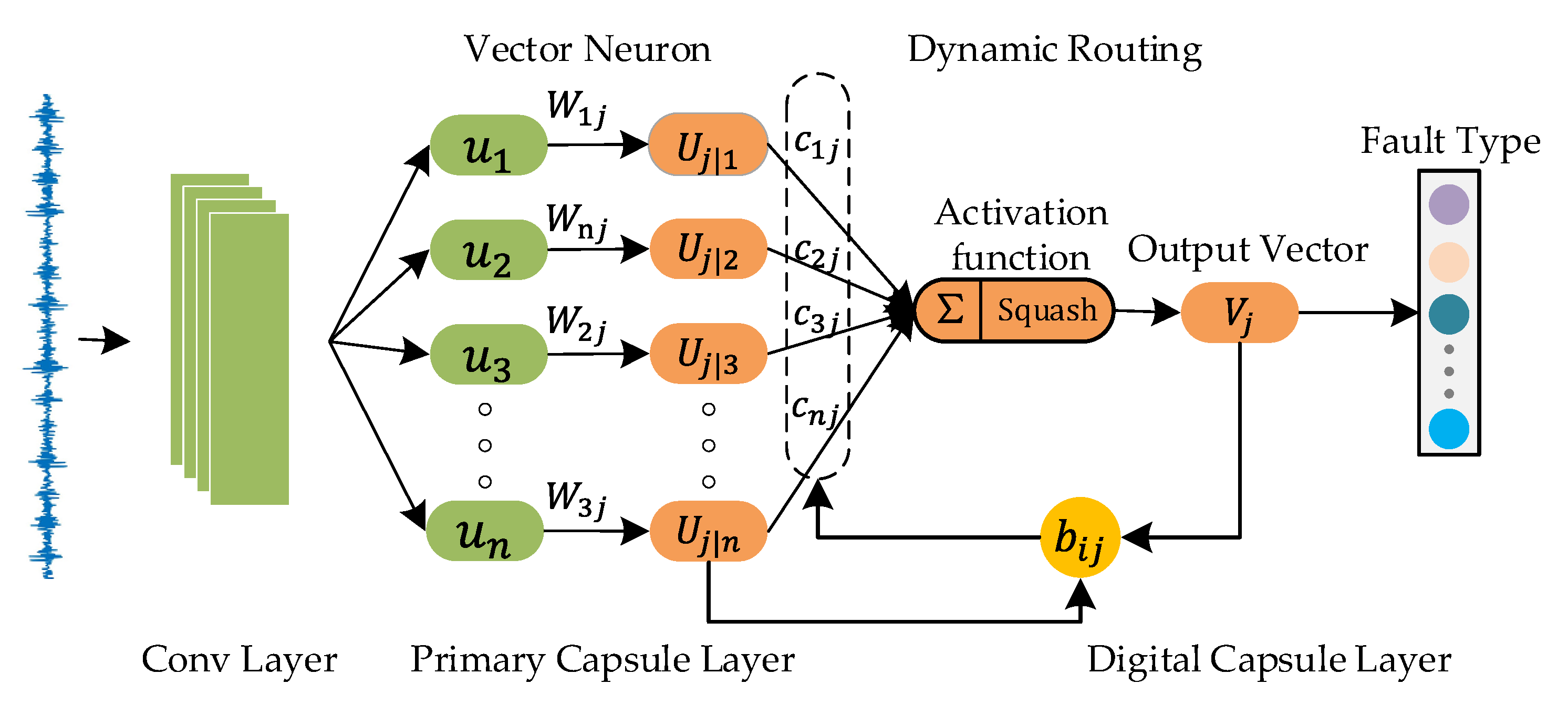
As shown in Figure 1, the capsule network is mainly composed of a convolution layer, primary capsule layer, and digital capsule layer. It is a high-performance neural network classifier that integrates feature extraction and pattern recognition.
Firstly, the model extracts the features of vibration signals through the convolution layer, and these features are used as the input data of the primary capsule layer. Secondly, the scalar neurons are transformed into vector neurons in the primary capsule layer, and the input feature scalar will also be reconstructed into feature vectors. The dynamic routing algorithm [26] can train the capsule network and measure their similarity through the dot products of capsule inputs and capsule outputs. It can transport low-level capsules to similar high-level capsules. So, a dynamic routing algorithm is used to train the connection weights between the primary capsule layer and digital capsule layer, and the output feature vectors are input into the digital capsule layer. Finally, the mold of the output vector in the digital capsule layer represents the probability of a certain fault type. The length of the vector represents fault types of the rolling bearing.
The operation process of capsule module can be divided into three steps.
First step, the product of the neuron and weight is expressed as a prediction vector , this process is shown below.
In the second step, the prediction vector is weighted, multiplied by the coupling coefficient (weight), and then summed to obtain the output vector . The weight is determined by the dynamic routing algorithm. The formula is as follows:
In a capsule network, the low-level capsules need to be delivered to the appropriate high-level capsules by a dynamic routing algorithm. The capsule network gathers the predicted close lower layers into a cluster in the higher layers . The biased forecasts will move away from the cluster. The weights are automatically adjusted by dynamic routing. stands for clustered cluster. The dynamic routing process is shown in Figure 2.
In the third step, the output vector obtains the final output through the nonlinear activation function, and the formula can be expressed as:
The calculation of the coupling coefficient is determined by . In the dynamic routing algorithm, are updated iteratively and then are adjusted, as shown in the equations.
where is initialized to 0, and the correlation is measured by the dot product of the vectors and . The positive dot product means that vectors multiply to a positive number. will increase as increases. On the contrary, the negative dot product is going to make go down. After cyclic iteration of the dynamic routing algorithm, a set of coupling coefficients of optimal matching between low-level capsules and high-level capsules are obtained.
3. Proposed Methodology
The capsule network can use vector neurons and a dynamic routing mechanism to capture fault feature information in the signal and mine the potential correlation between features. However, the traditional capsule network has only one convolution layer, and the convolution kernel scale is fixed. The extracted features are single. In a strong noise environment, the network is not sensitive to the periodic fault features of bearing vibration signals. Therefore, EIFN builds an enhanced integrated filter combining parallel way and cascaded way. It integrates feature extraction and noise filtering to improve the anti-noise capability of the model. The extracted scalar features are integrated into vector space, and the potential correlation between fault features of time-domain signals is mined.
3.1. Enhanced Integrated Filter
Section 2.1 shows that a one-dimensional convolution kernel can be used as a low-pass filter, which achieves better dynamic filtering. Then, we need to set the size of the one-dimensional convolution kernel. Short-time Fourier transform (STFT) divides the original time-domain signal into segments and adds windows on the basis of Fourier transform (FT) through a sliding window mechanism. It optimizes the problem that FT cannot handle the frequency component. For time-varying unsteady signals, the wide window is suitable for medium and low-frequency signals with high-frequency resolution. A narrow window is suitable for a high-frequency signal with high time resolution. Therefore, the enhanced integrated filter proposed in this paper uses a super-wide convolution kernel in the first layer to extract features and performs low-pass filtering of input signals. The super-wide convolution kernel pays more attention to the medium and low-frequency parts of the signal in the process of feature extraction to reduce the interference of high-frequency noise. The advantage of a super-wide convolution kernel is that it is obtained by an optimization algorithm, whereas the window function of STFT is an infinite length trig function. In summary, the super-wide convolution kernel automatically learns the features that are useful for fault diagnosis and automatically removes the features that interfere with diagnosis. It integrates feature extraction and low-pass filtering to improve the anti-noise capability of the model.
In the first layer, a single convolution with a super-wide kernel still has a similar problem to STFT. That is, a fixed window cannot ensure the resolution of frequency and time at the same time. Although wavelet transform can obtain frequency and time by changing the basis function, it is difficult to determine and change the wavelet basis function. We need to improve the single-layer super-wide kernel convolution. Based on experience, the first super-wide kernel convolution layer is set at the network entrance, and its kernel size is set to three times the step size [13]. Subsequently, three super-wide kernel convolution layers are added to the network entrance with successively increasing kernel size. Concatenate technology is used to connect four super-wide kernel convolution layers in parallel to achieve feature fusion in the channel dimension. Super-wide kernel convolution of diverse sizes can filter and retain different feature information in various visual fields. The fusion of extracted feature information can not only ensure time and frequency resolution to a certain extent but also reduce the interference of high-frequency noise by capturing the features of medium and low-frequency signals with super-wide windows. The convolution operation of parallel super-wide kernel convolutions on the original time-domain signal will intercept enough features. Further analysis of deep semantic features from fused features is another issue.
EIFN integrates multiple primary filters in parallel and cascaded modes to form the final strong filter, as shown in Figure 3.
Parallel super-wide kernel convolutions can effectively reduce noise, but the extracted feature information is extensive. If the model only cascades a single convolution layer, it is difficult to extract accurate signal features in each channel. Therefore, it is necessary to construct various small-scale convolutions to enhance feature expression, so as to highlight the features of the medium and low-frequency signals in the original signal.
3.2. The Architecture of EIFN
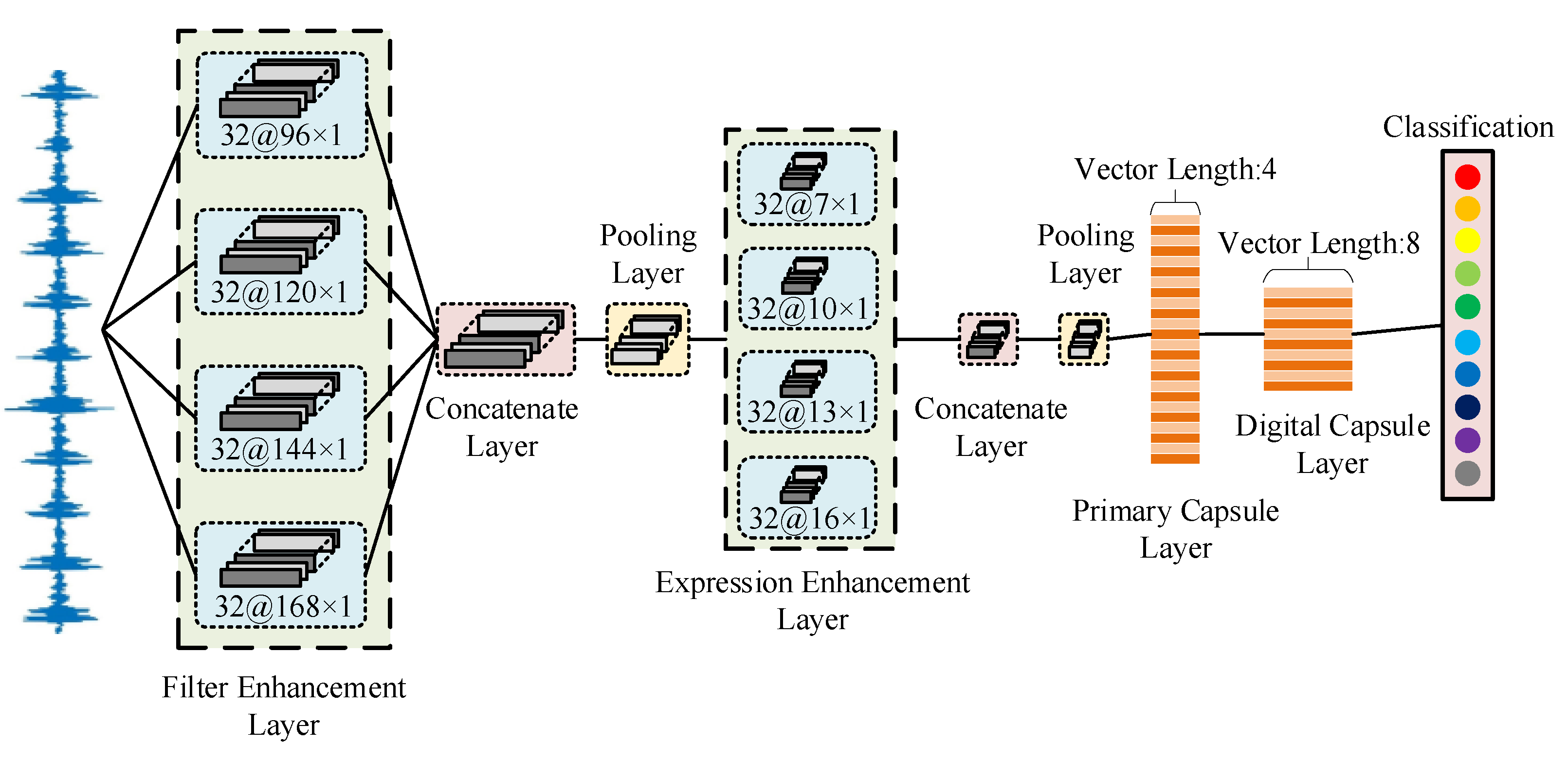
The model includes a filter enhancement layer, expression enhancement layer, concatenate layer, pooling layer, primary capsule layer, and digital capsule layer. The network structure of EIFN is shown in Figure 4.
EIFN firstly uses an enhanced integrated filter to perform noise filtering and feature extraction for the original vibration signal and then inputs to the primary capsule layer. The primary capsule layer reconstructs the input scalar feature layer into a vector neuron and transmits the feature in the way of dynamic routing. Finally, the length of the output vector of the digital capsule layer corresponds to different types of rolling bearing faults.
The filter enhancement layer in EIFN adopts four super-wide kernel convolutions of different scales to act on the original vibration signal. With different large receptive fields, it pays more attention to the useful signal features of middle and low frequencies and filters high-frequency noises to achieve multi-scale feature fusion. The expression enhancement layer uses various small convolution kernels to further extract features from the learning results of the upper layer. It can obtain better feature expression. The function of two pooling layers is to reduce the number of parameters, prevent overfitting, and optimize the network’s training speed. The leaky ReLU activation function is used for the filter enhancement layer, expression enhancement layer, and primary capsule layer. It can preserve the negative axis information in the feature vector, avoiding the constant zero neuron gradient. L2 regularization is also introduced.
The loss function is to measure the advantages and disadvantages of the model prediction. It describes the deviation between the model estimate and the observed value. During training, the model updated the weight to minimize the loss through the back propagation algorithm and optimized the weight in the process of continuous update and iteration. Since a capsule network allows multiple classifications to exist simultaneously, traditional cross-entropy cannot be used as the loss function in this paper. Therefore, interval loss is adopted, and the equation is as follows:
where stands for classification indicator function, c refers to classification number. Assuming that the correct label is 9, it can be considered that of the 9-th capsule is 1 and of other capsules is 0. is the mold length of the output vector and represents the classification probability. The upper bound is proposed and the value is set to 0.9. When is 0, the right-hand formula is calculated, and is 0.5 to ensure numerical stability of training. The lower bound is set to 0.1. The closer is to or , the smaller the loss value is. Square the formula to make the loss function conform to L2 regularization.
4. Experiments and Results
4.1. The Experimental Data
4.1.1. Case 1: CWRU Bearing Dataset
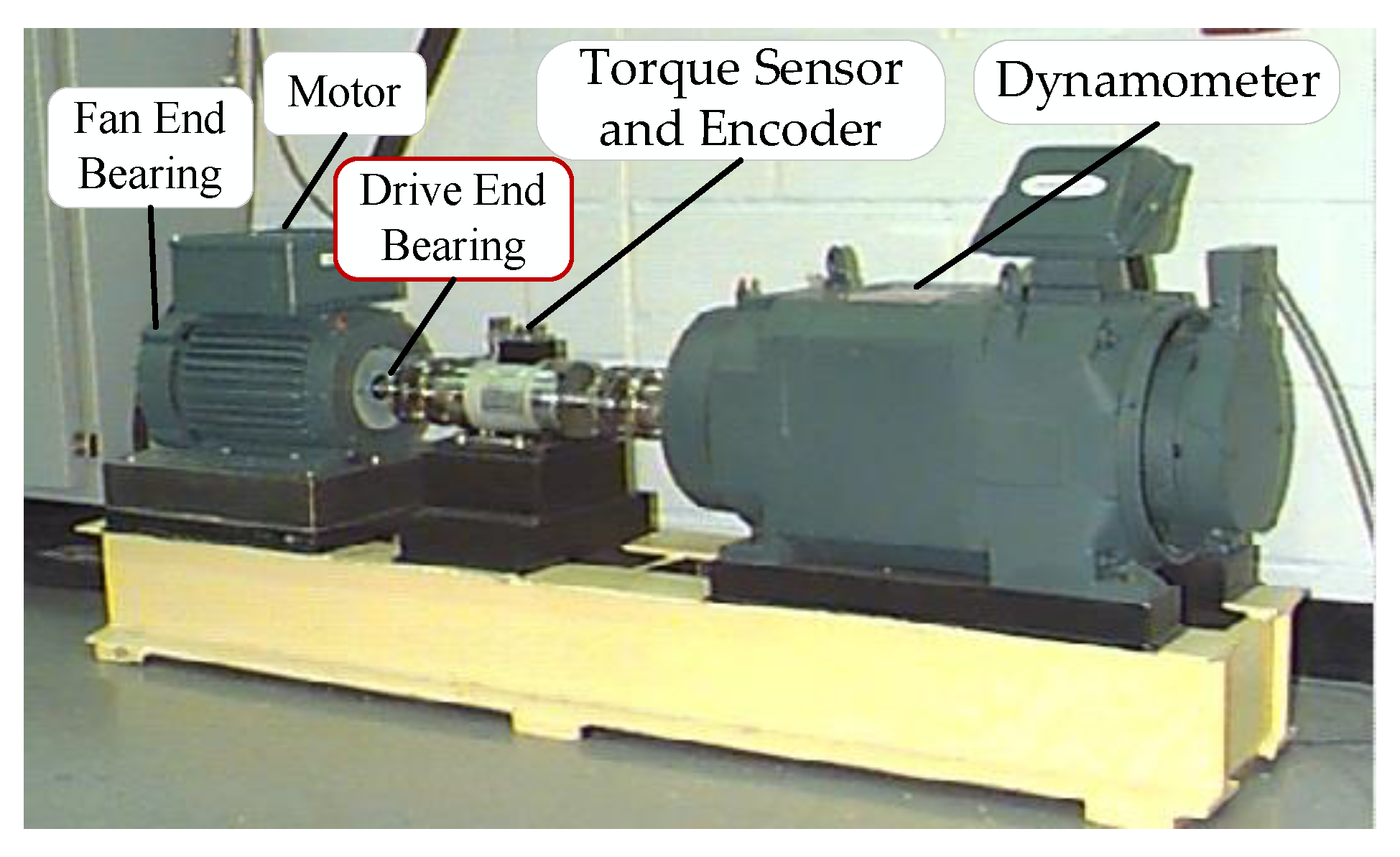
In this experiment, the bearing dataset of Case Western Reserve University is used as a benchmark. The bearing data acquisition system is shown in Figure 5.
The sampling frequency of the driving end bearing is 12 KHz. The bearing designation is SKF 6205-2RS. Single point damage is manufactured on the rolling ball, inner ring, and outer ring of the bearing by electric spark technology. The damage diameter is 0.007 inches, 0.014 inches, and 0.021 inches, respectively.
There are about 120,000 sample points for each fault data. Two thousand and forty-eight sample points are collected each time as a sample. The number of training samples that can be collected is limited. Therefore, data expansion is required. The method of data expansion is similar to the sliding window. One window contains 2048 sample points, which represents one sample. Each time 128 sample points are moved from the starting position, and the window of the new position is used as a new sample.
To ensure the integrity of signal features, we sequentially collected 2048 signal points to form a bearing state sample. In the CWRU dataset, each fault dataset has only 120,000 sampling points, and the amount of signal data is limited. Therefore, we use sliding window technology to expand the experimental data. As shown in Figure 6, the size of the sliding window is 2048, and the sliding step size (offset) is 128. Starting from the starting position, 128 sampling points are slid backward each time, and the sliding window collected 2048 sampling points to construct data samples in turn. Through data expansion, the construction of the sample library is completed. The process of data expansion is shown in Figure 6.
Samples at different speeds are selected to construct four groups of experimental data. The training set and testing set are divided into a 7:3 ratio. Dataset C1 are samples of 1772 rpm, C2 are samples of 1750 rpm, C3 are samples of 1720 RPM, and C4 are mixed samples of C1, C2, and C3. The dataset information is shown in Table 1.
Each dataset contains the samples of normal, ball fault, inner race fault, and outer race fault. The fault diameters are 0.007 inches, 0.014 inches, and 0.021 inches, respectively. Labels are made in one-hot encoding mode. One thousand samples are collected for each of the 10 types of data.
4.1.2. Case 2: IMS Bearing Dataset
The effectiveness of EIFN is further verified by using the IMS dataset, which is provided by the intelligent maintenance systems (IMS). The experimental platform is shown in Figure 7.
The speed of the four rolling bearings is 2000 rpm. They are subjected to a 6000 lbs radial load applied by the spring mechanism. The original signals are collected by vertical and horizontal accelerometers at a sampling frequency of 20 kHz. In order to be consistent with the CWRU experimental dataset, a fault status sample still contains 2048 sample points. The data expansion uses sliding window technology with a sliding step of 128. Ultimately, the dataset contains four states: normal, ball fault, inner race fault, and outer race fault. There are 1000 samples per bearing state. The training set and testing set are divided into a 7:3 ratio. The experimental dataset of IMS is shown in Table 2.
4.2. Model Parameters of EIFN
The filter enhancement layer is composed of four one-dimensional convolutions with scales of 96 × 1, 120 × 1, 144 × 1, and 168 × 1 in parallel. There are four one-dimensional convolution layers with scales of 7 × 1, 10 × 1, 13 × 1, and 16 × 1, which are connected in parallel to form the expression enhancement layer. The kernel sizes of the pooling layer are set to 2 × 1. The output of the second pooling layer is converted from feature scalar to feature vector by the primary capsule layer. The number of channels is 24. The dimension of the vector neuron is set as 4, and finally, the digital capsule layer outputs ten eight-dimensional vectors. With CWRU and IMS as datasets, the parameters of the model are essentially unchanged. The specific parameter settings are shown in Table 3. When the dataset is IMS, only the kernel size and output size of the digital capsule layer change to 4 and 4 × 8, respectively.
In the model training process, the epoch is set to 100 times and the batch size is set to 64. Adam optimizer is applied to the network and the initial learning rate is set to 0.001. Apply the learning rate decay strategy, which means a decrease of 10% after each iteration. Using dropout technology in the primary capsule layer to reduce overfitting and enhance the robustness.
4.3. Experimental Verification of EIFN’s Effectiveness
4.3.1. The Fault Diagnosis Result on CWRU Bearing Dataset
To verify the fault diagnosis effectiveness of EIFN, we use other models for comparison, such as SVM, DNN [12], wide-convolution deep convolutional neural network (WDCNN) [13], and series convolutional capsule network (SC-CAPSNET) [28]. As a general model, SVM combines with FFT and uses the radial basis function. The deep neural network here is FFT-DNN, which is a representative bearing fault diagnosis model. WDCNN is a classical convolutional neural network fault diagnosis method, which has certain anti-noise performance. SC-CAPSNET uses two single-scale convolution layers in series and simultaneously applies vector neurons and dynamic routing. In addition, the key modules of EIFN are ablated and replaced with conventional structures to explore the impact of each module on diagnostic performance. For example, the filter enhancement layer is replaced by a single-scale convolution with a kernel size of 127 × 1 (no FE). The expression enhancement layer is replaced by a single-scale convolution with a kernel size of 7 × 1 (no EE). The primary capsule layer and digital capsule layer are replaced by a convolution layer with a kernel size of 4 × 1, a flatten layer, and a dense layer (no vector).
In order to reduce the influence of random initialization, each model repeats the experiment five times on these datasets. We use the average of the five experimental results as the final result.
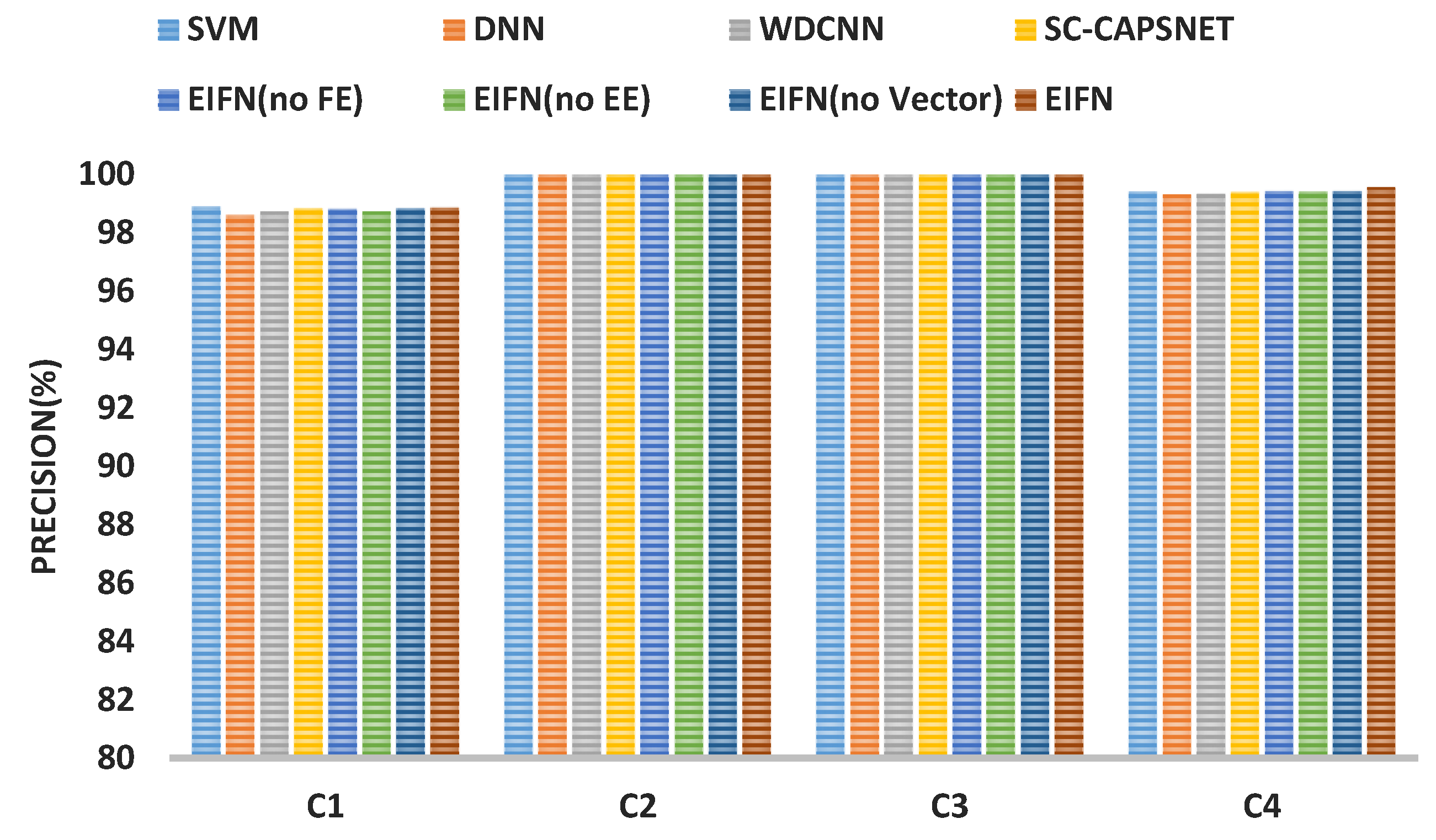
As shown in Figure 8, all models are tested on the four datasets (C1, C2, C3, C4). The fault diagnosis precisions of all models are about 99%, which shows that the intelligent fault diagnosis methods can correctly identify various bearing faults in a noise-free environment.
In order to increase the difference in fault diagnosis of various models, we added Gaussian white noise with SNR = 0 dB to the C1, C2, C3, and C4 datasets. All methods are evaluated with precision and recall. The fault diagnosis results are shown in Table 4.
In Table 4, the fault diagnosis precision and recall of SC-CAPSNET with vector neuron and dynamic routing on C1 and C4 are significantly better than that of WDCNN and SVM. The diagnostic results of the three models on C2 and C3 are relatively close. DNN has the worst performance, and the fault diagnosis precision on C2 and C3 is only about 78%. However, EIFN can still maintain more than 98% diagnostic precision on four datasets. The diagnostic precision and recall on C2 and C3 datasets with a lower rotation speed are also maintained at 100%. In addition, EIFN without key modules has good performance in fault diagnosis, but the precision and recall of fault diagnosis on the four datasets have been impaired to varying degrees. To sum up, the enhanced integrated filter, vector neuron, and dynamic routing all improve the noise resistance of the model to a certain extent and combine them to achieve the best results. The filter enhancement layer and expression enhancement layer of the enhanced integrated filter are indispensable.
The confusion matrixes for diagnostic accuracy of five models on dataset C4 are shown in Figure 9. From the diagram, it can be seen that performance differences of the five models are mainly reflected in the diagnostic accuracy of ball fault and outer race fault with a damage diameter of 0.014 inches (the labels are 2 and 8, respectively). DNN and WDCNN can hardly identify the two types of faults. The diagnostic performance of SC-CAPSNET is slightly better than that of SVM. However, EIFN can distinguish between the normal state and failure state samples correctly. The diagnostic accuracy of the inner race fault, outer race fault, and ball fault is basically 100%. The diagnostic accuracy is 94% only for detecting ball fault with a damage diameter of 0.014 inches. The experimental results show that EIFN can effectively extract fault features from the original signal and has a strong fault diagnosis ability.
4.3.2. The Fault Diagnosis Result on IMS Bearing Dataset
To increase the reliability of performance validation, the following experiments are performed using the IMS experimental dataset. White Gaussian noise is added to the testing set to make the SNR = 0 dB. We still use the above model for comparison. The average of the five experiment results is used as the final result. The models described in Section 4.3.1 are used to compare with EIFN. The fault diagnosis results are shown in Figure 10.
It can be seen from the diagram that the fault diagnosis performances and recall of the four EIFN models are all above 99%. SVM and SC-CAPSNET can reach more than the precision and recall of 97% in fault diagnosis precision, which is slightly better than SC-CAPSNET. The diagnosis precision of DNN is only 78% and susceptible to noise.
The confusion matrixes for diagnostic accuracy of the models are shown in Figure 11.
In Figure 11, EIFN achieves a recognition accuracy of 100% for the four states. SC-CAPSNET experiences a slight loss of accuracy in identifying the normal state with a label of 0. The diagnostic accuracy of SVM is slightly better than that of WDCNN. DNN has a greater loss of accuracy in identifying normal state and inner ring fault.
Based on the above experimental results, EIFN can still maintain a higher fault diagnosis accuracy compared with other models when subjected to low-intensity noise. The fault diagnosis performances of EIFN on CWRU and IMS datasets verified the validity of EIFN.
4.3.3. Visual Analysis of Feature Extraction Process
To explore the feature extraction process of EIFN, T-SNE technology is used to reduce the dimensionality of the features extracted from critical network layers of EIFN. The dataset used is the mixed dataset C4 of CWRU. Shown in Figure 12a–d is the two-dimensional distribution of extraction features in the filter enhancement layer, expression enhancement layer, primary capsule layer, and digital capsule layer.
In Figure 12, the same bearing state samples aggregation appears to a certain extent after the convolution operation of the original data in the filter enhancement layer. After the convolution operation of the expression enhancement layer, obvious bearing state classification has been shown, which fully demonstrates the feature expression ability of the expression enhancement layer. The feature expressions of the primary capsule layer and digital capsule layer show more significant classification features, and the feature expressions of the ten bearing states are clearly distinguishable. The above feature visualization effectively verified the rationality of the proposed method. EIFN improves the feature expression capability of the model by means of an enhanced integrated filter and transmits features in a dynamic routing mode combining with the features of vector neurons. It enables the model to produce distinguishing feature distributions more quickly. It also provides a basis for the model to detect signals with strong noise.
4.4. Comparative Analysis in Strong Noise Environment
4.4.1. Fault Diagnosis Results and Comparative Analysis
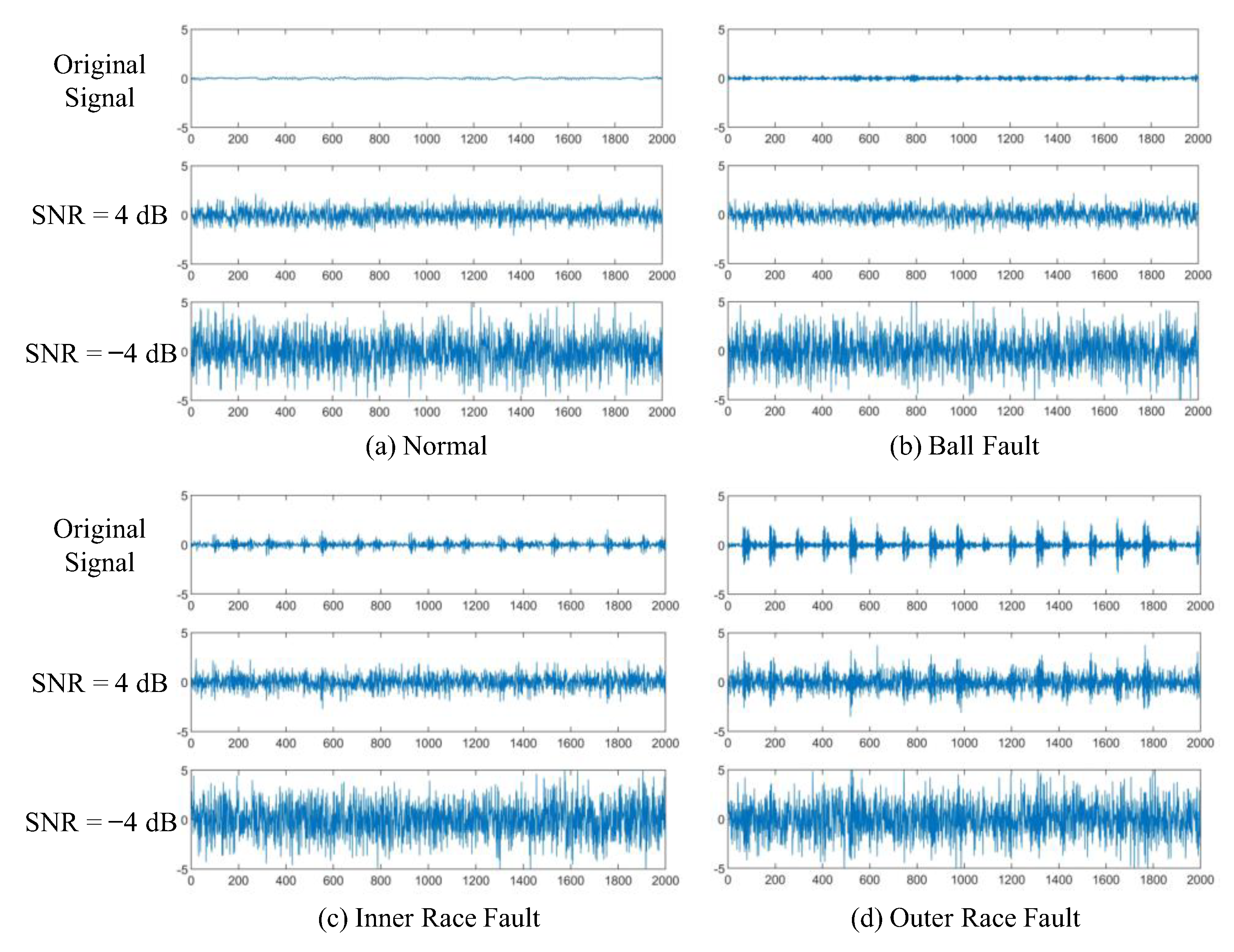
Gaussian white noise is added to the normal and fault state signals of rolling bearings, and SNR = 4 dB, −4 dB. The smaller the SNR, the stronger the noise is. The signal waveforms are shown in Figure 13.
In Figure 13, Figure 13a is the bearing vibration signal in the normal state, and Figure 13b–d are the signals of ball, inner race, and outer race with a fault diameter of 0.007 inches, respectively. The amplitudes of original signals in four states show periodic changes with obvious regularity. In the signal with SNR = 4 dB, the types of normal state, ball fault, and inner race fault could not be distinguished. The signal features of the outer race fault state are partially submerged by noise, but the fault type could still be distinguished. In the signal with SNR = −4 dB, signal vibration features of four states are completely submerged by noise. The fault types of signals with low SNR cannot be directly identified. Therefore, the difficulty of rolling bearing fault diagnosis increases greatly in a strong noise environment.
In order to verify the fault diagnosis performance of EIFN in a strong noise environment, Gaussian white noise with different SNR is added to the test dataset of C4 on CWRU and the test dataset on IMS. The comparative experiment is conducted with SVM, DNN, WDCNN, SC-CAPSNET, and EIFN (no key module). Experimental results are shown in Table 5 and Table 6 and Figure 14.
In Table 5 and Figure 14a, the fault diagnosis precision and recall of SVM, WDCNN, and SC-CAPSNET are around 90% in the environment with weak noise of 0–4 dB, while that of EIFN is above 99%. The fault diagnosis precision of DNN can only achieve 85% even in the noise environment with SNR = 4 dB. With the increase in noise intensity, the fault diagnosis precision of SVM, DNN, WDCNN, and SC-CAPSNET decreases obviously. When SNR is −2 dB, the diagnosis precision of the EIFN model remains at 98.33%, while that of SC-CAPSNET is only 83.78%. The diagnostic precision and recall of SVM, DNN, and WDCNN are all below 74%. In the strong noise environment with SNR = −4 dB, EIFN still maintains a bearing fault classification recognition precision of 94.73%, while that of SC-CAPSNET is only 71.63%. The fault diagnosis precision and recall of SVM, DNN, and WDCNN are all below 59%. We can find that SVM and WDCNN can achieve high fault diagnosis precision in a low-noise environment, but it is seriously disturbed in high-intensity noise. DNN has poor fault diagnosis performance in a noisy environment. The three types of EIFN without key modules have similar diagnostic performance. In the strong noise environment, the fault diagnosis accuracies of the three models are better than SVM, DNN, WDCNN, and SC-CAPSNET, but the diagnosis performances are lower than EIFN. Three key modules have improved the noise resistance of the model, and the best effect can be achieved by integrating three modules.
In Table 6 and Figure 14b, we can find that other models except DNN have a similar fault diagnosis performance when SNR = 0 dB − 4 dB. When SNR is −4 dB, the fault diagnosis precision and recall of SVM, DNN, and WDCNN decrease greatly. Compared with SVM, SC-CAPSNET has less degradation in fault diagnosis performance, highlighting the advantages of vector neurons. In addition, the diagnostic precision of the three types of EIFN without key modules also declined significantly compared with the results on the CWRU dataset. However, EIFN can still achieve 92.45% fault diagnosis precision without much interference.
4.4.2. Discussion on Experimental Results
In Figure 13, the original signal can be represented as the data in the training set, and the signal with SNR = −4 dB can be represented as the data in the test set. The periodic shock features of the testing set with noise are entirely submerged, which is quite different from the training set without noise. It can be seen from Figure 8 that most models can achieve high fault diagnosis precision with no noise. At this point, the training set and the testing set are the same dataset. In Figure 14, when Gaussian white noise is added to the testing set to make SNR = −4 dB, the bearing fault diagnosis precision of SVM, DNN, WDCNN, and SC-CAPSNET is less than 72%. At this point, the diversity of the training set and testing set is large. The models trained by the above method using the training set cannot achieve good results on the unknown dataset (the testing set), and the generalization abilities are weak. However, EIFN can achieve more than 92% fault diagnosis precision on both CWRU and IMS datasets. This shows that EIFN has a strong generalization ability and has good fault diagnosis performance for both the known training set and unknown testing set.
4.4.3. Feature Visualization Analysis
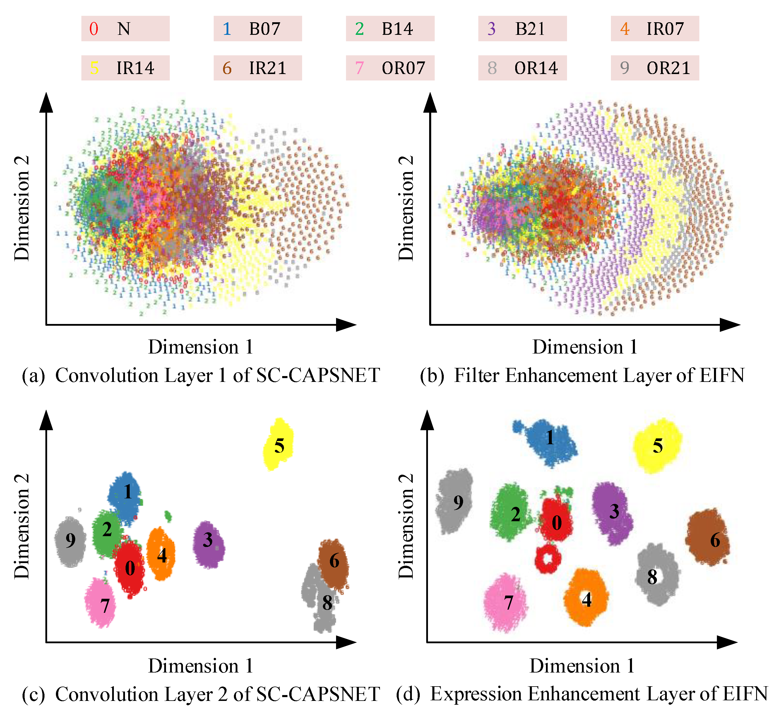
In order to explore the extraction process of bearing fault feature information by EIFN in a strong noise environment, Gaussian white noise is added to the mixed dataset C4 in CWRU to make the SNR = −4 dB. T-SNE technology is used to visualize the features extracted from the filter enhancement layer and the expression enhancement layer of EIFN, and the results are compared with two serial convolution layers of SC-CAPSNET, as shown in Figure 15.
In Figure 15, Figure 15a is the extraction feature of SC-CAPSNET’s first convolution layer to the original vibration signal, and Figure 15b is the extraction feature of EIFN’s filter enhancement layer to the original vibration signal. In Figure 15b, B21, IR14, and IR21 have clearly presented a crescent-shaped aggregation effect. While in Figure 15a, only IR14 and IR21 have clustering and have more intersections and overlaps with other categories. Figure 15c,d are the features extracted from the second convolution layer of SC-CAPSNET and the expression enhancement layer of EIFN, respectively. In Figure 15d, EIFN’s expression enhancement layer has clearly distinguished other fault categories except N and B14. However, N, B07, B14, IR21, and OR14 in the features extracted by the second convolution layer of SC-CAPSNET all converge. In summary, EIFN constructs an enhanced integrated filter by cascading a filter enhancement layer, expression enhancement layer, and sampling layers. The structure uses multi-scale filters to extract features and filter noise of the original vibration signal with different visual fields, highlighting the key information of fault features. Features in each field complement each other to highlight key information of fault features. The visualization results show that the enhanced integrated filter can maintain excellent feature extraction capability even when disturbed by strong noise.
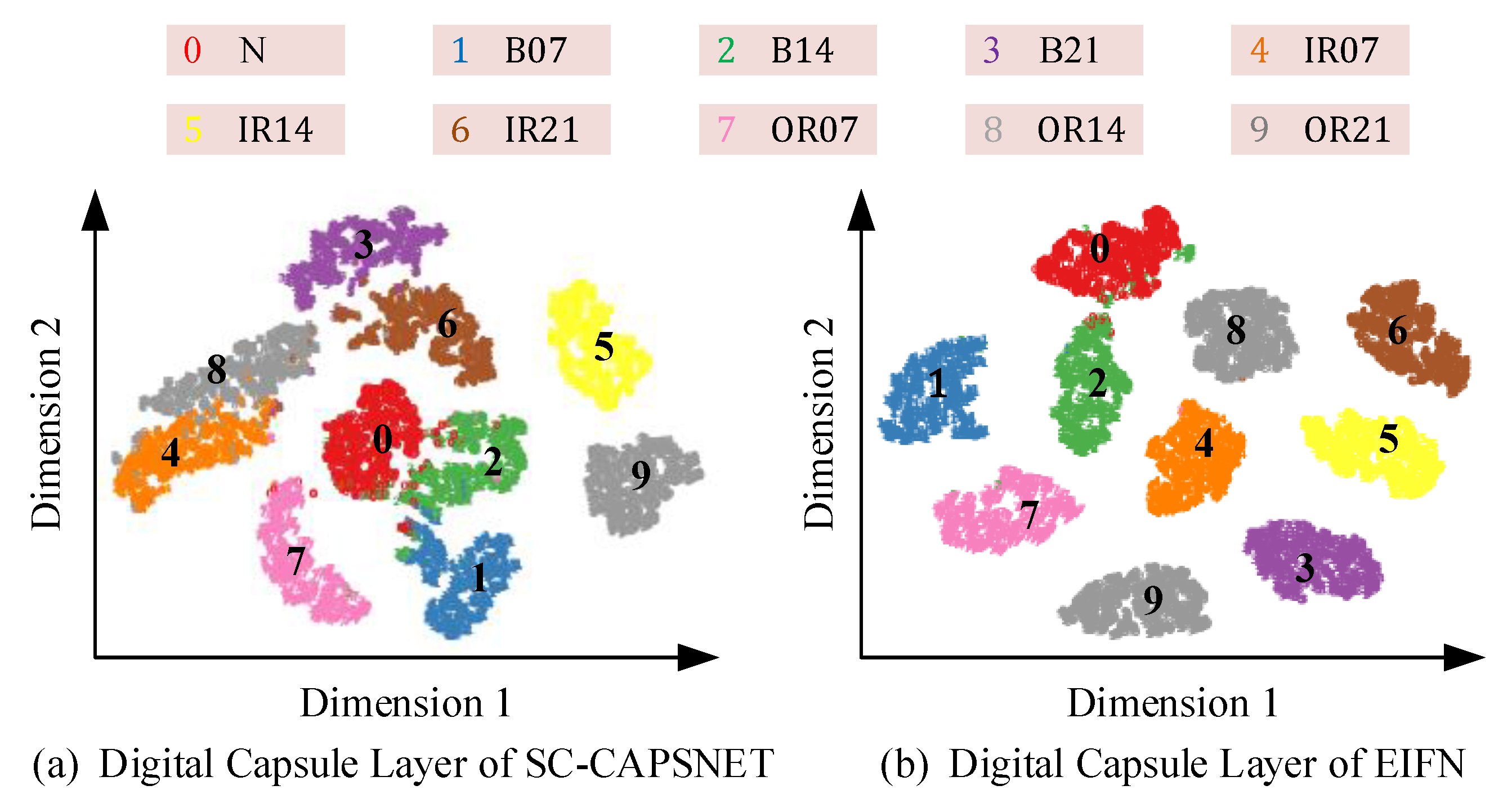
As shown in Figure 16, the model classification results of the digital capsule layer (full connection layer) of EIFN and SC-CAPSNET are visualized.
In Figure 16a, after feature visualization in SC-CAPSNET’s digital capsule layer, IR07 and OR14 are confused, B21 and IR21 converge, and N overlaps with B14 and B07. Obviously, when SC-CAPSNET detects vibration signals with low SNR, the classification effect of the rolling bearing fault state is not ideal. It is difficult to distinguish normal states and various faults. In Figure 16b, ten data samples in the digital capsule layer of EIFN are obviously clustered into ten clusters. Only a small part of the fault state of the ball labeled 2 intersected with the normal state of the bearing labeled 0. Other clusters have a large degree of differentiation. The visualization results highlight the advantages of the enhanced filter combined with vector neurons. The filtered features are integrated into vector space and then transferred in dynamic routing. The feature expression of the model is more explicit, and the interference of strong noise is reduced effectively.
5. Conclusions
The paper proposes EIFN, which integrates feature extraction and signal filtering by constructing an enhanced integrated filter set. The feature scalar filtered by the filter is transformed into a feature vector and transmitted by a dynamic route. The combination of the two aspects improves the fault diagnosis precision of the model in a strong noise environment.
- (1)
- EIFN integrates multiple primary filters in parallel and cascaded mode to form the enhanced integrated filter. It can not only filter high-frequency noise and extract useful feature information of low and middle frequency but also maintain frequency and time resolution to a certain extent.
- (2)
- EIFN uses vector neurons to incorporate scalar feature information into vector spaces. The relationship between low-level features and high-level features is established by dynamic routing. The key information of multi-scale fault features of signal in the time dimension is highlighted to improve the precision of bearing fault diagnosis in a strong noise environment.
- (3)
- The experimental results show that EIFN can effectively identify various types of rolling bearing states, and the bearing fault diagnosis precisions are more than 92% when strong noise of SNR = −4 dB. The visualization results verify that EIFN can effectively extract low and medium-frequency feature information and filter high-frequency noise through the enhanced integrated filter.
Author Contributions
K.W. conceptualization, methodology, software, visualization, writing—original draft, investigation; J.T. supervision, data curation, writing—review and editing, validation, investigation, funding acquisition; D.Y. writing—review and editing, methodology; H.X. software, resources; Z.L. software, resources. All authors have read and agreed to the published version of the manuscript.
Funding
This research is funded by the National Natural Science Foundation of China (Grant No. 51875199), the National Natural Science Foundation of Hunan Province (Grant No. 2021JJ30267, No. 2019JJ50156) and the Excellent youth fund of Hunan Provincial Department of Education (Grant No. 19B187, No. 21B0484).
Institutional Review Board Statement
Not applicable.
Informed Consent Statement
Not applicable.
Data Availability Statement
Not applicable.
Conflicts of Interest
The authors declare no conflict of interest.
References
- Hoang, D.T.; Kang, H.J. A survey on Deep Learning based bearing fault diagnosis. Neurocomputing 2019, 335, 327–335. [Google Scholar] [CrossRef]
- Xia, M.; Li, T.; Xu, L.; Liu, L.; De Silva, C.W. Fault diagnosis for rotating machinery using multiple sensors and convolutional neural networks. IEEE/ASME Trans. Mechatron. 2017, 23, 101–110. [Google Scholar] [CrossRef]
- El-Thalji, I.; Jantunen, E. A summary of fault modelling and predictive health monitoring of rolling element bearings. Mech. Syst. Signal Process. 2015, 60, 252–272. [Google Scholar] [CrossRef]
- Yan, X.; She, D.; Xu, Y.; Jia, M. Deep regularized variational autoencoder for intelligent fault diagnosis of rotor–bearing system within entire life-cycle process. Knowl. Based Syst. 2021, 226, 107142. [Google Scholar] [CrossRef]
- Li, G.; Tang, G.; Luo, G.; Wang, H. Underdetermined blind separation of bearing faults in hyperplane space with variational mode decomposition. Mech. Syst. Signal Process. 2019, 120, 83–97. [Google Scholar] [CrossRef]
- Qin, C.; Wang, D.; Xu, Z.; Tang, G. Improved empirical wavelet transform for compound weak bearing fault diagnosis with acoustic signals. Appl. Sci. 2020, 10, 682. [Google Scholar] [CrossRef] [Green Version]
- Cheng, Y.; Wang, Z.; Chen, B.; Zhang, W.; Huang, G. An improved complementary ensemble empirical mode decomposition with adaptive noise and its application to rolling element bearing fault diagnosis. ISA Trans. 2019, 91, 218–234. [Google Scholar] [CrossRef]
- Li, X.; Yang, Y.; Pan, H.; Cheng, J.; Cheng, J. A novel deep stacking least squares support vector machine for rolling bearing fault diagnosis. Comput. Ind. 2019, 110, 36–47. [Google Scholar] [CrossRef]
- Gunerkar, R.S.; Jalan, A.K.; Belgamwar, S.U. Fault diagnosis of rolling element bearing based on artificial neural network. J. Mech. Sci. Technol. 2019, 33, 505–511. [Google Scholar] [CrossRef]
- Zhang, N.; Wu, L.; Yang, J.; Guan, Y. Naive bayes bearing fault diagnosis based on enhanced independence of data. Sensors 2018, 18, 463. [Google Scholar] [CrossRef] [Green Version]
- Zhang, S.; Zhang, S.; Wang, B.; Habetler, T.G. Deep learning algorithms for bearing fault diagnostics—A comprehensive review. IEEE Access 2020, 8, 29857–29881. [Google Scholar] [CrossRef]
- Jia, F.; Lei, Y.; Lin, J.; Zhou, X.; Lu, N. Deep neural networks: A promising tool for fault characteristic mining and intelligent diagnosis of rotating machinery with massive data. Case Stud. Mech. Syst. Signal Process. 2016, 72, 303–315. [Google Scholar] [CrossRef]
- Zhang, W.; Peng, G.; Li, C.; Chen, Y.; Zhang, Z. A new deep learning model for fault diagnosis with good anti-noise and domain adaptation ability on raw vibration signals. Sensors 2017, 17, 425. [Google Scholar] [CrossRef]
- Eren, L.; Ince, T.; Kiranyaz, S. A generic intelligent bearing fault diagnosis system using compact adaptive 1D CNN classifier. J. Signal Process Syst. 2019, 91, 179–189. [Google Scholar] [CrossRef]
- Han, T.; Zhang, L.; Yin, Z.; Tan, A.C. Rolling bearing fault diagnosis with combined convolutional neural networks and support vector machine. Measurement 2021, 177, 109022. [Google Scholar] [CrossRef]
- Li, X.; Jiang, H.; Zhao, K.; Wang, R. A deep transfer nonnegativity-constraint sparse autoencoder for rolling bearing fault diagnosis with few labeled data. IEEE Access 2019, 7, 91216–91224. [Google Scholar] [CrossRef]
- Zhao, K.; Jiang, H.; Li, X.; Wang, R. An optimal deep sparse autoencoder with gated recurrent unit for rolling bearing fault diagnosis. Meas. Sci. Technol. 2019, 31, 015005. [Google Scholar] [CrossRef]
- Wu, Z.; Jiang, H.; Zhao, K.; Li, X. An adaptive deep transfer learning method for bearing fault diagnosis. Measurement 2020, 151, 107227. [Google Scholar] [CrossRef]
- Zou, Y.; Liu, Y.; Deng, J.; Jiang, Y.; Zhang, W. A novel transfer learning method for bearing fault diagnosis under different working conditions. Measurement 2021, 171, 108767. [Google Scholar] [CrossRef]
- Wang, Y.; Cheng, L. A combination of residual and long–short-term memory networks for bearing fault diagnosis based on time-series model analysis. Meas. Sci. Technol. 2020, 32, 015904. [Google Scholar] [CrossRef]
- Hao, S.; Ge, F.X.; Li, Y.; Jiang, J. Multisensor bearing fault diagnosis based on one-dimensional convolutional long short-term memory networks. Measurement 2020, 159, 107802. [Google Scholar] [CrossRef]
- Zhang, Z.; Li, H.; Chen, L.; Han, P. Rolling bearing fault diagnosis using improved deep residual shrinkage networks. Shock. Vib. 2021, 2021, 9942249. [Google Scholar] [CrossRef]
- Tong, Y.; Wu, P.; He, J.; Zhang, X.; Zhao, X. Bearing fault diagnosis by combining a deep residual shrinkage network and bidirectional LSTM. Meas. Sci. Technol. 2021, 33, 034001. [Google Scholar] [CrossRef]
- Chen, Z.; Mauricio, A.; Li, W.; Gryllias, K. A deep learning method for bearing fault diagnosis based on cyclic spectral coherence and convolutional neural networks. Mech. Syst. Signal Process. 2020, 140, 106683. [Google Scholar] [CrossRef]
- Xu, Z.; Li, C.; Yang, Y. Fault diagnosis of rolling bearing of wind turbines based on the variational mode decomposition and deep convolutional neural networks. Appl. Soft Comput. 2020, 95, 106515. [Google Scholar] [CrossRef]
- Sabour, S.; Frosst, N.; Hinton, G.E. Dynamic routing between capsules. In Proceedings of the 31st Conference on Neural Information Processing Systems (NIPS), Long Beach, CA, USA, 4–9 December 2017; pp. 3859–3869. [Google Scholar]
- Chen, T.; Wang, Z.; Yang, X.; Jiang, K. A deep capsule neural network with stochastic delta rule for bearing fault diagnosis on raw vibration signals. Measurement 2019, 148, 106857. [Google Scholar] [CrossRef]
- Yang, P.; Su, Y.C.; Zhang, Z. A study on rolling bearing fault diagnosis based on convolution capsule network. J. Vib. Shock 2020, 39, 55–62+68. [Google Scholar]
- Huang, R.; Li, J.; Wang, S.; Li, G.; Li, W. A robust weight-shared capsule network for intelligent machinery fault diagnosis. IEEE Trans. Ind. Inform. 2020, 16, 6466–6475. [Google Scholar] [CrossRef]
- Han, T.; Ma, R.; Zheng, J. Combination bidirectional long short-term memory and capsule network for rotating machinery fault diagnosis. Measurement 2021, 176, 109208. [Google Scholar] [CrossRef]
- Li, L.; Zhang, M.; Wang, K. A fault diagnostic scheme based on capsule network for rolling bearing under different rotational speeds. Sensors 2020, 20, 1841. [Google Scholar] [CrossRef] [Green Version]
- Zhu, Z.; Peng, G.; Chen, Y.; Gao, H. A convolutional neural network based on a capsule network with strong generalization for bearing fault diagnosis. Neurocomputing 2019, 323, 62–75. [Google Scholar] [CrossRef]
- Sun, Z.; Yuan, X.; Fu, X.; Zhou, F.; Zhang, C. Multi-Scale Capsule Attention Network and Joint Distributed Optimal Transport for Bearing Fault Diagnosis under Different Working Loads. Sensors 2021, 21, 6696. [Google Scholar] [CrossRef]
- Wang, Z.; Zheng, L.; Du, W.; Cai, W.; Zhou, J.; Wang, J.; He, G. A novel method for intelligent fault diagnosis of bearing based on capsule neural network. Complexity 2019, 2019, 6943234. [Google Scholar] [CrossRef] [Green Version]
- Wang, Y.; Ning, D.; Feng, S. A novel capsule network based on wide convolution and multi-scale convolution for fault diagnosis. Appl. Sci. 2020, 10, 3659. [Google Scholar] [CrossRef]
- Li, Y.; Wang, N.; Shi, J.; Liu, J.; Hou, X. Revisiting Batch Normalization for Practical Domain Adaptation. arXiv 2016, arXiv:1603.04779. [Google Scholar]
Figure 1.
The architecture of a capsule network. The transformation of scalar neurons into vector neurons occurs in the primary capsule layer. Dynamic routing occurs between the primary capsule layer and the digital capsule layer.
Figure 1.
The architecture of a capsule network. The transformation of scalar neurons into vector neurons occurs in the primary capsule layer. Dynamic routing occurs between the primary capsule layer and the digital capsule layer.

Figure 2.
The dynamic routing of the capsule network.

Figure 3.
The structure of the enhanced integrated filter. K × 1 represents the sizes of the convolution kernel. Concatenate stands for feature fusion. Sampling represents using the pooling layer.
Figure 3.
The structure of the enhanced integrated filter. K × 1 represents the sizes of the convolution kernel. Concatenate stands for feature fusion. Sampling represents using the pooling layer.

Figure 4.
The structure of EIFN. The part in front of @ represents the number of channels, and the part behind @ indicates the size of the convolution kernel. See Section 4.2 for specific parameters.
Figure 4.
The structure of EIFN. The part in front of @ represents the number of channels, and the part behind @ indicates the size of the convolution kernel. See Section 4.2 for specific parameters.

Figure 5.
The bearing data acquisition device. From left to right are fan end bearing, motor, drive end bearing, torque sensor and encoder, and dynamometer. The place marked in the red box is the drive end bearing we need to use.
Figure 5.
The bearing data acquisition device. From left to right are fan end bearing, motor, drive end bearing, torque sensor and encoder, and dynamometer. The place marked in the red box is the drive end bearing we need to use.

Figure 6.
The process of data expansion. Offset is the sliding distance of the window, representing 128 sample points. Overlap is the repeated part of two adjacent windows after sliding. Width of gathering is 2048 sample points.
Figure 6.
The process of data expansion. Offset is the sliding distance of the window, representing 128 sample points. Overlap is the repeated part of two adjacent windows after sliding. Width of gathering is 2048 sample points.

Figure 7.
Experimental platform of IMS. The platform mainly consists of four Rexnord za-2115 double row bearings, thermocouples, an AC motor (at 2000 rpm), and vibration sensors (x-axis and y-axis).
Figure 7.
Experimental platform of IMS. The platform mainly consists of four Rexnord za-2115 double row bearings, thermocouples, an AC motor (at 2000 rpm), and vibration sensors (x-axis and y-axis).

Figure 8.
The result of bearing fault diagnosis on CWRU without noise. The abscissa is the dataset, and the ordinate is the precision of fault diagnosis.
Figure 8.
The result of bearing fault diagnosis on CWRU without noise. The abscissa is the dataset, and the ordinate is the precision of fault diagnosis.

Figure 9.
The confusion matrix of diagnostic accuracy on CWRU. The abscissa is the prediction label, and the ordinate is the real label.
Figure 9.
The confusion matrix of diagnostic accuracy on CWRU. The abscissa is the prediction label, and the ordinate is the real label.

Figure 10.
The result of bearing fault diagnosis on IMS. The figure contains two indicators: precision and recall.
Figure 10.
The result of bearing fault diagnosis on IMS. The figure contains two indicators: precision and recall.

Figure 11.
The confusion matrix of diagnostic accuracy on IMS. The abscissa is the prediction label, and the ordinate is the real label.
Figure 11.
The confusion matrix of diagnostic accuracy on IMS. The abscissa is the prediction label, and the ordinate is the real label.

Figure 12.
The visualization of the feature extraction process in EIFN. Here, 0–9 are labels for bearing status, where N represents normal state, B, IR, and OR represent ball, inner race, and outer race faults, respectively. The numbers represent fault diameters.
Figure 12.
The visualization of the feature extraction process in EIFN. Here, 0–9 are labels for bearing status, where N represents normal state, B, IR, and OR represent ball, inner race, and outer race faults, respectively. The numbers represent fault diameters.

Figure 13.
Original signal, the mixed signal with SNR = 4 dB, and the mixed signal with SNR = −4 dB in different fault state. The abscissa is the number of samples, and the ordinate is the amplitude.
Figure 13.
Original signal, the mixed signal with SNR = 4 dB, and the mixed signal with SNR = −4 dB in different fault state. The abscissa is the number of samples, and the ordinate is the amplitude.

Figure 14.
The comparison of diagnostic precision in different SNR noise environment. The abscissa is the SNR, and the ordinate is the fault diagnosis precision.
Figure 14.
The comparison of diagnostic precision in different SNR noise environment. The abscissa is the SNR, and the ordinate is the fault diagnosis precision.

Figure 15.
The feature visualization. Here, 0–9 indicates different bearing states.

Figure 16.
The feature visualization of digital capsule layer.


Table 1.
The experimental dataset of CWRU.
| Fault Label | Fault Category | Fault Diameter | Sample Size |
|---|---|---|---|
| 0 | Normal | 0 | 1000 |
| 1 | Ball fault | 0.007 | 1000 |
| 2 | Ball fault | 0.014 | 1000 |
| 3 | Ball fault | 0.021 | 1000 |
| 4 | Inner race fault | 0.007 | 1000 |
| 5 | Inner race fault | 0.014 | 1000 |
| 6 | Inner race fault | 0.021 | 1000 |
| 7 | Outer race fault | 0.007 | 1000 |
| 8 | Outer race fault | 0.014 | 1000 |
| 9 | Outer race fault | 0.021 | 1000 |
Table 2.
The experimental dataset of IMS.
| Fault Label | Fault Category | Training Set | Testing Set |
|---|---|---|---|
| 0 | Normal | 700 | 300 |
| 1 | Inner race fault | 700 | 300 |
| 2 | Ball fault | 700 | 300 |
| 3 | Outer race fault | 700 | 300 |
Table 3.
The network parameters of EIFN.
| Layer Type | Operation | Kernel Size | Stride | Kernel Number | Output Size | Parallel Output Size | Padding |
|---|---|---|---|---|---|---|---|
| Filter enhancement layer | Convolution 1 | 96 × 1 | 32 | 32 | 64 × 32 | 64 × 128 | Yes |
| Convolution 2 | 120 × 1 | 32 | 32 | 64 × 32 | Yes | ||
| Convolution 3 | 144 × 1 | 32 | 32 | 64 × 32 | Yes | ||
| Convolution 4 | 168 × 1 | 32 | 32 | 64 × 32 | Yes | ||
| Pooling layer | Sampling | 2 × 1 | 2 | 32 | 32 × 128 | No | |
| Expression enhancement layer | Convolution 1 | 7 × 1 | 2 | 32 | 16 × 32 | 16 × 128 | Yes |
| Convolution 2 | 10 × 1 | 2 | 32 | 16 × 32 | Yes | ||
| Convolution 3 | 13 × 1 | 2 | 32 | 16 × 32 | Yes | ||
| Convolution 4 | 16 × 1 | 2 | 32 | 16 × 32 | Yes | ||
| Pooling layer | Sampling | 2 × 1 | 2 | 32 | 8 × 128 | No | |
| Primary capsule layer | Construct of vector neurons | 4 × 1 | 2 | 32 | 24 × 4 | No | |
| Digital capsule layer | Dynamic routing | 10/4 | 1 | 10 × 8/4 × 8 | No |
Table 4.
Fault diagnosis precision (%) and recall (%) of models.
| Model | C1 | C2 | C3 | C4 | ||||
|---|---|---|---|---|---|---|---|---|
| Precision | Recall | Precision | Recall | Precision | Recall | Precision | Recall | |
| SVM | 91.43 | 92.07 | 97.08 | 97.21 | 98.74 | 99.12 | 86.23 | 87.16 |
| DNN | 65.11 | 64.52 | 77.63 | 77.81 | 78.28 | 79.34 | 57.89 | 58.74 |
| WDCNN | 86.24 | 86.01 | 96.71 | 96.76 | 96.13 | 95.01 | 81.92 | 82.34 |
| SC-CAPSNET | 95.87 | 96.21 | 97.13 | 97.64 | 99.48 | 99.56 | 92.54 | 93.23 |
| EIFN (no FE) | 97.21 | 97.38 | 98.73 | 99.91 | 99.72 | 99.78 | 98.71 | 98.83 |
| EIFN (no EE) | 96.74 | 96.91 | 98.97 | 99.83 | 99.87 | 99.91 | 97.91 | 98.23 |
| EIFN (no Vector) | 96.56 | 96.73 | 99.76 | 99.92 | 100 | 100 | 98.54 | 98.62 |
| EIFN | 98.73 | 99.21 | 100 | 100 | 100 | 100 | 99.18 | 99.23 |
Table 5.
Fault diagnosis results on CWRU.
| Model | −4 dB | −2 dB | 0 dB | 2 dB | 4 dB | |||||
|---|---|---|---|---|---|---|---|---|---|---|
| Precision | Recall | Precision | Recall | Precision | Recall | Precision | Recall | Precision | Recall | |
| SVM | 58.31 | 57.56 | 72.97 | 73.43 | 86.23 | 87.16 | 94.52 | 95.87 | 99.11 | 98.79 |
| DNN | 42.37 | 41.28 | 49.92 | 50.62 | 57.89 | 58.74 | 70.62 | 70.88 | 85.63 | 86.35 |
| WDCNN | 57.45 | 56.78 | 67.38 | 66.94 | 81.92 | 82.34 | 86.21 | 85.75 | 96.81 | 97.03 |
| SC-CAPSNET | 71.63 | 72.01 | 83.78 | 84.25 | 92.54 | 93.23 | 95.97 | 96.71 | 98.41 | 98.56 |
| EIFN (no FE) | 88.76 | 88,63 | 95.91 | 95.77 | 98.71 | 98.83 | 99.23 | 99.14 | 99.33 | 99.36 |
| EIFN (no EE) | 86.84 | 87.72 | 96.11 | 96.71 | 97.91 | 98.23 | 99.19 | 99.15 | 99.38 | 99.32 |
| EIFN (no Vector) | 87.21 | 88.19 | 96.22 | 96.81 | 98.54 | 98.62 | 99.18 | 99.21 | 99.42 | 99.44 |
| EIFN | 94.73 | 95.64 | 98.33 | 98.78 | 99.18 | 99.23 | 99.34 | 99.41 | 99.54 | 99.56 |
Table 6.
Fault diagnosis results on IMS.
| Model | −4 dB | −2 dB | 0 dB | 2 dB | 4 dB | |||||
|---|---|---|---|---|---|---|---|---|---|---|
| Precision | Recall | Precision | Recall | Precision | Recall | Precision | Recall | Precision | Recall | |
| SVM | 57.24 | 56.87 | 84.71 | 83.24 | 97.46 | 98.01 | 99.17 | 100 | 100 | 100 |
| DNN | 39.87 | 40.26 | 61.27 | 60.62 | 78.54 | 77.97 | 85.59 | 85.72 | 91.52 | 90.87 |
| WDCNN | 56.23 | 55.32 | 77.32 | 76.54 | 96.21 | 95.25 | 98.16 | 97.64 | 100.00 | 100.00 |
| SC-CAPSNET | 69.67 | 68.43 | 83.51 | 82.97 | 97.33 | 97.38 | 99.56 | 100.00 | 100.00 | 100.00 |
| EIFN (no FE) | 74.58 | 75.45 | 90.33 | 91.43 | 99.25 | 100 | 99.75 | 100.00 | 100.00 | 100.00 |
| EIFN (no EE) | 74.63 | 75.88 | 91.21 | 90.75 | 99.72 | 100 | 99.78 | 100.00 | 100.00 | 100.00 |
| EIFN (no Vector) | 73.52 | 74.78 | 90.78 | 90.11 | 99.83 | 100.00 | 99.81 | 100.00 | 100.00 | 100.00 |
| EIFN | 92.45 | 93.81 | 97.82 | 98.54 | 100 | 100 | 100.00 | 100.00 | 100.00 | 100.00 |
Publisher’s Note: MDPI stays neutral with regard to jurisdictional claims in published maps and institutional affiliations. |
© 2022 by the authors. Licensee MDPI, Basel, Switzerland. This article is an open access article distributed under the terms and conditions of the Creative Commons Attribution (CC BY) license (https://creativecommons.org/licenses/by/4.0/).
Share and Cite
MDPI and ACS Style
Wu, K.; Tao, J.; Yang, D.; Xie, H.; Li, Z. A Rolling Bearing Fault Diagnosis Method Based on Enhanced Integrated Filter Network. Machines 2022, 10, 481. https://0-doi-org.brum.beds.ac.uk/10.3390/machines10060481
AMA Style
Wu K, Tao J, Yang D, Xie H, Li Z. A Rolling Bearing Fault Diagnosis Method Based on Enhanced Integrated Filter Network. Machines. 2022; 10(6):481. https://0-doi-org.brum.beds.ac.uk/10.3390/machines10060481
Chicago/Turabian StyleWu, Kang, Jie Tao, Dalian Yang, Hu Xie, and Zhiying Li. 2022. "A Rolling Bearing Fault Diagnosis Method Based on Enhanced Integrated Filter Network" Machines 10, no. 6: 481. https://0-doi-org.brum.beds.ac.uk/10.3390/machines10060481
Note that from the first issue of 2016, this journal uses article numbers instead of page numbers. See further details here.