
A New Method of Bearing Remaining Useful Life Based on Life Evolution and SE-ConvLSTM Neural Network


1
School of Mechanical Engineering, Shijiazhuang Tiedao University, Shijiazhuang 050043, China
2
State Key Laboratory of Mechanical Behavior and System Safety of Traffic Engineering Structures, Shijiazhuang Tiedao University, Shijiazhuang 050043, China
3
School of Civil Engineering, Shijiazhuang Tiedao University, Shijiazhuang 050043, China
*
Author to whom correspondence should be addressed.
Machines 2022, 10(8), 639; https://0-doi-org.brum.beds.ac.uk/10.3390/machines10080639
Submission received: 15 July 2022
/
Revised: 29 July 2022
/
Accepted: 29 July 2022
/
Published: 1 August 2022
(This article belongs to the Special Issue Advances in Bearing Modeling, Fault Diagnosis, RUL Prediction)
Abstract
:The degradation process of bearing performance in the whole life cycle is a complex and nonlinear process. However, the traditional neural network-based approaches usually consider the degradation process of bearing performance as linear, which does not accord with the actual situation of bearing degradation. To overcome this shortcoming, a rolling bearing’s remaining useful life prediction method based on a Squeeze-and-Excitation-Convolutional long short-term memory (SE-ConvLSTM) neural network was proposed based on the construction of a new health index in the process of bearing life evolution. The proposed method considered the change rule of the health indicator during the whole life cycle evolution of bearings, then constructed the health indicator by using the SE-ConvLSTM neural network, effectively improving the model prediction accuracy and training efficiency. Firstly, the original data are filtered and denoised by Ensemble Empirical Mode Decomposition. Combined with Principal Component Analysis (PCA) dimensionality reduction and the Local Outlier Factor (LOF) algorithm, the bearing’s life evolution interval is divided. Then, the health indicator is constructed based on the proposed SE-ConvLSTM model, and the remaining useful life of rolling bearings is predicted by a particle filter and double exponential model. The proposed method is compared with other related methods with the PHM2012 dataset, and the results show that the proposed method has higher accuracy in remaining useful life predictions. Compared with the traditional method, the health index construction based on the division of the lifespan evolution interval has higher practical significance.
1. Introduction
Large-scale and complex key mechanical equipment presents a trend of automation and centralization and is often in a continuous operation state of high load and variable working conditions. The service time of some bearings is far beyond their expected life, and some bearings have failed when they are used far less than their expected life. However, regular maintenance cannot maximize the benefit of bearings [1,2]. Therefore, remaining useful life (RUL) predictions of rolling bearings can prevent faults, reduce accident rates, and provide a theoretical basis for bearing maintenance and life extension. The remaining useful life prediction methods are mainly divided into four categories: Physical-model-based, statistical-model-based, artificial-intelligence-based, and fusion methods [3]. The method based on physical models and statistical models mainly rely on the establishment of a mathematical model to describe the bearing degradation process and must be established the corresponding degradation model according to the specific object, which is not universal. The machine-learning and statistical methods were used to search the degradation process from data, which is one of the most effective remaining useful life prediction methods [4]. The remaining useful life prediction of bearings mainly follows the following steps: Data collection, health indicator (HI) construction, and remaining useful life prediction. HI construction is the process of reflecting the bearing degradation from data, therefore the construction of HI directly affects the accuracy of RUL prediction.
In order to predict the remaining useful life of bearings, numerous scholars have been committed to the construction of HI. Dong et al. [5] proposed a hierarchical neural network with random weight parameters based on transfer learning to extract local sub-band features of a spectrum and complete degradation mode assessment under different working conditions. Zhang et al. [6] constructed a scale-normalized bearing health index based on improved phase space distortion (PSW) and a hidden Markov model, which directly reflected the actual damage degree of bearings. Zhao et al. [7] used FDMDP to fit the degradation characteristic curves of different bearings and combined them with KELM to construct the RUL algorithm. Luo et al. [8] proposed an algorithm based on data-driven and Bi-LSTM to construct HI for the degradation of bearings. Pavle decomposed signals of different frequency bands based on a wavelet packet and constructed a bearing health indicator with entropy [9]. Deng et al. [10] proposed the MsDCN neural network, which improved the operation speed and intensive reading of a convolutional neural network. GUO selected six sensitive indicators as the inputs of the RNN network and used the RNN-HI model to fuse the input indicators into a health indicator, and then the fusion indicator was used to predict the remaining useful life [11]. In addition, to the traditional algorithm and deep learning remaining useful life prediction methods, the transfer learning method and meta-learning are also gradually developing in life prediction and fault diagnosis. Zhang et al. [12] proposed a Bidirectional Long Short-Term Memory recurrent neural network and different but related datasets to improve RUL estimation performance. Cao et al. [13] used maximal overlap discrete wavelet transform to divide the bearing status, and then predicted the remaining useful life of bearings based on the transfer learning method of the Bidirectional Gated Recurrent Unit, and this method solved the problem of threshold setting. Mao et al. [14] proposed a new bearing state evaluation method using deep features and the Pearson correlation coefficient and then predicted the bearing’s remaining useful life based on transfer learning. On the basis of deep transfer learning, Sun et al. [15] studied the transfer strategy, including weight transfer, hidden feature transfer, and weight update, and transferred the SAE network trained by historical fault information to the new object, thus completing the remaining useful life prediction of machinery. At present, all prediction algorithms are based on a large amount of complete data, but it is not easy to obtain data in practical engineering. To solve this problem, meta-learning has been applied in the field of fault diagnosis. Zhang et al. and Li et al. have carried out research in this field, indicating that this method is effective for fault diagnosis [16,17].
By the above, we can state that neural network-based approaches have great potential in the construction of bearing HI. However, the research above did not consider the evolution process of the actual bearing life; during the actual operation of the bearing, the degradation was not stable. By observing monitoring data such as vibration signals, it can be analyzed that the degradation of the bearing during operation was not stable, but they simply considered the performance degradation process of the whole life cycle to be a linear process, setting the training label as a (0-1) straight line. This training process ignores the bearing degradation process, which is a nonlinear process, and it does not accord with the actual situation of bearing degradation. On account of this, this paper divides the bearing degradation process into three stages, namely running-in, stable, and sharp degradation. It is divided by the frequency domain features and the LOF algorithm. We then proposed a novel SE-ConvLSTM Neural Network to construct the HI. At last, the bearing life was predicted by the double exponential model.
2. Basic Theory
2.1. SE-ConvLSTM Neural Network
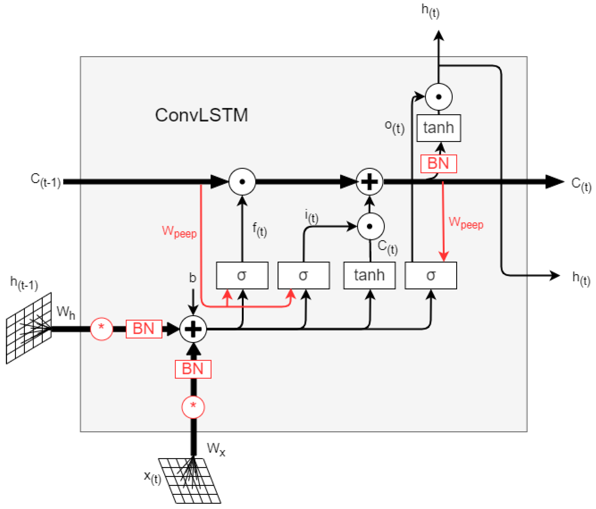
The long short-term memory (LSTM) network [18] increases the gating mechanism to control the information accumulation speed on the basis of the RNN network. However, LSTM is fully connected and spatial characteristics of the data cannot be analyzed. Therefore, SHI et al. [19] changed the fully connected operation to convolution on the basis of LSTM, then the ConvLSTM neural network was proposed. Figure 1 shows the ConvLSTM neural network structure, and its formula is as follows:
where stand for the convolution operation; represent the input gate, the forgetting gate, the output gate, the memory unit, and the external state, respectively; is a Logistic function; is the Hadamard operator; represents the weight of neurons.
Since the ConvLSTM network was composed of convolution operation and LSTM layers, the characteristics of both convolution and LSTM will affect the network performance. The operation of the convolution layer was usually regarded as the operation of aggregating spatial information and feature dimension information on the local receptive field, but it is quite difficult to learn big data by convolution operation alone. Therefore, many works have been proposed to improve network performance, such as the introduction of the attention mechanism, the introduction of the temporal convolutional network, and other methods, but these methods improved network performance from the spatial dimension. For convolution operations, if the features can be recalibrated, then there was no need to introduce spatial dimensions to improve network performance, which can reduce the difficulty of network training and can automatically obtain the importance of each feature, improve the important features, and reduce the features that are not useful for the current task. Therefore, the Squeeze-and-Excitation [20] (SE) module was proposed, as shown in Figure 2, and its formula is as follows:
where , and ; represents the convolution kernel of channels, represents the activation function RELU, and , .
The SE module was embedded in the ConvLSTM neural network to improve the channel attention ability of the network. The SE-ConvLSTM neural network is shown in Figure 3, and relevant parameters associated with each layer are shown in Table 1. The whole network structure consisted of a ConvLSTM layer, a Maxpooling layer, a Fully Connected layer, a Dropout layer, and an SE module.
In the proposed SE-ConvLSTM model, the first ConvLSTM layer adopted a large convolution kernel to extract more local features. In order to suppress over-fitting, the remaining ConvLSTM layers adopted small convolution kernels and added maxpooling layers to abstract futures, reducing network parameters and redundancy. At the end of the network, 3 fully connected layers were set, and the last layer was a single neuron as the output—HI. At the same time, in order to prevent overfitting and enhance the robustness of the network, the dropout layer was added to the fully connected layer.
2.2. Data Processing and Characteristic Index Construction
In the process of data collection, due to the factors of noise and other disturbances, it was difficult to ensure the purity of the original vibration data. In the area of signal processing, Variational Modal Decomposition (VMD), Empirical Mode Decomposition (EMD), and Ensemble Empirical Mode Decomposition (EEMD) algorithms had advantages and disadvantages in the field of signal processing. Compared with other algorithms, EEMD can decompose signals adaptively and effectively avoid modal aliasing [21]. In this paper, the EEMD algorithm was used to process the original signal before network training. The main steps of EEMD were as follows [22]:
- (1)
- Set the original signal processing times n.
- (2)
- Add Gaussian noise to n group of signals randomly to obtain a new signal.
- (3)
- The IMF components were obtained by EEMD decomposition of the new signal.
- (4)
- The mean value of IMF components of corresponding modes was calculated to obtain the decomposition result of EEMD.
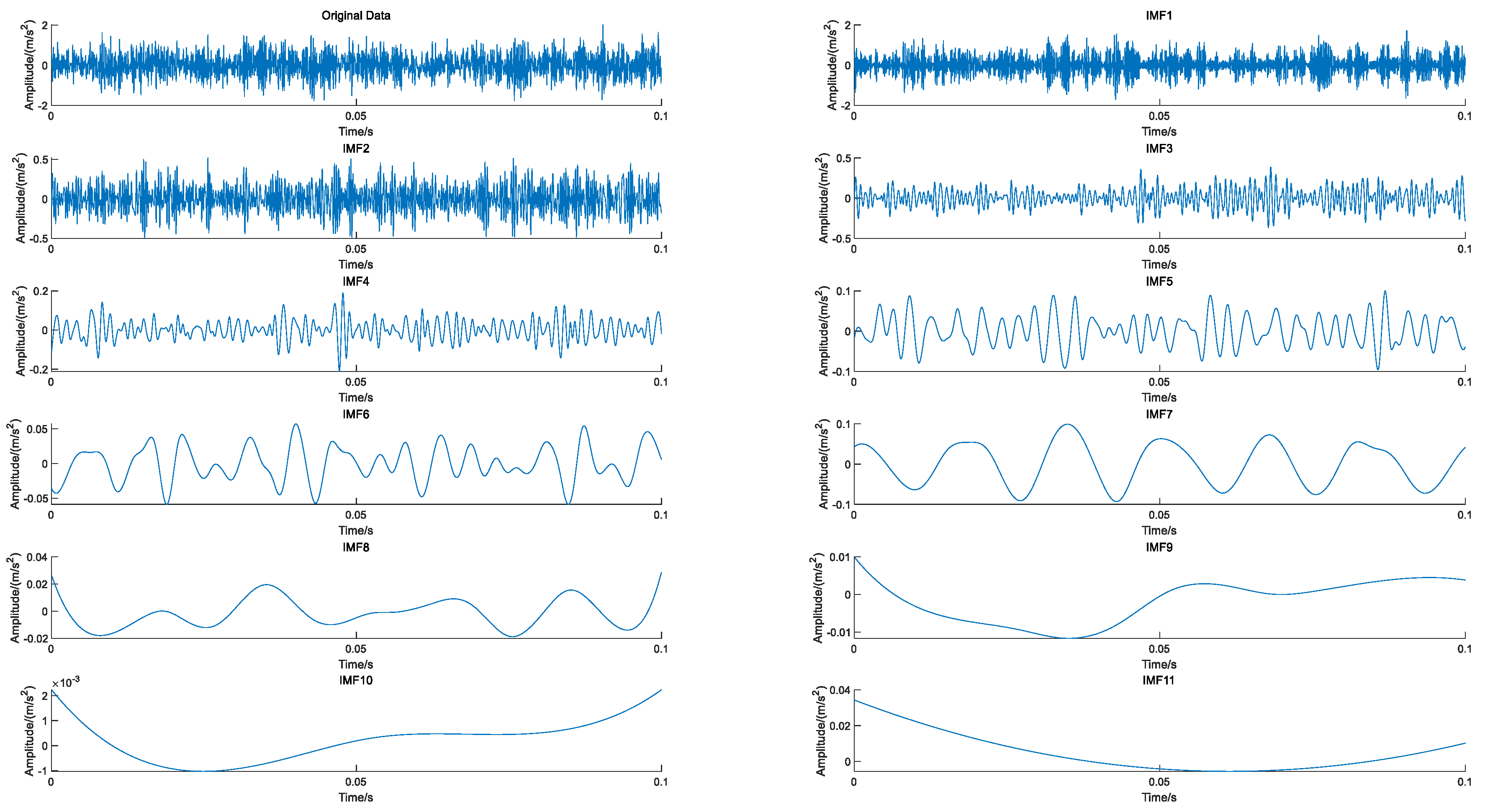
Since kurtosis can reflect the impact on the bearing during operation, after the EEMD generated 11 components, the components whose kurtosis was greater than the original signal were selected for reconstruction. The kurtosis formula was as follows:
where is the mean of and is the standard deviation of .
The bearing signal processed by EEMD is shown in Figure 4. It can be found that the vibration signal of the bearing can be effectively decomposed from the original signal after EEMD.
Considering the actual situation of bearing degradation, in this paper, we suggest that the bearing degradation should not be simply set as a (0-1) straight line, but rather should be designed as three stages. Therefore, after extracting 11 frequency domain indicators of the bearing, PCA was used to fuse the 11 frequency domain features [23]. The 11 frequency domain indicators are shown in Table 2. Among them, there are two defined frequency domain indicators, which are the fifth center frequency and the tenth root mean square frequency, and the remaining 9 indicators are commonly used in the frequency domain. The basic principle of PCA is to transform the original variables with a certain correlation into a set of unrelated data through linear transformation, and its main formula was as follows:
where and are the original variable and the converted variable, respectively, is the transformation matrix, is the original variable dimension, and is the dimension of the variable after transformation; in this paper, = 1.
The LOF (Local Outlier Factor) algorithm was used to divide the life interval of the indicator generated by PCA reduction. The LOF algorithm is an unsupervised classification algorithm used to judge the degree of abnormality by comparing the density near the sample object with the density in the neighborhood. Its main formula was as follows:
Through the above data processing operation, the original signal can be denoised and divided into three stages of life intervals.
3. Health Indicator Model Based on SE-ConvLSTM
The model was built based on the SE-ConvLSTM neural network, and the output was realized through network stacking and interaction. In the network training stage, the training data of the input was , where is the sampling data with M time steps and the data length is N. is the degree of degradation corresponding to the time t. In order to fully train and prevent the over-fitting phenomenon of the model, the sampling time step was set to 5, as shown in Figure 3. The network loss function was defined as:
where represents the true label and represents the model output.
After the HI output, this paper establishes a double exponential model to realize the bearing life prediction, and its formula is as follows:
where represents the health status of the bearing, and are the parameters of the double exponential model, which will be updated in the stage of particle filter prediction of remaining useful life.
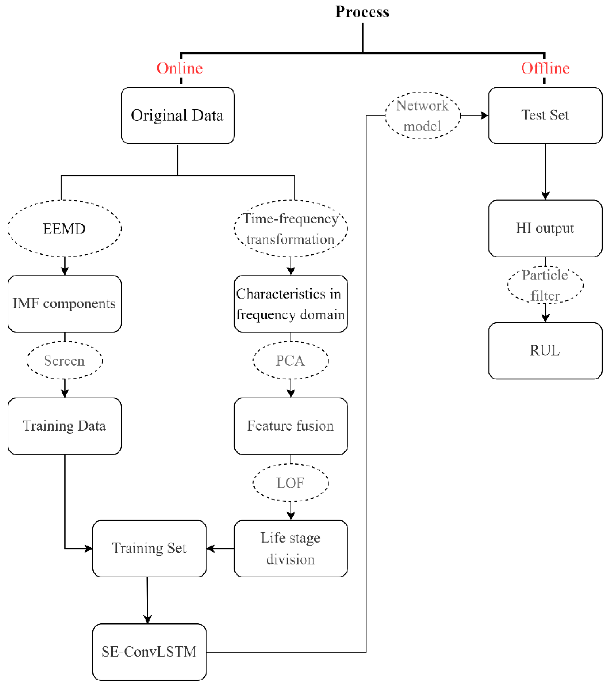
As the model established, HI can be output based on the SE-ConvLSTM neural network model, and then the double-exponential model can be updated by particle filtering to realize the RUL prediction. The specific process is shown in Figure 5.
4. Test Verification
In this paper, the public dataset IEEE PHM2012 Bearing accelerated aging data [24] was used to conduct experimental verification of the proposed model. The test data came from the PRONOSTIA test rig, which carried out accelerated life degradation tests on bearings and collected vibration signals within several hours, with a sampling frequency of 25.6 kHz; each sample was 0.1 s, and the samples were sampled every 10 s. This dataset contained 17 bearings in 3 working conditions. As shown in Table 3, the first two bearings of each working condition were used as training sets, and the other bearings were used as test sets. The test rig is shown in Figure 6.
The computer configuration used in the laboratory was as follows: The CPU was Intel(R) Core i7-8750H, the RAM was 16 GB, the GPU was Nvidia GeForce GTX 1060, and the programming language was Python 3.6.2 (64-bit), based on TensorFlow-GPU 2.4.0 deep Learning framework implementation.
Firstly, the bearing dataset was denoised and divided into degenerate intervals. The training data, Bearing1_1, were taken as an example, and its time domain signal is shown in Figure 7. This shows the whole life data, and at the end of life, with the aggravation of the damage, the vibration amplitude increased significantly, showing a trend of divergence.
According to the data processing process mentioned above, EEMD was firstly used for denoising the original data, and the 11 IMF components decomposed by EEMD are shown in Figure 8. Then, based on the kurtosis criterion described in Chapter 2, the components with kurtosis greater than the original signal were selected for reconstruction, as shown in Figure 9. The kurtosis values of IMF1, IMF2, and IMF3 were larger than the original signal, so these three components were selected for signal reconstruction, and then 11 frequency domain features were extracted, as shown in Figure 10. Subsequently, the PCA fusion algorithm was used for feature fusion. Then LOF algorithm was used to divide the degraded interval operation on the basis of the fused feature indicator. Finally, this paper designed a three-stage feature indicator. The data processing flow is shown in Figure 11.
The processed data were imported into the proposed SE-ConvLSTM model for training and compared with reference [25] and a classic CNN. In order to effectively evaluate the health indicators, after the network training, the monotonicity and trend analysis of HI were conducted [26], and the formula was as follows:
where , are the positive and negative values of the time derivative of HI. and represent the mean of and .
The monotonicity and trend results are shown in Table 4. It can be seen from Table 4 that the proposed model had better monotonicity and tendency.
In addition, in order to evaluate the data processing method and the SE-ConvLSTM neural network proposed in this paper, an ablation study was conducted, and the following three models were designed and compared:
- (1)
- Original data and SE-ConvLSTM neural network were used for training.
- (2)
- Processed data and ConvLSTM neural networks without the SE module were used for training.
- (3)
- Processed data and the SE-ConvLSTM neural network were used for training.
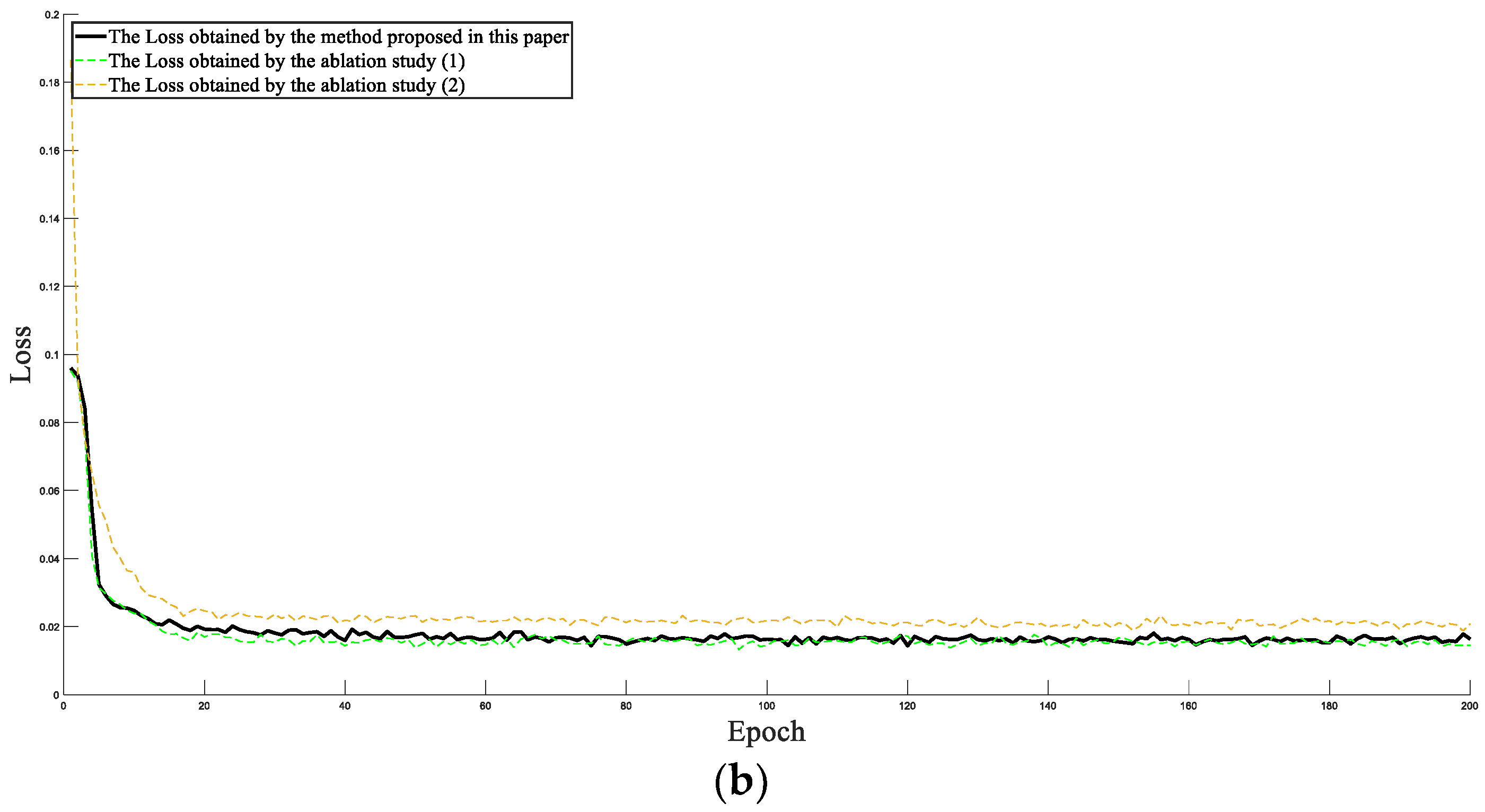
By comparing the HI output results and loss, the above three models were used to analyze the superiority of the proposed method. It can be seen from Figure 12 that the training process of the proposed method was relatively stable, and the failure threshold of the output HI was 1. However, it can be seen from Figure 12a that HI fluctuates greatly in the training process of (1) and (2), and the failure threshold of (1) was not stable to 1, but rather between 0.8 and 0.9, which will have a negative effect on the subsequent remaining useful life prediction. In addition, it can be seen from Figure 12b that the loss of the training process of the method proposed in this paper was stable between 0.01 and 0.02, indicating that the fitting effect of the label and data was relatively stable. By comparing the loss of (1) and (2), although the loss tends to be stable due to the network effect, combined with the output HI and loss values, the overall effect was not as good as the method proposed in this paper.
In order to analyze the hidden layer characteristics of the proposed model, the t-SNE algorithm [27] was used for visual analysis. The training data Bearing1_1 were taken as an example, where the selected hidden layers were the input layer, the first maxpooling layer, and the last fully connected layer, and the results are shown in Figure 13. Each point in Figure 13 represented the feature distribution at different times t. It can be seen from Figure 13 that, with the deepening of neural network layers, the training data changed from chaotic to ordered, which can reflect the bearing degradation process.
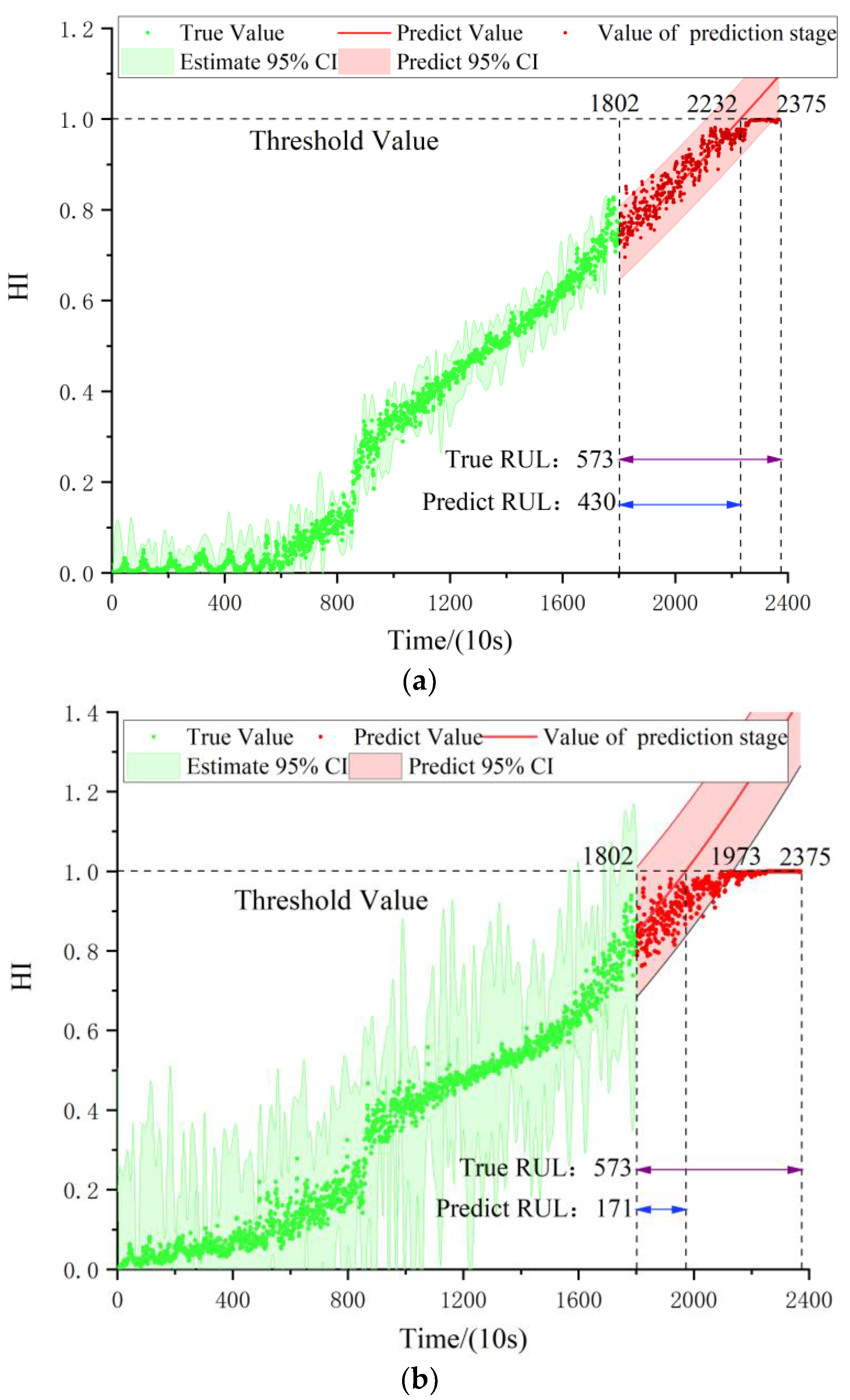
Then 11 test bearings were tested on the trained model. Taking Bearing1_3 as an example, the particle filter was used to predict the remaining useful life of the HI output from the model. The prediction results are shown in Figure 14, where the red curve is the HI predicted by the double exponential model. Figure 14a is the RUL result of the model proposed in this paper, and it can be seen that the threshold value of 1 is reached at period 2232, so the predicted remaining useful life is 430 (10 s). Figure 14b shows the predicted result of the LSTM neural network. It can be seen that the threshold value of 1 is reached at the time of cycle 1973, so the predicted remaining life is 171 (10 s). Figure 14c shows that for the prediction result of the classical convolutional neural network CNN, its threshold value of 1 is reached at period 2232, so the predicted RUL is 288 (10 s).
It can be seen from Figure 14 that when the red curve reached the threshold of 1, it represented the termination of remaining useful life. The prediction error (33.86%) and 95% Confidence Interval (CI) of the proposed method are higher than those of the other two methods (77.31% and 49.74%). The results of other test sets are shown in Table 5. The method proposed in this paper was also compared with other methods to reflect its superiority. For example, to achieve the prediction of RUL, Guo et al. [28] proposed a prediction model based on EMD-RISI-LSTM, as shown in reference [11]. Sensitive indicators and an RNN are used to predict the remaining useful life. In order to describe the superiority of this model, the absolute mean error was adopted to evaluate the model results, and its formula was as follows:
where represents the true life of group test data and represents the predicted life of group test data.
5. Conclusions
The accuracy of health indicator construction directly affected the precision of remaining useful life predictions of bearings. In this paper, a bearing health index construction model based on a three-stage life interval partition and SE-ConvLSTM was proposed, and the remaining useful life prediction method was obtained by combining it with a particle filter. After verification on the IEEE PHM2012 bearing dataset, the results showed that the method proposed in this paper has higher accuracy. The following conclusions were drawn from the experimental analysis:
- (1)
- Proposed the SE-ConvLSTM health index construction model, which realized the bearing health index output by utilizing the time and space characteristics of the convolutional long short-term memory neural network and attention mechanism of the SE Block.
- (2)
- Machine learning algorithms including EEMD and LOF were used to divide the bearing degradation interval, and then we constructed a health indicator in line with the bearing degradation process. By comparison, it was concluded that the three-stage performance indicator proposed in this paper predicted the bearing’s remaining useful life with higher accuracy and had important reference significance for bearing health evaluations.
6. Discussion
The degradation process of bearing performance in the whole life cycle is a complex nonlinear process. However, traditional neural-network-based methods usually consider the bearing performance degradation process to be linear, which does not conform to the actual situation of bearing degradation. Therefore, considering the actual situation of bearing degradation, this paper divides the bearing life cycle and designs a three-stage label. However, in actual engineering, due to practical problems such as changes in working conditions and frequent shutdowns, it is not easy to obtain full-life-cycle data of bearings. Therefore, data mining should be more in-depth, the division of the degradation stage should be clearer and more detailed, and it should be interpretable. Therefore, in future research, we should dive deeper into the process of bearing life evolution, learn from existing theories, start with practical problems, and conduct more in-depth research.
Author Contributions
S.Y. contributed to the theoretical algorithm, model training, and paper writing Y.L. (Yongqiang Liu). performed the algorithm improvement, paper revising, and language checking. Y.L. (Yingying Liao). helped perform the analysis with constructive discussions. K.S. contributed to the conception of the study. All authors have read and agreed to the published version of the manuscript.
Funding
The present work is supported by the National Key R&D Program (2020YFB2007700), the National Natural Science Foundation of China (Nos. 11790282; 12032017; 12002221 and 11872256), the S&T Program of Hebei (20310803D), the Natural Science Foundation of Hebei Province (No. A2020210028), and the Science Research Project of the Education Department of Hebei Province (Grant No. ZD2021093).
Institutional Review Board Statement
Not applicable.
Informed Consent Statement
Not applicable.
Data Availability Statement
The data that support this study are from the FEMTO-ST Institute (Besancon—France, http://www.femto-st.fr).
Conflicts of Interest
The authors declare no conflict of interest.
References
- Lei, Y.; Li, N.; Gontarz, S.; Lin, J.; Radkowski, S.; Dybala, J. A Model-Based Method for Remaining Useful Life Prediction of Machinery. IEEE Trans. Reliab. 2016, 65, 1314–1326. [Google Scholar] [CrossRef]
- Qiao, W.; Zhang, P.; Chow, M.Y. Condition Monitoring, Diagnosis, Prognosis, and Health Management for Wind Energy Conversion Systems. IEEE Trans. Ind. Electron. 2015, 62, 6533–6535. [Google Scholar] [CrossRef]
- Lei, Y.; Li, N.; Guo, L.; Li, N.; Yan, T.; Lin, J. Machinery health prognostics: A systematic review from data acquisition to RUL prediction. Mech. Syst. Signal. Process. 2018, 104, 799–834. [Google Scholar] [CrossRef]
- Wang, J.; Wen, G.; Yang, S.; Liu, Y. Remaining Useful Life Estimation in Prognostics Using Deep Bidirectional LSTM Neural Network. In Proceedings of the 2018 Prognostics and System Health Management Conference (PHM-Chongqing), Chongqing, China, 26–28 October 2018. [Google Scholar]
- Dong, S.; Wen, G.; Lei, Z.; Zhang, Z. Transfer learning for bearing performance degradation assessment based on deep hierarchical features. ISA Trans. 2020, 108, 343–355. [Google Scholar] [CrossRef]
- Zhang, J. Bearing Remaining Useful Life Prediction Based on a Scaled Health Indicator and a LSTM Model with Attention Mechanism. Machines 2021, 9, 238. [Google Scholar]
- Zhao, H.; Liu, H.; Jin, Y.; Dang, X.; Deng, W. Feature Extraction for Data-driven Remaining Useful Life Prediction of Rolling Bearings. IEEE Trans. Instrum. Meas. 2021, 99, 1. [Google Scholar] [CrossRef]
- Luo, J.; Zhang, X. Convolutional neural network based on attention mechanism and Bi-LSTM for bearing remaining life prediction. Appl. Intell. 2021, 52, 1076–1091. [Google Scholar] [CrossRef]
- Pavle, B.; Matej, G.; Dejan, P.; Juričić, D. Bearing fault prognostics using Rényi entropy based features and Gaussian process models. Mech. Syst. Signal. Process. 2015, 52–53, 327–337. [Google Scholar]
- Deng, F.; Bi, Y.; Liu, Y.; Yang, S. Deep-Learning-Based Remaining Useful Life Prediction Based on a Multi-Scale Dilated Convolution Network. Mathematics 2021, 9, 3035. [Google Scholar] [CrossRef]
- Guo, L.; Li, N.; Jia, F.; Jing, F. A recurrent neural network based health indicator for remaining useful life prediction of bearings. Neurocomputing 2017, 240, 98–109. [Google Scholar] [CrossRef]
- Zhang, A.; Wang, H.; Li, S.; Cui, Y.; Liu, Z.; Yang, G.; Hu, J. Transfer Learning with Deep Recurrent Neural Networks for Remaining Useful Life Estimation. Appl. Sci. 2018, 8, 2416. [Google Scholar] [CrossRef] [Green Version]
- Cao, Y.; Jia, M.; Ding, P.; Ding, Y. Transfer learning for remaining useful life prediction of multi-conditions bearings based on bidirectional-GRU network. Measurement 2021, 178, 109287. [Google Scholar] [CrossRef]
- Mao, W.; He, J.; Zuo, M.J. Predicting Remaining Useful Life of Rolling Bearings Based on Deep Feature Representation and Transfer Learning. IEEE Trans. Instrum. Meas. 2019, 99, 1. [Google Scholar] [CrossRef]
- Sun, C.; Ma, M.; Zhao, Z.; Tian, S.; Yan, R.; Chen, X. Deep transfer learning based on sparse autoencoder for remaining useful life prediction of tool in manufacturing. IEEE Trans. Ind. Inform. 2018, 15, 2416–2425. [Google Scholar] [CrossRef]
- Zhang, S.; Ye, F.; Wang, B.; Habetler, T. Few-shot bearing fault diagnosis based on model-agnostic meta-learning. IEEE Trans. Ind. Appl. 2021, 57, 4754–4764. [Google Scholar] [CrossRef]
- Li, C.; Li, S.; Zhang, A.; He, Q.; Liao, Z.; Hu, J. Meta-learning for few-shot bearing fault diagnosis under complex working conditions. Neurocomputing 2021, 439, 197–211. [Google Scholar] [CrossRef]
- Hochreiter, S.; Schmidhuber, J. Long Short-Term Memory. Neural Comput. 1997, 9, 1735–1780. [Google Scholar] [CrossRef] [PubMed]
- Shi, X.; Chen, Z.; Wang, H.; Yeung, D.-Y.; Wong, W.-K.; Woo, W.-C. Convolutional LSTM network: A machine learning approach for precipitation nowcasting. Adv. Neural Inf. Process. Syst. 2015, 28. [Google Scholar]
- Hu, J.; Shen, L.; Sun, G. Squeeze-and-Excitation Networks. IEEE Trans. Pattern Anal. Mach. Intell. 2020, 42, 2011–2023. [Google Scholar] [CrossRef] [Green Version]
- Wu, Z.; Huang, N.E. Ensemble empirical mode decomposition: A noise-assisted data analysis method. Adv. Adapt. Data Anal. 2019, 1, 1–41. [Google Scholar] [CrossRef]
- Chen, J.; Li, X. Application of ensemble empirical mode decomposition to noise reduction of fatigue signal. J. Vib. Meas. Diagn. 2011, 31, 15–19. [Google Scholar]
- Abdi, H.; Williams, L.J. Principal component analysis. Wiley Interdiscip. Rev. Comput. Stat. 2010, 2, 433–459. [Google Scholar] [CrossRef]
- Nectoux, P.; Gouriveau, R.; Medjaher, K.; Ramasso, E.; Chebel-Morello, B.; Zerhouni, N.; Varnier, C. PRONOSTIA: An experimental platform for bearings accelerated degradation tests. In Proceedings of the IEEE International Conference on Prognostics and Health Management, PHM’12, Denver, CO, USA, 18–21 June 2012. [Google Scholar]
- Tang, G.; Zhou, Y.; Wang, H.; Li, G. Prediction of bearing performance degradation with bottleneck feature based on LSTM network. In Proceedings of the 2018 IEEE International Instrumentation and Measurement Technology Conference (I2MTC), Houston, TX, USA, 14–17 May 2018. [Google Scholar]
- Zhang, B.; Zhang, L.; Xu, J. Degradation Feature Selection for Remaining Useful Life Prediction of Rolling Element Bearings. Qual. Reliab. Eng. Int. 2016, 32, 547–554. [Google Scholar] [CrossRef]
- Laurens, V.D.M.; Hinton, G. Visualizing Data using t-SNE. J. Mach. Learn. Res. 2008, 9, 2579–2605. [Google Scholar]
- Guo, R.; Wang, Y.; Zhang, H.; Zhang, G. Remaining useful life prediction for rolling bearings using EMD-RISI-LSTM. IEEE Trans. Instrum. Meas. 2021, 70, 1–12. [Google Scholar] [CrossRef]
Figure 1.
ConvLSTM neural network.

Figure 2.
SE model.

Figure 3.
Schematic diagram of SE-ConvLSTM neural network.

Figure 4.
EEMD-processed original signal.

Figure 5.
Flow chart of the proposed model.

Figure 6.
Aging platform PRONOSTIA.

Figure 7.
Time domain signal of Bearing1_1.

Figure 8.
Original signal and EEMD decomposition results.

Figure 9.
Envelope kurtosis values of each component and original signal.

Figure 10.
Eleven frequency domain features.

Figure 11.
Data processing process.

Figure 12.
Comparison of ablation study. (a) The HI of training bearing 1_1 under three test conditions, (b) the loss of training bearing 1_1 under three test conditions.
Figure 12.
Comparison of ablation study. (a) The HI of training bearing 1_1 under three test conditions, (b) the loss of training bearing 1_1 under three test conditions.


Figure 13.
Hidden layer features displayed by t-SNE. (a) Input layer, (b) the first maxpooling layer, (c) the first fully connected layer.
Figure 13.
Hidden layer features displayed by t-SNE. (a) Input layer, (b) the first maxpooling layer, (c) the first fully connected layer.

Figure 14.
RUL results of Bearing1_3. (a) Remaining useful life prediction results based on the model presented in this paper, (b) remaining useful life prediction results based on the LSTM model, (c) remaining useful life prediction results based on the CNN mode.
Figure 14.
RUL results of Bearing1_3. (a) Remaining useful life prediction results based on the model presented in this paper, (b) remaining useful life prediction results based on the LSTM model, (c) remaining useful life prediction results based on the CNN mode.


Table 1.
Parameter configuration of the proposed network.
| Layer | Parameters | |
|---|---|---|
| ConvLSTM_1 | Filters = 20, kernel size = (64, 1). | |
| ConvLSTM_2 | Filters = 20, kernel size = (3, 1) | |
| ConvLSTM_3 | Filters = 1, kernel size = (1, 1) | |
| Maxpooling_1 | Pool size = (8,1,1) | |
| Maxpooling_2 | Pool size = (2,1,1) | |
| Flatten | None | |
| Dense_1 | Units = 3 | |
| Dense_2 | Units = 1, activation = sigmoid | |
| Dropout | Rate = 0.5 | |
| SE module | Global Average Pooling | None |
| Dense | Units = 4 | |
| RELU | None | |
| Dense | Passed by RELU | |
| Sigmoid | None | |
Table 2.
The characteristic parameters in frequency domain.
| Equation | Equation | ||
|---|---|---|---|
| 1 | 7 | ||
| 2 | 8 | ||
| 3 | 9 | ||
| 4 | 10 | ||
| 5 | 11 | ||
| 6 |
Table 3.
IEEE PHM2012 dataset.
| Condition | Condition 1 | Condition 2 | Condition 3 |
|---|---|---|---|
| Training Data | Bearing1_1 | Bearing2_1 | Bearing3_1 |
| Bearing1_2 | Bearing2_2 | Bearing3_2 | |
| Test Data | Bearing1_3 | Bearing2_3 | Bearing3_3 |
| Bearing1_4 | Bearing2_4 | ||
| Bearing1_5 | Bearing2_5 | ||
| Bearing1_6 | Bearing2_6 | ||
| Bearing1_7 | Bearing2_7 |
Table 4.
The monotonicity and tendency of HI.
| Proposed Method | LSTM | CNN | |
|---|---|---|---|
| Mon | 0.976 | 0.887 | 0.892 |
| Corr | 0.981 | 0.973 | 0.962 |
Table 5.
Prediction results and comparison of RUL.
| Test Data | Current Time | True RUL | Prediction RUL | Proposed Method | Reference [28] | Reference [11] | LSTM | CNN |
|---|---|---|---|---|---|---|---|---|
| (10 s) | (10 s) | (10 s) | (%) | (%) | (%) | (%) | (%) | |
| Bearing1_3 | 1802 | 573 | 430 | 33.86 | 17.28 | 43.28 | 77.31 | 49.74 |
| Bearing1_4 | 1139 | 289 | 330 | −14.19 | 40.34 | 67.55 | 61.08 | 57.85 |
| Bearing1_5 | 2302 | 161 | 134 | 16.77 | −27.33 | −22.98 | −25.33 | −39.91 |
| Bearing1_6 | 2302 | 146 | 122 | 16.44 | −34.25 | 21.23 | 16.26 | 22.46 |
| Bearing1_7 | 1502 | 757 | 701 | 7.40 | 5.15 | 17.83 | 20.74 | 18.47 |
| Bearing2_3 | 1202 | 753 | 485 | 35.59 | −11.69 | 37.84 | 40.17 | 38.08 |
| Bearing2_4 | 612 | 139 | 162 | −16.55 | −31.65 | −19.42 | 38.47 | −30.26 |
| Bearing2_5 | 2002 | 309 | 90 | 70.87 | −9.06 | 54.37 | 49.27 | 55.25 |
| Bearing2_6 | 572 | 129 | 130 | −0.78 | −13.95 | −13.95 | 24.91 | −20.65 |
| Bearing2_7 | 172 | 58 | 70 | −20.69 | 50.00 | −55.17 | −40.12 | −69.47 |
| Bearing3_3 | 351 | 83 | 74 | 10.85 | None | 3.66 | 12.84 | 12.54 |
| Er | 21.37 | 22.10 | 32.48 | 36.98 | 37.70 |
Publisher’s Note: MDPI stays neutral with regard to jurisdictional claims in published maps and institutional affiliations. |
© 2022 by the authors. Licensee MDPI, Basel, Switzerland. This article is an open access article distributed under the terms and conditions of the Creative Commons Attribution (CC BY) license (https://creativecommons.org/licenses/by/4.0/).
Share and Cite
MDPI and ACS Style
Yang, S.; Liu, Y.; Liao, Y.; Su, K. A New Method of Bearing Remaining Useful Life Based on Life Evolution and SE-ConvLSTM Neural Network. Machines 2022, 10, 639. https://0-doi-org.brum.beds.ac.uk/10.3390/machines10080639
AMA Style
Yang S, Liu Y, Liao Y, Su K. A New Method of Bearing Remaining Useful Life Based on Life Evolution and SE-ConvLSTM Neural Network. Machines. 2022; 10(8):639. https://0-doi-org.brum.beds.ac.uk/10.3390/machines10080639
Chicago/Turabian StyleYang, Shuai, Yongqiang Liu, Yingying Liao, and Kang Su. 2022. "A New Method of Bearing Remaining Useful Life Based on Life Evolution and SE-ConvLSTM Neural Network" Machines 10, no. 8: 639. https://0-doi-org.brum.beds.ac.uk/10.3390/machines10080639
Note that from the first issue of 2016, this journal uses article numbers instead of page numbers. See further details here.