Article

Fault Diagnosis of Rolling Bearings Based on Variational Mode Decomposition and Genetic Algorithm-Optimized Wavelet Threshold Denoising

1
Hubei Provincial Industrial Safety Engineering Technology Research Center, Wuhan University of Science and Technology, Wuhan 430081, China
2
Key Laboratory of Metallurgical Equipment and Control Technology, Wuhan University of Science and Technology, Ministry of Education, Wuhan 430081, China
3
Hubei Key Laboratory of Mechanical Transmission and Manufacturing Engineering, Wuhan University of Science and Technology, Wuhan 430081, China
*
Author to whom correspondence should be addressed.
Submission received: 22 June 2022 / Revised: 20 July 2022 / Accepted: 1 August 2022 / Published: 4 August 2022

Abstract

:
Fault diagnosis of rolling bearings can be a serious challenge, as rolling bearings often work under complex conditions and their vibration signals are typically nonlinear and nonstationary. This paper proposes a novel approach to diagnosing faults of rolling bearings based on variational mode decomposition (VMD) and genetic algorithm-optimized wavelet threshold denoising. First, VMD was used to decompose the vibration signals of faulty rolling bearings into a series of band-limited intrinsic mode functions (BLIMFs). During the decomposition, the parameters of VMD were selected by Kullback–Leibler (K–L) divergence. Then, the effective BLIMFs were determined by the analysis of their correlation coefficients and variance contributions. Finally, genetic algorithm-optimized wavelet threshold denoising was proposed to optimize the selection of important parameters, and the optimized threshold function used not only ensures the continuity of the threshold function but also avoids the fixed deviation of the soft threshold. The validity and superiority of the proposed approach were verified by theoretical calculations, numerical simulations and application studies. The results indicate that the proposed approach is promising in fault diagnosis of rotary machinery.

1. Introduction

Bearings are common but essential machinery components. With high efficiency, low friction resistance, simple assembly, and easy lubrication, bearings are widely used in the machinery, electric power, mining, and aerospace industries [1]. Bearing damage affects the safety and normal operation of the equipment directly, and therefore bearing fault diagnosis is critically important. Bearing faults are usually caused by improper installation, overloading, poor lubrication, foreign body invasion, or other external factors [2]. In engineering practice, bearing monitoring is often accompanied by noise interference whose impact on bearing fault diagnosis is very significant, and so effective separation of fault signals from noise is a vital part of fault diagnosis.
The vibration signals of rolling bearings are typically nonlinear and non-stationary, and the commonly used noise reduction methods include fast Fourier transform (FFT), wavelet transform (WT), empirical mode decomposition (EMD), and empirical wavelet transform (EWT). FFT is a fast way to compute the discrete Fourier transform (DFT) of a sequence or its inverse [3]. FFT computes such transforms quickly by decomposing the DFT matrix into a product of sparse factors, so it can compute the complexity of the DFT, reducing the time required to define the computation when using the DFT. Zheng et al. [4] proposed a new spectral envelope-based adaptive empirical Fourier decomposition (SEAEFD) method to improve the performance of adaptive empirical Fourier decomposition (AEFD) for the analysis of vibration signals.
The noise reduction in vibration signals by WT falls into three categories: modular maximum noise reduction, threshold noise reduction, and spatial correlation noise reduction. Mallat et al. [5] proposed a modulus maximum noise reduction method, which judges the noise and denoise of the signals on the basis of the Lipschitz exponent. Donoho et al. [6,7] presented a threshold noise reduction method, which, based on the method of all threshold risks and the optimal estimation diagonal operator, obtains a threshold for dividing signals and wavelets, also called the universal threshold. The threshold function suggested by Yang et al. [8] is between hard and soft thresholding functions, but high frequency signals zeroed out, resulting in excessive noise reduction. Liu et al. [9] proposed a continuous function to remove gyroscopic noise, but it is non-differentiable at the threshold.
EMD decomposes nonlinear and non-stationary signals into a finite number of intrinsic mode functions (IMFs) [10,11], which resolves the problem of adaptive basis function unavailable. Xiong et al. [12] used EMD to denoise and remove trend terms from the vibration signals, and then employed the Alpha stable distribution to diagnose the faults of low-speed bearings. However, EMD has some inherent defects, for which scholars have proposed different improved algorithms, such as ensemble empirical mode decomposition (EEMD) [13,14], complete ensemble empirical mode decomposition (CEEMD) [15], complete ensemble empirical mode decomposition with adaptive noise (CEMDAN) [16,17] and so on. EWT is a non-stationary signal processing method proposed by Gilles [18]. It provides a new adaptive time-frequency analysis of signals by combining the adaptive decomposition concept of EMD and the compact support framework of wavelet transform theory.
Although EMD and its improvement are all adaptive, there exists the phenomenon of mode mixing. Dragomiretskiy et al. [19,20] proposed an adaptive decomposition, variational mode decomposition (VMD), to obtain the center frequency and bandwidth by iteratively searching for the optimal solution and then the mode function, which effectively suppresses mode mixing. VMD boasts a more solid mathematical foundation and can reduce the non-stationarity of time series with high complexity and strong nonlinearity, suitable for non-stationary sequences. In addition, it has the characteristics of Wiener filtering, which can remove noise more effectively. Xiang et al. [21] successfully applied the VMD algorithm to rotor fault diagnosis. Zhao et al. [22] proposed a method that combines VMD with singular value decomposition, and uses the noise reduction ability of singular value decomposition to further denoise the reconstructed signals after VMD to enhance fault information. While VMD also has its shortcoming, artificial selection of the decomposition mode number K and the penalty factor α will affect the decomposition effect. Therefore, this paper uses the K–L divergence method to optimize the parameters.
Since the vibration signals of rolling bearings are easily affected by strong background noise, signal acquisition and transmission equipment, use of VMD alone for fault feature extraction is undesirable in effect and further noise reduction is needed. The most commonly used WT denoising algorithm is the threshold noise reduction algorithm, which uses a soft or hard threshold function. However, the hard threshold function is discontinuous, resulting in local oscillation of the reconstructed signals, while the use of the soft threshold function introduces a constant deviation between the wavelet coefficients, leading to decreased accuracy of the reconstructed signals. Aimed at the deficiencies of soft and hard threshold functions, this paper proposed a genetic algorithm-optimized wavelet threshold denoising approach. The optimized threshold function used not only ensures the continuity of the threshold function but also avoids the fixed deviation of the soft threshold. This denoising approach achieved better noise reduction effect by adjusting three key parameters. To avoid the uncertainty of artificial selection of parameters, this paper used genetic algorithm to determine the optimal parameter value for better noise reduction.
Based on VMD and the proposed genetic algorithm-optimized wavelet threshold denoising approach, this paper presented a novel approach for the fault diagnosis of rolling bearings and verified the approach by means of simulations and actual measurement of bearing fault signals. The results were compared with those of EMD, CEEMD, EWT and CEEMDAN-wavelet packet threshold (CEEMDAN-WPT) combined denoising methods, pointing to the superiority of the proposed approach. It can effectively remove noise from bearing vibration signals, thus resolving equipment detection problems in engineering practice.

2. Methodologies

2.1. VMD

The VMD process solves a variational problem. In this algorithm, a BLIMF is defined as an amplitude modulation–frequency modulation function with bandwidth limitation, and the function of the VMD algorithm is to construct and solve the constrained variational problem [23]. Decomposing the original signals into a specified number of BLIIMF components can avoid mode mixing for an appropriate mode number K. The specific VMD process is shown in Figure 1.
This VMD also has shortcomings in that artificial selection of important VMD parameters, including the mode number K and penalty factor α , cannot yield the best results, rendering it necessary to simply and directly select the optimal parameters. In this paper, the K–L divergence, which is a description of the relationship between two probability distributions P and Q, was used to optimize the parameters [24]. K–L divergence can be defined as
D K L ( P Q ) = i p ( i ) log P ( i ) Q ( i )
P ( x ) = 1 n h i = 1 n k [ x i x h ]   ,   x R
k ( u ) = 1 2 π e u 2 / 2
where P(x) is the kernel density estimation; k(u) the kernel function; h a given positive number, usually called the window width or smoothing parameter.
In the real situation, the distribution of the signal is always unimodal and symmetrical, so Equation (1) becomes the K–L divergence in the symmetrical form, which can be defined as
D ( P , Q ) = D K L ( P Q ) + D K L ( P Q )
According to the given formulas, the divergence of D (P, Q) can be finally obtained. In practical applications, P represents the real distribution of the observed data, and Q the distribution of the theoretical data. By investigating the relationship between the theoretical sub-signal and the actual original signal, the best sub-signal was selected for analysis. The smaller the K–L divergence value, the closer the relationship is, and the theoretical sub-signal is the true component of the signal; otherwise, it is the false component.

2.2. Optimized WT Denoising

Common threshold functions include hard and soft threshold ones [25]. The hard threshold function is
w ^ j , k = { s g n ( w j , k )     w j , k | w j , k | λ 0 | w j , k | λ
and the soft threshold function is
w ^ j , k = { s g n ( w j , k )     ( | w j , k | λ ) | w j , k | λ 0 | w j , k | λ
Dai et al. [26] proposed a new threshold function based on the hard threshold one, called a semi-hard threshold:
W ^ j , k = { W j , k | w j , k | a 0 | w j , k | < b L a a b L ( W j , k b L ) other
This function divides the wavelet domain into three parts. When | W j , k | a ,   | W j , k | < b L , it is consistent with the hard threshold function, but when b L | W j , k | < a , it promises better continuity than the hard threshold function. The disadvantage is that the function is not continuous when | W j , k | a . This paper improved on this to overcome the shortcomings of the above scheme and proposed an optimized wavelet threshold denoising as
w ^ j , k = { s g n ( w j , k ) × ( | w j , k | α λ 1 + | w j , k λ | ) | w j , k | a 0 | w j , k | < b L s g n ( w j , k ) × a a b L ( | w j , k | b L ) other
Equation (5) is discontinuous in the wavelet domain, Equation (6) has a constant deviation in the wavelet coefficient, and Equation (7) is also discontinuous when | W j , k | a . Taking a = b L = λ , and considering different values of α : (i) when α 0 , Equation (8) is equivalent to the hard threshold denoising method; (ii) when α 1 , Equation (8) is similar to the soft threshold denoising method; (iii) when 0 < α < 1 , the function is continuous in the wavelet domain, overcoming the discontinuity of the hard threshold function and reducing the deviation of the soft threshold function. The optimized wavelet threshold denoising avoids the problems of local oscillation and reduced precision of the reconstructed signals caused by the shortcomings of the traditional threshold denoising method, and improves the noise reduction ability.

2.3. Genetic Algorithm

The optimal values were obtained by using MATLAB’s genetic algorithm toolbox to improve the parameter settings in the wavelet threshold denoising. The results were optimized by modeling, packaging, objective function building, and solution running. The output and input values were set according to the evaluation index calculation codes. Since the default optimal solution of the genetic algorithm is the minimum value of the objective function, this paper took the inverse of the signal-to-noise ratio (SNR) as the output value of the adaptive function, and the three variables were α , a, and b.
Before running the genetic algorithm, four operating parameters must be set: the population size M, the crossover probability Pr, the mutation probability Pm, and the maximum evolutionary algebra T. These parameters have a significant influence on the solution and must be selected carefully [27].
(1)
The size of the initial population M specifies the number of individuals contained in the population and generally ranges from 20 to 100. Inbreeding occurs if the group size is too small, resulting in diseased genes; conversely, if the group size is too large, the convergence of the problem is difficult to achieve, leading to wasted resources and reduced robustness.
(2)
Crossover operation is the main method for generating new individuals in a genetic algorithm, so the crossover probability Pr should generally take a larger value. However, if Pr is too large, the good patterns in the group will be destroyed, which adversely affects the evolutionary operation. If Pr is too small, the speed at which new individuals are generated is slower. The recommended value of Pr is 0.4 to 0.99.
(3)
The mutation probability Pm controls how often the mutation operation is used. If Pm is too small, the population diversity declines too quickly, leading to the rapid loss of effective genes which is not easy to repair. If Pm is too large, although the population diversity is guaranteed, the probability of high-order patterns destroyed also increases. Therefore, the range of Pm is generally 0.0001–0.1.
(4)
The maximum evolutionary algebra T represents the termination condition of the genetic algorithm. If the T is too small, the algorithm cannot easily converge, and the population is not mature; if T is too large, the algorithm is already proficient or the population is too precocious, in which case it is impossible to obtain a converged solution. Generally, the value of T is set to be 100–500.
The operating parameters of the genetic algorithm used in this paper are shown in Table 1.

3. The Proposed VMD and Genetic Algorithm-Optimized Wavelet Threshold Denoising Approach

In this section, an approach to fault diagnosis of rolling bearings based on VMD and genetic algorithm-optimized wavelet threshold denoising is proposed and discussed. The specific steps of the approach are as follows:
(1)
VMD of faulty rolling bearing signals: K–L divergence is used to obtain the optimal penalty factor and mode number. After the determination of important parameters, the signals are decomposed into multiple BLIMFs by VMD. Then, the correlation coefficient and variance contribution rate of each component are analyzed, the effective components are screened out and the signals are reconstructed.
(2)
Wavelet decomposition of the reconstructed signals: The db4 wavelet base is selected, the decomposition level j is determined to be 3 [28] (see Appendix A for parameter selection), and then 3-level decomposition of the reconstructed signals is carried out.
(3)
Threshold compression of wavelet decomposition coefficients: The optimal parameters are selected by using the genetic algorithm, and then the optimized wavelet threshold denoising is used to perform threshold compression on the low-frequency coefficients from the first to the third layers to remove the noise components.
(4)
Signal reconstruction: Signals are reconstructed on the processed low-frequency coefficients from the first to the third layers and the high-frequency coefficients in the third layer.

4. Numerical Simulation

4.1. Establishment of Simulation Signals

The fault model is used to simulate the shock signal generated when there is a local defect in the bearing inner ring [29]. Gaussian white noise with a noise variance of 0.2 is added, and the simulated signal expression is
{ x ( t ) = s ( t ) + n ( t ) = i A i h ( t i T ) + n ( t ) h ( t ) = e x p ( C t ) cos ( 2 π f n t ) A i = 1 + A 0 cos ( 2 π f n t )
where s(t) is the periodic impact component, and n(t) Gaussian white noise component. The amplitude A0 is 0.3, transpose frequency f r 30 Hz, attenuation coefficient C 700, and resonance frequency f n 4 kHz. The sampling frequency f s is 16 kHz, and the number of analysis points 4096. The shock signal and the waveform and spectrum after noise addition are shown in Figure 2.

4.2. Simulation Signal Denoising

4.2.1. IMF and BLIMF Selection

The correlation coefficient represents the similarity between two signals, and the correlation coefficient between each component and the original signal can be calculated to determine the effective components. The larger the correlation coefficient, the more similar the component is to the original signal. According to the statistical significance of the factor analysis method, the variance reflects the fluctuation characteristics of the rolling bearing fault signals, and the variance contribution rate is a critical indicator of the relative importance of the factor. The higher the variance contribution rate of the factor, the greater its influence on the original signal. The correlation coefficient and variance contribution rate of each order component were calculated as follows [30].
x g = 1 N j = 0 N x ( j ) h i ( j + τ )
m s e b ( i ) = 1 N i = 0 k h i ( j ) 2 [ 1 N j = 0 N h i ( j ) ] 2 i = 1 n ( 1 N j = 0 N h i ( j ) 2 [ 1 N j = 0 N h i ( j ) ] 2 )
where h i is the i IMF or BLIMF components obtained after decomposition, x g ( i ) the correlation coefficient between the ith order IMF or BLIMF component and the original signal, m s e b ( i ) is the variance contribution rate of the component, N the signal length, and τ the time interval.

4.2.2. Comparative Analysis

By means of K–L divergence calculations, the optimal penalty factor for VMD was found to be 100, and the optimal number of modes is 3. Five algorithms were used to decompose the simulated signals. From Figure 3, it can be seen that the correlation coefficients and variance contribution rates of the components vary with algorithms. The variance contribution rate graph shows that the maximum variance contribution rates are 0.7413 and 0.8697 for the EMD and CEEMD algorithms, respectively. These results indicate that the first IMF component greatly influences the original signal. The first IMF (IMF1) has significant sensitivity information, so this component is retained.
IMF1 obtained by CEEMDAN has a large correlation and variance contribution rate and therefore is the signal component. Part of IMF2 is a noise component, and other components with low correlation are noise components, too. Therefore, IMF2 is denoised with the wavelet packet threshold and reconstructed with IMF1. The correlation coefficient of IMF2 decomposed by EWT is 0.9297, close to 1. Although the correlation coefficient of IMF1 is also high, its variance contribution rate is relatively small, so only IMF2 is retained. In the VMD algorithm, only BLIMF2 is retained after comparing the correlation coefficients and variance contribution rates.
The root-mean-square error (RMSE), signal-to-noise ratio (SNR), and signal-to-noise ratio gain (GSNR) of the denoised signals and the original signals were used to judge noise reduction [31]. RMSE reflects the difference between the original and denoised signals, with a smaller RMSE corresponding to better denoising. SNR and GSNR are traditional methods for measuring the noise in a signal. The higher SNR and GSNR, the better the filtering effect. The specific formulas are as follows:
R M S E = 1 N k = 1 N [ f ( k ) y ( k ) ] 2
S N R = 10 log k = 1 N f 2 ( k ) k = 1 N [ f ( k ) y ( k ) ] 2
G S N R = S N R d n / S N R n
where: f(k) is the noise signal, y(k) the signal after noise reduction, N the signal length, S N R d n the signal-to-noise ratio after denoising, and S N R n the signal-to-noise ratio of the original signal.
The results are shown in Table 2. From the three objective noise reduction indicators, it can be seen that the noise reduction effect using CEEMD and EMD is poorer than using the other three methods. Comparison of the proposed approach with EWT and CEEMDAN–WPT indicates that the proposed approach is far superior, as measured by RMSE, SNR, and GSNR, and the original signal integrity is preserved to the greatest extent in noise removal.

5. Actual Bearing Signal Noise Reduction

The data for a rolling bearing with inner ring failure were used to further verify the proposed approach. The experimental dataset was collected from the test rig shown in Figure 4a, the layout of the sensors is shown in Figure 4a, and acceleration sensors collected signals at a sample frequency of 10240 Hz. The structure diagram of the test rig is shown in Figure 4b. The fault rolling bearing was located in the outer bearing bracket. The experimental bearing model is SKF 6308, and the specific data are shown in Table 3. The time domain waveform of the rolling bearing vibration signal is shown in Figure 5.
The vibration signals are decomposed by the CEEMDAN, EWT and VMD algorithms. According to the K–L divergence optimization, the optimal penalty factor for VMD is 150, the optimal number of modes is 4, and the convergence tolerance is set to be 10−5. The number of CEEMDAN layers is 8, the NR of the white noise group is 100, the standard deviation Nstd = 0.2, and MaxIter = 5000. The EWT number is consistent with that of VMD.
The decomposition results are shown in Figure 6a–c. To better illustrate the decomposition effect of EWT, the time scale of EWT was set to be 0.1. The boundaries of the spectrum division of the CEEMDAN, EWT and VMD algorithms are given in Figure 7a–c. Figure 7a shows the spectrum division diagram of the CEEMDAN method. It can be observed that the seventh and eighth boundaries are relatively close and cannot be distinguished from the spectrum. The spectrum division of the EWT method is shown in Figure 7b, and the second and third boundaries are concentrated in the middle, almost overlapping and indistinguishable from the spectrum. In Figure 7c, the optimized VMD was decomposed into four BLIMFs components, the frequency range of BLIMF4 is 0–658 Hz, and the fault frequency is mainly in this region, indicating that the optimized VMD has a good effect.
Each component’s correlation coefficient and variance contribution rate are shown in Figure 8. It can be seen from Figure 8 that CEEMDAN is mainly concentrated in IMF1, whose correlation is very high (up to 0.86) and whose variance contribution rate reaches an astonishing 0.80, and a small number of signal features exist in IMF2. The variance contribution rate of EWT is mainly concentrated in IMF1 and IMF4. Figure 6 shows obvious periodic shocks in BLIMF1 and BLIMF2 after VMD.
Another set of VMD algorithms without parameter optimization was added as a control group. The number of decomposition layers was the same as for CEEMDAN, and the three components with larger variance contribution rates were also selected. An envelope spectrum analysis was performed on these components, and the results are shown in Figure 9. In Figure 9a, IMF1 after the CEEMDAN algorithm can yield f B P F I and 2 f B P F I , but in IMF2 only f B P F I was observed. In IMF1 and IMF7 of the EWT in Figure 9b, 2 f B P F I cannot be seen, and IMF8 yields nothing. In Figure 9c, the characteristic and rotational frequencies of the inner ring fault can be clearly seen. In Figure 9d, only BLIMF3 can identify both f B P F I and 2 f B P F I at the same time and the rest can only identify f B P F I .
Comparison shows that the VMD algorithm after parameter optimization is better than other methods. BLIMF1 and BLIMF2 decomposed by VMD were reconstructed, and the optimized threshold denoising was used for further denoising (see Appendix B for the code of the improved threshold denoising). The genetic algorithm was used to find the optimal solution for the three parameters of optimized wavelet threshold denoising, and the threshold of wavelet coefficients was adaptively modified. The parameter settings are shown in Table 1, and the running process of the genetic algorithm is shown in Figure 10.
After parameter-optimized VMD decomposition, the envelope spectrum of the bearing signals was obtained by further denoising using the improved threshold algorithm, as shown in Figure 11. Except for the highest peak rotation frequency of 22.5 Hz, the frequency has an obvious peak at 107.5 Hz, which is consistent with the inner ring fault frequency obtained by calculations. Besides, it can also be found that there are speed frequency sidebands around f B P F I and 2 f B P F I , which indicates that the bearing has been seriously damaged and needs to be replaced immediately. Finally, the RMSE values and SNRs of the other four methods after denoising are summarized in Table 4. The results show that the approach proposed in this paper can denoise the signals more effectively and extract fault features in a better way.

6. Conclusions

Aimed at the problem that the weak fault characteristics of rolling bearings can be easily covered by noise, this paper proposed a novel approach for fault diagnosis of rolling bearings based on VMD and genetic algorithm-optimized wavelet threshold denoising. The approach was validated by simulation and experimental signals, and the following conclusions were reached:
(1)
Artificial selection of parameters cannot yield the best results for VMD, so K–L divergence can be used to optimize the selection of parameters K and α in VMD to reduce decomposition uncertainty.
(2)
The optimized wavelet threshold denoising approach proposed not only ensures the continuity of the threshold function but also avoids the fixed deviation of the soft threshold.
(3)
The verification results of simulation and measured signals show that the proposed approach can reduce noise interference and accurately extract fault features. Compared with the EMD, CEEMD, CEEMDAN–WPT, and EWT algorithms, the proposed approach boasts better noise reduction capability and hence higher application value.

Author Contributions

Conceptualization, R.Y. and C.H.; methodology, C.H.; software, C.H; validation, C.H. and S.P.; formal analysis, C.H.; investigation, C.H. and S.P.; resources, R.Y.; data curation, R.Y. and Y.L; writing—original draft preparation, C.H.; writing—review and editing, Y.L. and R.Y.; supervision, F.X.; All authors have read and agreed to the published version of the manuscript.

Funding

This research work was supported by National Natural Science Foundation of China under Grant No. 51875416, Natural Science Foundation Innovation Group Program of Hubei Province under Grant No. 2020CFA033, and China Postdoctoral Science Foundation under Grant No. 2020M682492, which are greatly appreciated.

Institutional Review Board Statement

Not applicable.

Informed Consent Statement

Not applicable.

Data Availability Statement

Research data are not shared.

Conflicts of Interest

The authors declare that they have no known competing financial interests or personal relationships that could have appeared to influence the work reported in this paper.

Appendix A. Selection of Decomposition Parameters

Reference 25 used vibration signals of three kinds of rolling bearings, namely, the one with the inner ring fault, the one with the rolling element fault, and the one with the normal bearing and BP neural network, to train the results of three-layer and four-layer wavelet packet decomposition. Compared with the three-layer wavelet packet decomposition, the four-layer decomposition has a much higher error rate, so the number of decomposition layers selected in this paper j = 3.
In the time domain, the wavelet transform is expressed as the convolution of the signals and the wavelet basis function. Therefore, in the process of wavelet transformation, if the waveform contained in the signals is similar to the shape of the selected wavelet basis function, the signal features of the part similar to the wavelet basis function waveform contained in the signals will be amplified, while other features of different shapes will be amplified. Part of the signals will be suppressed, so as to achieve the purpose of extracting signal fault features. The similarity between the wavelet basis function and the impulse signals can be expressed as
λ = i = 1 n a i h i 2 s i
where: λ is the similarity coefficient, which is the dimensionless coefficient; s i is the area contained in each wave peak after the wavelet basis function is taken as the absolute value; h i is the maximum value of each wave peak after the wavelet basis function is taken as the absolute value; and a i is the wavelet basis function. The weighting coefficient of each wave crest after taking the absolute value is found using a i = h i max ( h i ) ; n is the number of wave crests after taking the absolute value of the wavelet basis function.
The correlation properties of the commonly used wavelet bases and the similarity coefficient with the shock signals are summarized in Table A1, and the wavelet base function waveform is shown in Figure A1. According to the correlation properties of wavelet bases, the db4 with the largest λ is finally selected.
Table A1. Properties of wavelet basis functions.
Wavelet FunctionHarrDaubechiesSymletsMeyerMorletCoiflet
SymmetryYesFar fromNear fromYesYesNear from
OrthogonalYesYesYesYesNoYes
BiorthogonalYesYesYesYesNoYes
Compact supportYesYesYesNoNoYes
CWTPossiblePossiblePossiblePossiblePossiblePossible
λ 6.56327.49706.36266.60827.21486.3298
Figure A1. (a) haar; (b) db4; (c) sym4; (d) meyer; (e) coif4; (f) morlet.
Machines 10 00649 g0a1

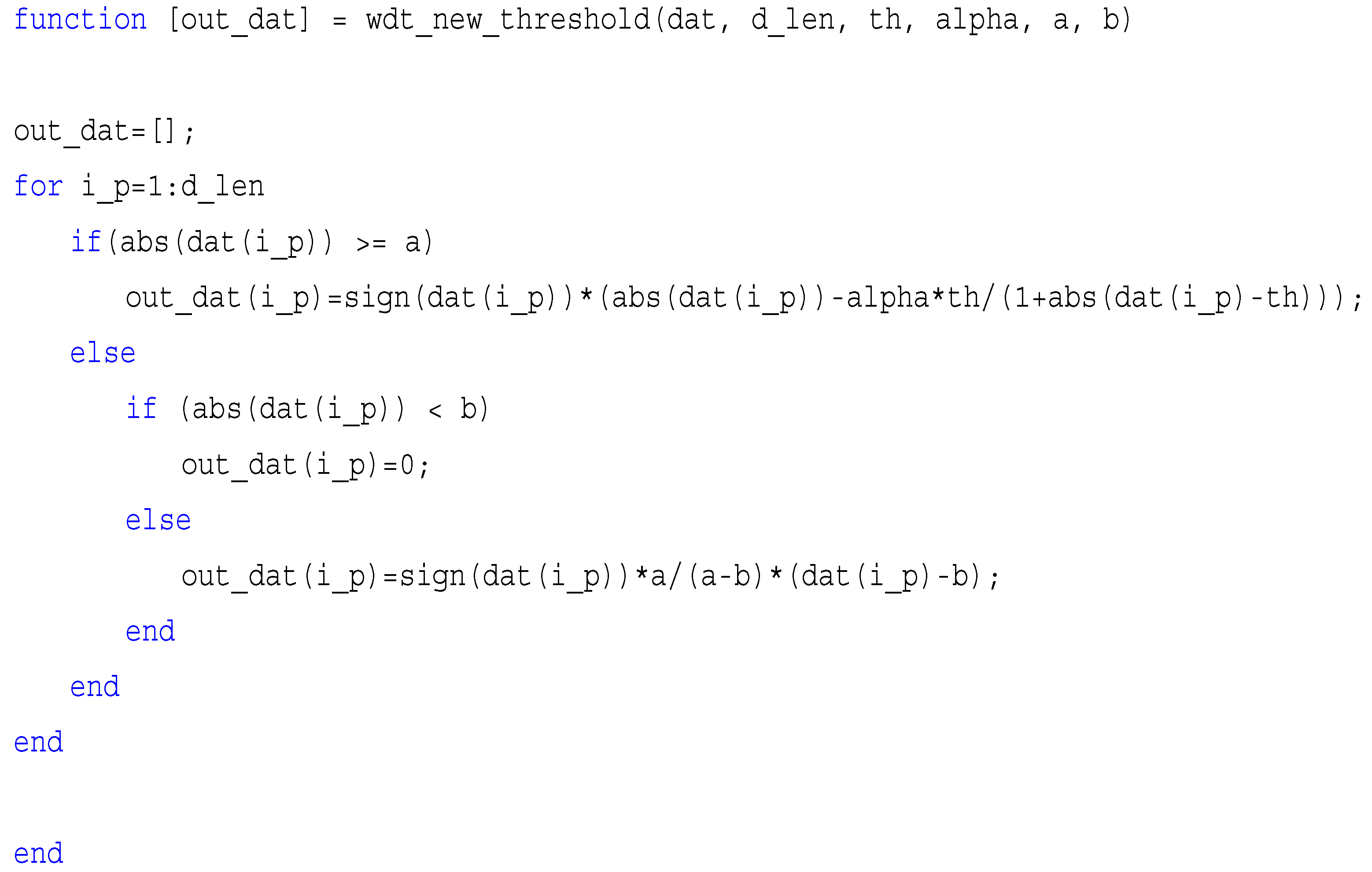
Appendix B. Code for Optimized Wavelet Threshold Denoising

Machines 10 00649 g0a2

References

  1. Lv, Y.; Yuan, R.; Song, G. Multivariate empirical mode decomposition and its application to fault diagnosis of rolling bearing. Mech. Syst. Signal Process. 2016, 81, 219–234. [Google Scholar] [CrossRef]
  2. Yuan, R.; Lv, Y.; Lu, Z.; Li, S.; Li, H. Robust fault diagnosis of rolling bearing via phase space reconstruction of intrinsic mode functions and neural network under various operating conditions. Struct. Health Monit. 2022, 14759217221091131. [Google Scholar] [CrossRef]
  3. Zheng, J.; Pan, H.; Cheng, J.; Bao, J.; Liu, Q.; Ding, K. Adaptive empirical fourier decomposition based mechanical fault diagnosis method. J. Mech. Eng. 2020, 56, 125–136. [Google Scholar]
  4. Sun, W.; An Yang, G.; Chen, Q.; Palazoglu, A.; Feng, K. Fault diagnosis of rolling bearing based on wavelet transform and envelope spectrum correlation. J. Vib. Control. 2013, 19, 924–941. [Google Scholar] [CrossRef]
  5. Chen, H.; Zheng, B. Signal noise reduction method of automata based on wavelet modulus maxima. Mech. Eng. Autom. 2010, 40, 36–37. [Google Scholar]
  6. Donoho, D.L.; Johnstone, I.M. Adapting to unknown smoothness via wavelet shrinkage. J. Am. Stat. Assoc. 1995, 90, 1200–1224. [Google Scholar] [CrossRef]
  7. Donoho, D.L.; Johnstone, J.M. Ideal spatial adaptation by wavelet shrinkage. Biometrika 1994, 81, 425–455. [Google Scholar] [CrossRef]
  8. Yang, H.; Wang, X.; Xie, P.; Leng, A.; Peng, Y. Wavelet infrared image denoising with improved correlation between threshold and scale. Chin. J. Autom. 2011, 37, 1167–1174. [Google Scholar]
  9. Liu, X.; Hu, J.; Gao, L.; Li, T.; Bai, X. Micromachined gyroscope denoising method based on improved wavelet threshold. Chin. J. Inert. Technol. 2014, 22, 233–236. [Google Scholar]
  10. Huang, N.E.; Shen, Z.; Long, S.R.; Wu, M.C.; Shih, H.H.; Zheng, Q.; Yen, N.-C.; Tung, C.C.; Liu, H.H. The empirical mode decomposition and the Hilbert spectrum for nonlinear and non-stationary time series analysis. Proc. R. Soc. Lond. Ser. A Math. Phys. Eng. Sci. 1998, 454, 903–995. [Google Scholar] [CrossRef]
  11. Alam, S.M.S.; Bhuiyan, M.I.H. Detection of seizure and epilepsy using higher order statistics in the EMD domain. IEEE J. Biomed. Health Inform. 2013, 17, 312–318. [Google Scholar] [CrossRef] [PubMed]
  12. Xiong, Q.; Xu, Y.; Peng, Y.; Zhang, W.; Li, Y.; Tang, L. Low-speed rolling bearing fault diagnosis based on EMD denoising and parameter estimate with alpha stable distribution. J. Mech. Sci. Technol. 2017, 31, 1587–1601. [Google Scholar] [CrossRef]
  13. Wu, Z.; Huang, N.E. Ensemble empirical mode decomposition: A noise-assisted data analysis method. Adv. Adapt. Data Anal. 2009, 1, 207152935. [Google Scholar] [CrossRef]
  14. Gaci, S. A new ensemble empirical mode decomposition (EEMD) denoising method for seismic signals. Energy Procedia 2016, 97, 84–91. [Google Scholar] [CrossRef] [Green Version]
  15. Yeh, J.R.; Shieh, J.S.; Huang, N.E. Complementary ensemble empirical mode decomposition: A novel noise enhanced data analysis method. Adv. Adapt. Data Anal. 2010, 2, 135–156. [Google Scholar] [CrossRef]
  16. Torres, M.E.; Colominas, M.A.; Schlotthauer, G.; Flandrin, P. A complete ensemble empirical mode decomposition with adaptive noise. In Proceedings of the 2011 International Conference on Acoustics, Speech and Signal Processing (ICASSP), Prague, Czech Republic, 22–27 May 2011; pp. 4144–4147. [Google Scholar]
  17. Lei, Y.; Liu, Z.; Ouazri, J.; Lin, J. A fault diagnosis method of rolling element bearings based on CEEMDAN. Proc. Inst. Mech. Eng. Part C J. Mech. Eng. Sci. 2017, 231, 1804–1815. [Google Scholar] [CrossRef]
  18. Gilles, J. Empirical wavelet transform. IEEE Trans. Signal Process. 2013, 61, 3999–4010. [Google Scholar] [CrossRef]
  19. Dragomiretskiy, K.; Zosso, D. Variational mode decomposition. IEEE Trans. Signal Process. 2013, 62, 531–544. [Google Scholar] [CrossRef]
  20. Zhang, X.; Chen, Y.; Jia, R.; Lu, X. Two-dimensional variational mode decomposition for seismic record denoising. J. Geophys. Eng. 2022, 19, 433–444. [Google Scholar] [CrossRef]
  21. Xiang, L.; Zhang, L. Application of variational mode decomposition in fault diagnosis of rotors. J. Vib. Test. Diagn. 2017, 37, 793–799. [Google Scholar]
  22. Zhao, H.; Guo, S.; Gao, D. Fault feature extraction of bearing faults based on singular value decomposition and variational modal decomposition. J. Vib. Shock. 2016, 35, 183–188. [Google Scholar]
  23. He, Y.; Wang, H.; Gu, S. A new method for bearing fault diagnosis based on VMD parameter optimization based on genetic algorithm. J. Vib. Shock. 2021, 40, 184–189. [Google Scholar]
  24. Xu, T.; Wang, H.; Song, Z.; Li, Y. Fault diagnosis of VMD instantaneous energy and PNN based on K-L dispersion. J. Electron. Meas. Instrum. 2019, 33, 117–123. [Google Scholar]
  25. Deng, P.; Zhang, L.; Liu, R.; Wang, B. Denoising of microgrid detection signal based on improved threshold function wavelets. Electr. Meas. Instrum. 2021, 58, 180–185. [Google Scholar]
  26. Dai, C.; Zhu, Y.; Chen, W. A New Wavelet Noise Cancellation Threshold Selection Method. Comb. Mach. Tool Autom. Mach. Technol. 2005, 6, 33–35. [Google Scholar]
  27. Wang, X.P.; Cao, L.M. Genetic Algorithm: Theory, Application and Software Implementation; Xi’an Jiaotong University Press: Xi’an, China, 2002; pp. 68–69. [Google Scholar]
  28. Jia, T. Research on the Fault Diagnosis of Rolling Bearings in the Running Section of Rail Trains; Beijing Jiaotong University: Beijing, China, 2011. [Google Scholar] [CrossRef]
  29. Tang, G.; Wang, X. Early fault diagnosis of rolling bearings fused with singular value differential spectra of IVMD. Vib. Test Diagn. 2016, 36, 700–707. [Google Scholar]
  30. Zheng, J.; Cao, S.; Pan, H.; Ni, Q. Spectral envelope-based adaptive empirical Fourier decomposition method and its application to rolling bearing fault diagnosis. ISA Trans. 2022. [Google Scholar] [CrossRef]
  31. Wang, H.; Bai, H.; Zhao, Y.; Wang, B.; Wang, H. Denoising Method of Blasting Signal Based on Fourier Decomposition-Wavelet Packet Analysis. Blasting 2021, 38, 37–44. [Google Scholar]
Figure 1. Illustration of the VMD algorithm.
Machines 10 00649 g001
Figure 2. Simulated signals: (a) pure signal waveform and spectrogram (b) simulated signal waveform and spectrogram.
Machines 10 00649 g002
Figure 3. Component correlation coefficient and variance contribution rate under the decomposition of five algorithms of rolling bearing: (a) EMD, (b) CEEMD, (c) VMD, (d) EWT, and (e) CEEMDAN.
Machines 10 00649 g003aMachines 10 00649 g003b
Figure 4. (a) The experimental rig and the location of the acceleration sensors. (b) The structure of test rig: 1—magnetic powder brake, 2—acceleration sensor, 3—helical gearbox, 4—shaft coupling, 5—planetary gearbox, 6—bearing bracket, 7—motor, and 8—outer bearing bracket.
Machines 10 00649 g004
Figure 5. Acceleration signal time domain waveform of inner race failure bearing.
Machines 10 00649 g005
Figure 6. Decomposition results of the three algorithms: (a) CEEMDAN, (b) EWT, and (c) VMD.
Machines 10 00649 g006aMachines 10 00649 g006b
Figure 7. The spectrum segmentation boundaries: (a) The boundary of CEEMDAN; (b) The boundary of EWT; (c) The boundary of VMD. The X and Y labels of all plots are “Frequency(/Hz)” and “Amplitude (/V)”, respectively. The same caption rule applies to all frequency domain plots hereinafter.
Machines 10 00649 g007aMachines 10 00649 g007b
Figure 8. Correlation coefficients and variance contribution rates of IMF components with three different algorithms.
Machines 10 00649 g008
Figure 9. Envelope spectrum: (a) CEEMDAN, (b) EWT, (c) VMD, and (d) VMD with unoptimized parameters.
Machines 10 00649 g009aMachines 10 00649 g009b
Figure 10. Genetic algorithm operation results.
Machines 10 00649 g010
Figure 11. The envelope spectrum of the signal after denoising.
Machines 10 00649 g011
Table 1. Operating parameters of genetic algorithm.
Genetic Algorithm ParametersValues
M50
Pr0.8
Pm0.01
T300
Table 2. Comparison of noise reduction effect of simulated bearing.
Noise Reduction MethodRMSESNRGSNR
EMD0.17403.42341.0583
CEEMD0.17973.47971.0814
EWT0.16873.94851.2271
CEEMDAN + WPT0.16973.66511.1499
The proposed approach0.09906.73502.1397
Table 3. Bearing parameters.
Bearing TypeSampling Frequency (Hz)Rotating Speed
(r/min)
Fault Characteristic Frequency (Hz)
SKF630810,2041309107.25
Table 4. Comparison of noise reduction effect of actual bearing.
Noise Reduction MethodRMSESNR
EMD0.35674.5971
CEEMD0.34654.6352
CEEMDAN-WPT0.32904.7264
EWT0.29955.5910
The proposed approach0.19817.1065
Publisher’s Note: MDPI stays neutral with regard to jurisdictional claims in published maps and institutional affiliations.

