A Hybrid Approach for Predicting Critical Machining Conditions in Titanium Alloy Slot Milling Using Feature Selection and Binary Whale Optimization Algorithm

Abstract

Monitoring the machining process is crucial for providing cost-effective, high-quality production and preventing unwanted accidents. This study aims to predict critical machining conditions related to surface roughness and tool breakage in titanium alloy slot milling. The Siemens SINUMERIK EDGE (SE) Box system collects signals from the spindle and axes of a CNC machine tool. In this study, features were extracted from signals in time, frequency, and time–frequency domains. The t-test and the binary whale optimization algorithm (BWOA) were applied to choose the best features and train the support vector machine (SVM) model with validation and training data. The SVM hyperparameters were optimized simultaneously with feature selection, and the model was tested with test data. The proposed model accurately predicted critical machining conditions for unbalanced datasets. The classification model indicates an average recall, precision, and accuracy of 80%, 86%, and 95%, respectively, when predicting workpiece quality and tool breakage.

1. Introduction

The fourth industrial revolution, known as Industry 4.0, has revolutionized manufacturing by reducing the need for human intervention. This revolution has led to lower prices and increased production volume. Industry 4.0 achieves this through automation and robotics, which lower labor costs and boost production. Additionally, the flexibility and customization capabilities of Industry 4.0 enable cost-efficient production of smaller batches and custom products, potentially resulting in decreased prices for machined and milled items [1]. The fourth generation industrial revolution was proposed by Kagerman et al. [2] due to the existing infrastructures of the world, such as universal access to the Internet and computer equipment, the reduction in the cost of providing computer parts, the expansion of IoT technology, and the growth of artificial intelligence.

As the global market grows, it is essential to have access to health monitoring and diagnosis tools, such as Tool Condition Monitoring (TCM) [3]. The TCM systems are used for real-time monitoring and predictions of when tools need to be changed during cutting processes. These systems are becoming increasingly important with the rise of flexible, intelligent, and computer-integrated manufacturing systems [4]. Various sectors in the industry have adopted hard-to-machine materials like Ti6Al4V for their strength, corrosion resistance, and extended creep life. However, their machinability is poor due to high cutting forces, high-temperature development, and severe work hardening. In this regard, correct prediction is crucial for optimizing machining efficiency, tool life, surface quality, and process stability, leading to competitive advantages and sustainable practices in industrial applications. TCM systems are needed to optimize tool life and boost production [5]. Tool monitoring detects tool problems before total failure, eliminating extra machining expenses by repairing or replacing the tool at the right moment [6]. Recently, artificial intelligence-based online tool monitoring has made significant progress. Intelligent models analyze data from various machining processes to classify different machining conditions as needed. There are two methods for monitoring machining processes: direct and indirect methods. Direct methods for monitoring machining processes involve measuring parameters using lasers, cameras, and ultrasonic devices. These methods are generally reliable but can become challenging in situations such as with a high-pressure coolant–lubricant. Most researchers have focused on indirect monitoring approaches to understand better the relationship between cutting tool conditions and variables such as cutting forces, vibration, and surface finish [6,7,8]. Feature-based monitoring techniques use features derived from sensor signals to detect the process condition [9]. It can achieve indirect monitoring by monitoring power signals, vibration, force, current consumption, audio emissions, and other relevant sensors. An indirect monitoring system involves signal registration, preprocessing, feature extraction (mainly in three domains: time, frequency, and time–frequency), feature selection, pattern recognition, and decision making [10]. Data analysis over time often involves statistical analysis, singular spectrum analysis (SSA), empirical mode decomposition (EMD), and principal component analysis. On the other hand, analyzing data in terms of frequency requires a fast Fourier transform (FFT) or power spectrum density (PSD). In TCM, the wavelet transform (WT), short-time Fourier transform (STFT), empirical wavelet transform (EWT), intrinsic time-scale decomposition (ITD), and Hilbert–Huang transform (HHT) are frequently used to examine signals simultaneously in both time and frequency domains [11,12,13,14]. Intelligentization of machining is a growing trend in the machining industry. Li et al. [15] developed a real-time tool breakage detection system that employs an acoustic emission (AE) sensor and an electric feed current sensor, utilizing a current sensor as an economic monitoring tool. The discrete wavelet transform (DWT) was used to analyze AE and feed electric current signals. The experimental results showed that the system could accurately detect tool breakage. Li et al. [16] studied tool breakage detection in end milling using the spindle current. A convolutional neural network (CNN) was adopted to detect tool breakage by analyzing the signal of the spindle current; CNN achieved a high accuracy rate (93%). The time domain analysis revealed that the spindle current could serve as an indicator of tool wear. This discovery implies that utilizing current to predict tool breakage is a feasible choice with promise for enhancement. Kolan et al. [17] present a system for monitoring drill tool wear through machine data. They investigate the correlation between directly measured flank wear ratio and indirect indicators like drive currents and workpiece vibration, showcasing significant correlations with wear via RMS signals. Tahir et al. [18] used three piezoelectric sensors to detect tool wear using cutting force signals in the time and frequency domain. Results showed that signal amplitudes of the main cutting force increase in the time domain as flank wear increases. In contrast, the amplitude peak in the frequency domain decreases with increased flank wear and cutting speed. Sensor fusion is an effective method to enhance monitoring systems by merging data from several sensors in a complementary manner. By adopting sensor fusion, more reliable data can be produced by adjusting the monitoring systems [19]. However, having excessive sensors can lead to an abundance of redundant and useless features, causing the monitoring system to become less effective and resilient [14]. Segreto et al. [11] developed a tool wear estimation method for Inconel 718 based on detecting cutting force, AE, and vibration acceleration signals. Wavelet packet transform (WPT) decomposition was employed to extract various signal features (SFs). The authors then utilized them to form multiple feature pattern vectors (FPVs) for artificial neural networks (ANNs). Results showed that the proposed method could accurately estimate cutting tool wear. Similarly, Niaki et al. [20] investigated the use of the recurrent neural network (RNN) with statistical features of WPD for TCM of hard-to-cut materials. In their study, sensory information from spindle power and vibration was utilized. The improved performance accurately estimated tool wear, increased productivity and quality, and reduced costs. He et al. [4] introduced a new way to predict tool wear during turning operations using temperature signals and a stacked sparse autoencoder (SSAE) model. Their method was more accurate and stable than traditional methods, and time–domain features of the temperature signal were highly related to tool wear. The authors suggest that incorporating temperature signals can be a reliable way to enhance wear predictions. Hojati et al. [21] proposed a model to predict critical machining conditions concerning surface roughness and tool breakage during the milling of a titanium alloy (Ti6Al4V). After collecting the process signals through a Siemens SINUMERIK Edge Box computing device, the Gramian angular field (GAF) and a CNN method were applied. The current investigation showed that the model achieved acceptable performance with recall and precision values of 75% and 88%, respectively, and the accuracy stood over 95% in different groups. The authors recommend that future improvements to the model should involve expanding the dataset, specifically by collecting more experimental data related to the critical machining condition. Aghazadeh et al. [19] present a methodology for tool wear monitoring using WT, spectral subtraction, and CNNs. The WT reveals the time-variant characteristics of the signal frequency response. At the same time, spectral subtraction removes the steady-state part of the signal due to regular cutting and magnifies the remaining fault characteristics. The CNNs accurately characterize internal variations within a large amount of data. Results show that the proposed methodology has an average accuracy of 87.2% and 81.5% with and without spectral subtraction, respectively. Pagani et al. [22] present a deep learning approach for tool wear assessment in machining operations. The method uses the monitoring feature of chip color characteristics like RGB and HSV image channels. It can process complex color distributions on the chips and classify the tool wear state. The method was tested on five different tools with five distinct cutting conditions. It could accurately predict tool wear with up to 97% accuracy. However, it was only suitable for fixed machining processes due to the influence of workpiece materials and cutting process parameters. The curse of dimensionality caused by large datasets with many features reduces machine learning model performance. It increases complexity and computational costs [23]. Dimensionality reduction techniques, such as feature selection and extraction, are used to address this issue. Feature selection removes redundant and irrelevant features to select the most optimal subset, while feature extraction generates smaller-dimensional features. Both approaches aim to improve model performance, prevent overfitting, and enhance speed [24]. Feature selection techniques are classified into filter, wrapper, and hybrid methods, each with advantages and limitations. Filter methods assign weights to features but ignore their relationships, while wrappers optimize feature sets at a higher computational cost. Hybrid approaches combine the benefits of both methods [12,23,24]. Maciej Kusy et al. [25] propose a feature selection approach for a milling process dataset, combining Pearson’s linear correlation coefficient, ReliefF, and the single decision tree methods. The approach identifies the most significant features and creates a reduced dataset, evaluated using computational intelligence models for classification tasks. The results confirm the effectiveness of the approach and suggest its universality for different classification problems. Further research will explore weighting the selected features based on classification correctness. Xie et al. [26] discuss using continuous hidden Markov models (CHMMs) for TCM and life prediction in CNC high-speed milling operations. The authors use Fisher’s discriminant ratio (FDR) as the criterion for feature selection. Ten top-value features are selected to establish the CHMMs. The proposed method uses two feature sets to monitor different tool wear conditions (medium and severe worn states). The results show that FDR is a robust feature-selecting algorithm that can distinguish severely worn tool states but has a poor ability to classify other states. Liao et al. [27] introduced a recognition scheme for tool wear states that relies on signal analysis and machine learning. The authors implemented feature extraction through time domain analysis, frequency domain analysis, and WPD. The feature selection module uses a genetic algorithm (GA) to select a subset of features that best predict tool wear. The tool wear state classification module that uses an SVM model optimized by the Grey Wolf Optimizer (GWO) algorithm. Chen et al. [28] studied chatter detection in a multi-channel monitoring system. The ensemble empirical mode decomposition (EEMD) decomposes the raw signals into intrinsic mode functions (IMFs) with various frequency bands. Features extracted from IMFs are ranked using the Fisher discriminant ratio (FDR) and presented to a linear SVM for classification. The most effective channel to detect chatter was identified in their work. The results showed that the multi-channel strategy achieved higher accuracy than the single-channel strategy. In a study conducted by Binsaeid et al. [29], they investigated the effectiveness of machine learning and machine ensemble techniques (such as majority vote and generalized stacking ensembles) for analyzing sensor signals (force, vibration, AE, and spindle power) in machining 4340 steel. They utilized a data acquisition and signal processing module to extract 135 features from the signals. By applying a correlation-based feature selection technique, they identified the most significant features. Surprisingly, they found that using a subset of 25 features outperformed all 138 features, which led to improved computational performance and greater efficiency in TCM modeling. Kossakowska et al. [30] presented a filter methodology for prominent SFs in tool wear diagnostics in the time, frequency, and time–frequency domains. The study did not find strong correlations with tool wear but proposed a large set of SFs that may be related to tool wear. The research findings suggest that no single SF is always associated with tool wear. For each new machining case, many different SFs should be determined, and those related to the tool state should be automatically selected. Hu et al. [14] investigated the tool wear mechanism in milling Ti–6Al–4V under minimum quantity lubrication (MQL) conditions. Cutting forces and AEs were measured online and used as raw sensor signals. The SFs were analyzed and extracted from the time and frequency domains. High-correlated features were selected based on mutual information (MI). Linear discriminant analysis (LDA) was used to reduce dimensionality. Then, the $v$-SVM was used to predict tool wear states. An overall classification rate of 98.9% was obtained. Liu et al. [9] evaluated the relationship between sound signals and tool wear under multiple cutting conditions. The WPD was used to extract time–frequency features from sound signals. This procedure was followed by a stepwise regression and an artificial neural network model to predict the degree of tool wear. The time–frequency feature extracted from the resonant bandwidth of the sound signal proved to have an apparent correlation with the flank wear of a CNC engraving machine and was invulnerable to background noise and robust under varying spindle speeds and feed rates. Lei et al. [31] proposed a tool wear estimation method based on an extreme learning machine (ELM) algorithm enhanced by a hybrid genetic algorithm and particle swarm optimization (GAPSO) (combination of GA and particle swarm optimization (PSO)) approach. Features extracted in the time, frequency, and time–frequency domains of the workpiece vibration signals were used as inputs for the ELM model. The hyperparameters of the ELM model are optimized based on the GAPSO approach with the training dataset. The results showed that the proposed method provided a considerably lower mean squared error (MSE) value and computation time than the ELM, GA-ELM, and PSO-ELM methods. This research was conducted in similar steps as conducted by Chegini et al. [12]. They presented a novel fault detection method for rotary machines using a wrapper and filter. The EMD and WPD were used to decompose and process vibration signals. Then, time–frequency domain features were utilized to construct the feature matrix. The proposed method combines both the F-score and Fisher discriminant analysis (FDAF-score) with the binary particle swarm optimization (BPSO) algorithm as feature selection technique. The goal is to determine the optimal feature set and optimize the SVM parameters. The proposed method can select features sensitive to the presence of defects in bearings, identify different fault sizes for the three faulty states in bearings, and solve the dimensionality problem of the feature space.

According to the literature, there is not only a gap in studying feature selection in machining processes, but this gap is also apparent in the simultaneous selection of the most appropriate features and optimization of a machine learning model. This study proposed a new method to predict critical machining conditions in titanium alloy slot milling, incorporating the Siemens SINUMERIK EDGE Box system as a sensor monitoring tool. The experiments were conducted on titanium alloy (Ti6Al4V), known for causing severe tool wear, breakage, and increased surface roughness. Extracting statistical features from the signals collected in three domains was performed to achieve accurate predictions of critical machining conditions. A feature selection method was employed, combining a t-test filter technique criterion with a BWOA.

Additionally, the study optimized the hyperparameters of the SVM model using a whale optimization algorithm, ensuring optimal performance. In order to address the challenge of dimensionality, the study employed dimensionality reduction techniques, including feature selection and extraction methods. In addition, a novel K-fold cross-validation division method was introduced to split the data into twenty groups.

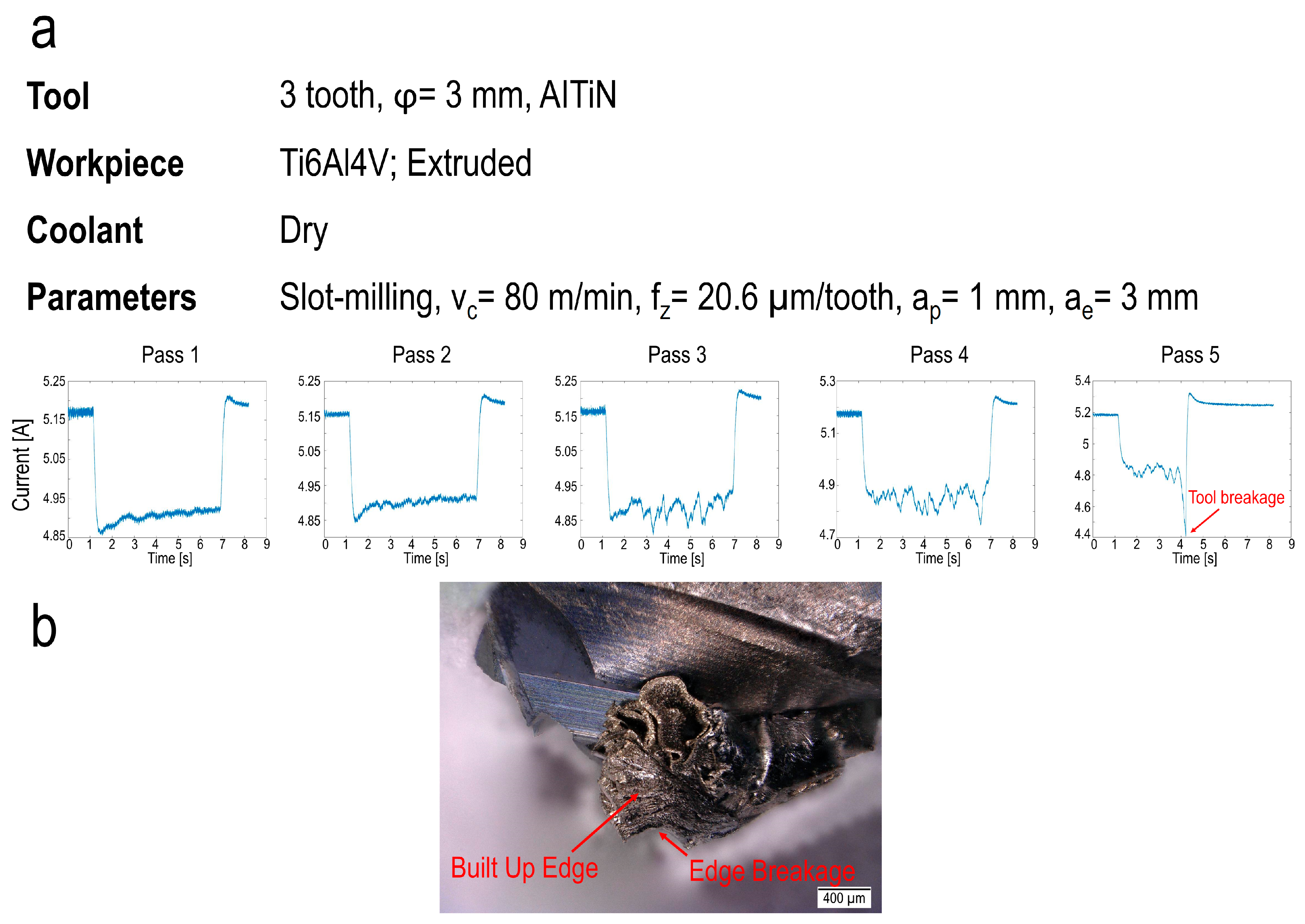
2. Experimental Setup

The milling process used in this experiment was slot milling, and the machined material was Ti6Al4V. Various process parameters were utilized during the milling tests. The axial depth of cut ($a_p$) was set to 1 mm, and the radial depth of cut ($a_e$) was set to 3 mm. The cutting speed ($v_c$) and feed per tooth ($f_z$) were varied in the experiments. Six slot milling passes were performed with and without coolant. The use of coolant prevented tool wear and breakage during the observations. This issue underscores the significant role of cooling as a vital parameter in preventing the onset of critical conditions during machining. The aim of accelerating tool wear and reducing testing duration led to a series of tests conducted without lubrication. These tests included a wide range of feed rates and cutting speeds. In this regard, the mentioned parameters gradually increased to induce the critical conditions.

Table 1. Milling parameters.

Cutting Speed, ${\mathit{v}}_{\mathit{c}}$ (m/min)	Feed Per Tooth, ${\mathit{f}}_{\mathit{z}}$ (μm/tooth)	Radial Depth of Cut, ${\mathit{a}}_{\mathit{e}}$ (mm)	Axial Depth of Cut, ${\mathit{a}}_{\mathit{p}}$ (mm)	Coolant
50–113	17–50	3	1	Oil/Dry

presents the milling parameters.

This study used a five-axis CNC machine tool (Haas-Multigrind^® CA, Trossingen, Germany) with a Siemens Sinumerik controller. The Siemens SINUMERIK EDGE (SE) Box was applied to record data at a resolution of 1 ms (1 kHz). When executing an NC program, the data from different axes of the machine tool were saved in the format of a JSON file. Afterward, ETL (Extract–Transform–Load) program converted the JSON file into a CSV format for each test. After processing the CSV file and extracting useful features, the post-processed information, such as features, was imported into an artificial intelligence (AI) model. Moreover, the machine tool user can then visualize the CSV data from the measurement system on an external computer.

Figure 1a illustrates the experimental setup. As explained, the milling tests were conducted in 6 passes for each test. At each pass, the axial depth of cut, $a_p$, was 1 mm. According to the milling direction shown in Figure 1a, the milling tool moves from the right to the workpiece’s left side. Signals from various machine tool axes were recorded via the SE Box system and saved as a JSON file. Figure 1b illustrates the different axes in the HAAS machine tool. The types of signals that the Edge Box can record for the spindle and each axis are categorized into current, load, torque, and power. The Edge Box starts recording signals automatically before the slot milling process during each milling pass. Similarly, the recording is stopped automatically after the milling process.

Figure 2 illustrates the geometrical characteristics of the milling tool in the study. The utilized tool had a coating of AlTiN. Geometric properties like cutting tool and shank diameter (D1 and D2), total length (L1), cutting edge length (L2), a corner chamfer (EF), and the number of teeth (Z) are provided in the table (See Figure 2).

3. Signal Selection

The previous section mentioned that the data were obtained by extracting signals from JSON files for each experiment. The subsequent phase of the study was allocated to detecting signals that can differentiate between machining and non-machining areas. Moreover, the responsiveness of each signal concerning the variations in machining conditions was evaluated. Among different recorded signals, the current, load, and torque signals in the z-axis meet the pre-defined conditions. They can be used for training the classification model. However, signals from other axes did not display significant changes until the tool failure. Figure 3 illustrates the various types of signals in terms of current, load, power, and torque in the z-axis at a feed speed of 30 µm/tooth and a cutting speed of 50 m/min. Accordingly, the current, load, and torque signals in the z direction reveal the differences between machining and non-machining areas. In contrast, the power signal exhibits no change during the machining.

Figure 4a provides the recorded current signals in the z-axis before the tool breakage. A notable fluctuation in signals is observable after the second pass. This phenomenon can be attributed to the significant Built-Up Edge (BUE) formation, as indicated in Figure 4b, when dry-milling titanium alloys, which ultimately caused tool failure.

As mentioned above, the tool breakage during the experimental tests was considered critical. Additionally, high roughness values of the milled surface were detected as another inappropriate machining condition. Based on these two criteria, the recorded signals were divided into two main groups: safe and critical. The critical group included the signals before the tool breakage and those associated with the high surface roughness values. At the same time, the rest of the signals were related to the safe condition without tool breakage and with appropriate surface quality. Figure 5 indicates the differentiation between these two groups concerning the qualitative and quantitative surface analysis. The critical group highlighted in red exhibits higher surface roughness and low surface quality. In contrast, acceptable surface quality with low surface roughness values can be observed in the safe group. Of the different samples, 726 were classified under the safe group, and the critical group comprised 132.

4. Methods

Figure 6 provides a roadmap of the current research. After data acquisition, the machining time was extracted from the measured signal, and detrended signals were obtained by removing the slope. In order to consider the variations in amplitude caused by different machining parameters in terms of cutting speed and feed per tooth, the signals were normalized using Z-score normalization (Equation (1)). For a fair evaluation of different signals by the statistical features, the signals’ trimming was based on the length of the shortest existing signal. This issue is important because the length of the signal affects several statistical features, thus highlighting the crucial role of uniform signal length. These mentioned steps are explained in the section “Preprocessing Signal”. Next, the feature extraction was performed in three domains (time, frequency, and time–frequency), and the extracted features were concatenated to create a unified primary feature vector. To meet the requirements of machine learning models, where features should have a consistent numerical range, a Z-score normalization was applied to scale the values of the features between 0 and 1. Afterward, a hybrid feature selection technique was employed, combined with simultaneous SVM hyperparameter optimization. This approach, explained in detail in the following sections, aimed to develop a well-trained model capable of accurately classifying the data while identifying the most important features for detecting the machining process conditions.

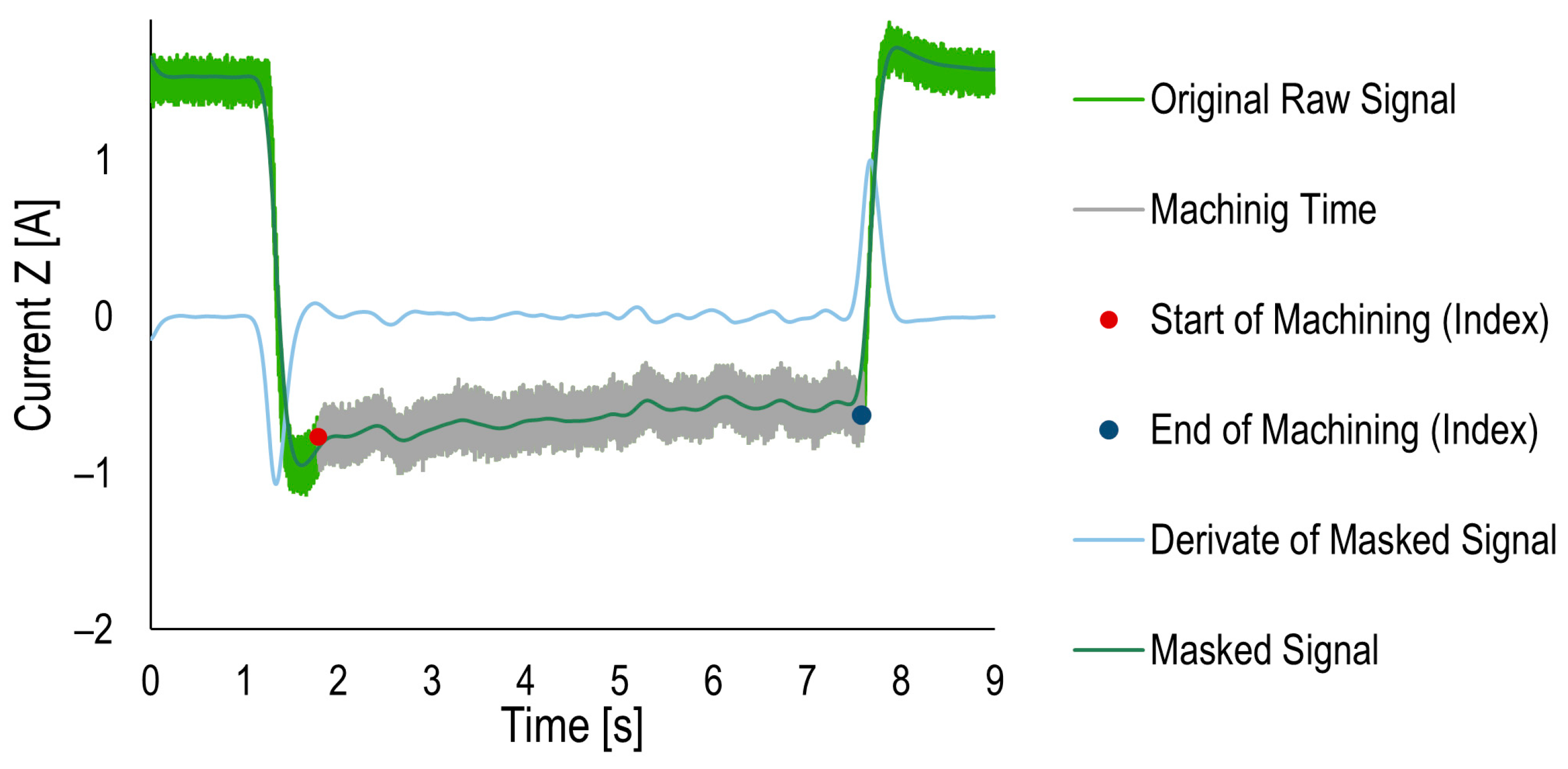
4.1. Preprocessing Signal

As illustrated in Figure 7, before analyzing the signals and extracting their features, the detection of the machining area was conducted. In this regard, the original raw signal (highlighted in green) was subjected to a low-pass filter to remove high-frequency components and form a masked signal (illustrated by dark green color). The derivative of the masked signal indicates one peak and one valley, corresponding to the start and end of the machining time. Consequently, the machining time (highlighted by grey color) was detected concerning these two points.

After detecting the machining time from the entire signal, the extracted signals (corresponding to the machining area) must have the same length because the signal length significantly impacts the statistical features. As mentioned earlier, various tests were conducted at different process parameters regarding cutting speed and feed per tooth, leading to a variation in signal length. To ensure the same signal length from different experimental tests, the smallest signal length was selected as a reference, and the other signals were adjusted by trimming their length, as shown in Figure 8. Additionally, according to Figure 4, it can be observed that the critical condition occurs at the end of each pass. Thus, the uniforming signal length was carried out concerning the signals’ end. Further, the extracted signal was normalized using Equation (1).

$$x_{\mathrm{n}\mathrm{o}\mathrm{r}\mathrm{m}\mathrm{a}\mathrm{l}\mathrm{i}\mathrm{z}\mathrm{e}\mathrm{d}}=\frac{x\left(i\right)-{\overline{x}}_{\mathrm{s}\mathrm{i}\mathrm{g}\mathrm{n}\mathrm{a}\mathrm{l}}}{{\sigma }_{\mathrm{s}\mathrm{i}\mathrm{g}\mathrm{n}\mathrm{a}\mathrm{l}}}$$

(1)

where $x\left(i\right)$, ${\overline{x}}_{\mathrm{s}\mathrm{i}\mathrm{g}\mathrm{n}\mathrm{a}\mathrm{l}}$, and ${\sigma }_{\mathrm{s}\mathrm{i}\mathrm{g}\mathrm{n}\mathrm{a}\mathrm{l}}$ represents the signal points, mean, and standard deviation, respectively. A linear drift was subtracted before normalizing the extracted and trimmed signal. Figure 9 provides the signals in safe and critical conditions after extracting, trimming, detrending, and normalizing. In further steps, these signals were analyzed in different domains discussed in the following sections.

4.2. Signal Analysis

4.2.1. Frequency Domain

Signals were analyzed using the FFT methods. The amplitude of converted signals in the frequency domain was normalized between 0 and 1. Figure 10a,b provide the frequency components of the measured signal in safe and critical conditions, respectively. Accordingly, the amplitude of the frequency components for safe conditions is lower than that for critical conditions at lower frequencies. In detail, the signals associated with the critical condition, which exhibit irregular patterns during metal cutting, lacked periodic variations and demonstrated higher amplitudes near the zero frequency (Figure 10). Upon generating the FFT diagrams for various experimental tests, it was observed that safe and critical signals could be differentiated based on their distinct characteristics across all samples. In order to facilitate this differentiation, the signals were divided into five frequency intervals.

Moreover, the 50 Hz frequency component associated with municipal electricity, which was present in both safe and critical signals, was eliminated from the dataset. Notably, this frequency was removed from all samples in various domains, including frequency, time, and time–frequency domains. As an example, Figure 10c ($v_c$ = 50 m/min and $f_z$ = 30 µm/tooth) and Figure 10d ($v_c$ = 75 m/min and $f_z$ = 22 µm/tooth), respectively, indicate the frequency division; this division was based on the distinguishability of safe and critical signals within the two classes for safe and critical conditions, with the removal of their municipal 50 Hz frequency. Figure 10c,d demonstrate that when the cutting speed increases and critical conditions such as BUE occur, there is a noticeable decrease in the amplitude of the signal in the frequency domain. The wide range of features from frequency components of the signal was extracted in different intervals. As mentioned, feature extraction is explained in Section 4.3.

The findings of this research closely align with the observations made by Tahir et al. [18]. Both studies identified a consistent decrease in the amplitude of the signals in the frequency domain (current signal in this research and main cutting force signal in [18]) as the tool condition deteriorated and the main cutting speed increased. These results further prove the relationship between tool condition, cutting speed, and the corresponding signal amplitudes.

4.2.2. Time Domain

In addition to frequency domain analysis, the preprocessed signals were also analyzed in the time domain. Considering the frequencies discussed earlier in the frequency domain, the time series were divided into five distinct frequency intervals using low-pass, Butterworth, and high-pass filters. This segmentation aimed to differentiate signals from two classes based on their frequency characteristics in the frequency domain, as shown in Figure 10. Moreover, Figure 11 illustrates the signals for safe and critical conditions, respectively. Accordingly, a noticeable distinction between safe and critical signals concerning the signal band at different frequency intervals can be observed. At frequency intervals ranging from 0 to 50 Hz, the signal associated with the critical condition exhibits more fluctuations with sharper edges compared to the safe signals. Therefore, Figure 11 highlights a difference between the signals of safe and critical conditions. In the feature extraction step, these differences are quantified by calculating varied features (See Section 4.3).

4.2.3. Time–Frequency Domain

Wavelets analyze time–frequency traits of signals, decomposing them via a mother wavelet instead of sinusoidal components like the Fourier Transform. Wavelets resemble sinusoids but with a finite duration, existing in both the time and frequency domains [32]. In order to create a family of wavelet functions, a basis function called the mother wavelet, denoted as $\psi \left(t\right)$, is used (Equation (2)) [33].

$${\psi }_{a,\tau }\left(t\right)=\frac{1}{\sqrt{a}}\psi \left(\frac{t-\tau }{a}\right)$$

(2)

The function ${\psi }_{a,\tau }\left(t\right)$ relies on parameters $a$ and $\tau$, determining scale and shift, respectively. In Equation (2), $a<1$ widens the wavelet, and $a>1$ narrows it. $\tau$ shifts $\psi$ along the time axis, while the parameter $a$ changes the scale of $\psi$, which either expands or shortens it. Wavelet is a sliding window on the time axis, convolving with the signal. The process repeats at different scales [34].

Computing the continuous form of the wavelet is a time-consuming task. In order to efficiently analyze the convolution of signals over a wide range of time, it is beneficial to use a discrete form of the Equation. This method incorporates the concepts of scale and shift, as expressed in Equation (3) [35]:

$$a=2^j,\tau ={k2}^j$$

(3)

The process of discrete WT involves the use of a mother wavelet $\psi$, a scaling parameter $j$, and a wavelet transmission variable $k$. When $j$ takes high values, it corresponds to shorter time scales and higher frequencies. The substitution of Equation (3) into Equation (2) results in Equation (4) as the mother wavelet relation. Moreover, the discrete wavelet transfer function is provided in Equation (5) [35]:

$${\psi }_{j,k}=\frac{1}{\sqrt{2^j}}\psi \left(\frac{t-2^{j}k}{2^j}\right)$$

(4)

$$DWT(j,k)=⟨x(t),{\psi }_{j,k}(t)⟩=\frac{1}{\sqrt{2^j}}{\int }_{-\mathrm{\infty }}^{+\mathrm{\infty }}x(t){\psi }^{\mathrm{*}}\left(\frac{t-2^{j}k}{2^j}\right)dt$$

(5)

A filter bank splits a signal into distinct frequencies in practical applications, enabling analysis at various scales. High-pass and low-pass filters evaluate signal frequencies, dividing them into high-frequency details and low-frequency approximations. This decomposition occurs by convolving the wavelet filter and down-sampling, reiterated for each level. Equation (6) reconstructs the original signal via details ($D_i(t)$) and approximations ($A_j(t)$) from discrete wavelet analysis [35].

$$f(t)=\sum _{i=1}^{i=j}{D}_i(t)+A_j(t)$$

(6)

Wavelet tree decomposition involves signal splitting with high-pass and low-pass filters, followed by down-sampling. This iterative process occurs at each wavelet tree level, dividing previous approximations into new details and approximations. This approach allows comprehensive multi-scale signal analysis. This study used the WPD technique to extend filtering to approximation and detail coefficients within the wavelet decomposition tree. This extension captures valuable information from both approximations and details [10,35]. The selection of the mother wavelet depends on the data and the problem. In tool monitoring, the Daubechies function is often used. In this research, the Daubechies 6 wavelet was chosen to analyze current signals and decomposed into five levels (Figure 12). The wavelet type and decomposition levels were determined via trial and error.

4.3. Feature Extraction

Statistical feature extraction was carried out after converting the signals in different domains.

Table 2. Statistical features.

$\mathrm{M}\mathrm{e}\mathrm{a}\mathrm{n}=\frac{{\sum }_{i=1}^{N}x\left(i\right)}{N}$	$\mathrm{E}\mathrm{n}\mathrm{e}\mathrm{r}\mathrm{g}\mathrm{y}={\sum }_{i=1}^N(x(i){)}^2$
$\mathrm{M}\mathrm{a}\mathrm{x}\mathrm{i}\mathrm{m}\mathrm{u}\mathrm{m}=\mathrm{m}\mathrm{a}\mathrm{x}\left(x\right(i\left)\right)$	$\mathrm{K}\mathrm{u}\mathrm{r}\mathrm{t}\mathrm{o}\mathrm{s}\mathrm{i}\mathrm{s}=\frac{\frac{1}{N}{\sum }_{i=1}^N\left(x\right(i)-\overline{x}{)}^4}{\sqrt[\frac{4}{2}]{\frac{1}{N}{\sum }_{i=1}^N\left(x\right(i)-\overline{x}{)}^2}}$
$\mathrm{M}\mathrm{i}\mathrm{n}\mathrm{i}\mathrm{m}\mathrm{u}\mathrm{m}=\mathrm{m}\mathrm{i}\mathrm{n}\left(x\right(i\left)\right)$	$\mathrm{S}\mathrm{k}\mathrm{e}\mathrm{w}\mathrm{n}\mathrm{e}\mathrm{s}\mathrm{s}=\frac{\frac{1}{N}{\sum }_{i=1}^N\left(x\right(i)-\overline{x}{)}^3}{\sqrt[\frac{3}{2}]{\frac{1}{N}{\sum }_{i=1}^N\left(x\right(i)-\overline{x}{)}^2}}$
$\mathrm{P}\mathrm{e}\mathrm{a}\mathrm{k}\mathrm{V}\mathrm{a}\mathrm{l}\mathrm{u}\mathrm{e}=\mathrm{m}\mathrm{a}\mathrm{x}\left(\left|x\left(i\right)\right|\right)$	$\mathrm{R}\mathrm{o}\mathrm{o}\mathrm{t}\mathrm{M}\mathrm{e}\mathrm{a}\mathrm{n}\mathrm{S}\mathrm{q}\mathrm{u}\mathrm{a}\mathrm{r}\mathrm{e}=\sqrt{\frac{{\sum }_{i=1}^N\left(x\right(i){)}^2}{N}}$
$\mathrm{R}\mathrm{a}\mathrm{n}\mathrm{g}\mathrm{e}=\mathrm{m}\mathrm{a}\mathrm{x}\left(x\right)-\mathrm{m}\mathrm{i}\mathrm{n}\left(x\right)$	$\mathrm{L}\mathrm{o}\mathrm{g}\mathrm{E}\mathrm{n}\mathrm{e}\mathrm{r}\mathrm{g}\mathrm{y}\mathrm{E}\mathrm{n}\mathrm{t}\mathrm{r}\mathrm{o}\mathrm{p}\mathrm{y}=-{\sum }_{i=1}^N\left(\mathrm{l}\mathrm{o}{\mathrm{g}}_2\right(p\left(x\right(i\left)\right)){)}^2$
$\mathrm{V}\mathrm{a}\mathrm{r}\mathrm{i}\mathrm{a}\mathrm{n}\mathrm{c}\mathrm{e}=\frac{1}{N}{\sum }_{i=1}^N(x(i)-\overline{x})$	$\mathrm{S}\mathrm{h}\mathrm{a}\mathrm{n}\mathrm{n}\mathrm{o}\mathrm{n}\mathrm{E}\mathrm{n}\mathrm{t}\mathrm{r}\mathrm{o}\mathrm{p}\mathrm{y}=-{\sum }_{i=1}^N\left(p\right(x\left(i\right))\times \mathrm{l}\mathrm{o}{\mathrm{g}}_2\left(p\right(x\left(i\right)\left)\right)$
$\mathrm{S}\mathrm{t}\mathrm{a}\mathrm{n}\mathrm{d}\mathrm{a}\mathrm{r}\mathrm{d}\mathrm{D}\mathrm{e}\mathrm{v}\mathrm{i}\mathrm{a}\mathrm{t}\mathrm{i}\mathrm{o}\mathrm{n}=\sqrt{\frac{{\sum }_{i=1}^N\left(x\right(i)-\overline{x}{)}^2}{N}}$	$\mathrm{H}\mathrm{y}\mathrm{b}\mathrm{r}\mathrm{i}\mathrm{d}\mathrm{F}\mathrm{e}\mathrm{a}\mathrm{t}\mathrm{u}\mathrm{r}\mathrm{e}1=\mathrm{l}\mathrm{o}\mathrm{g}(\mathrm{K}\mathrm{u}\mathrm{r}\mathrm{t}\mathrm{o}\mathrm{s}\mathrm{i}\mathrm{s}+\frac{\mathrm{R}\mathrm{o}\mathrm{o}\mathrm{t}\mathrm{M}\mathrm{e}\mathrm{a}\mathrm{n}\mathrm{S}\mathrm{q}\mathrm{u}\mathrm{a}\mathrm{r}\mathrm{e}}{0.078})$
$\mathrm{G}\mathrm{e}\mathrm{o}\mathrm{m}\mathrm{e}\mathrm{t}\mathrm{r}\mathrm{i}\mathrm{c}\mathrm{M}\mathrm{e}\mathrm{a}\mathrm{n}\mathrm{S}\mathrm{q}\mathrm{u}\mathrm{a}\mathrm{r}\mathrm{e}=({\prod }_{i=1}^N\left|x\left(i\right)\right|{)}^{\frac{1}{N}}$	$\mathrm{T}\mathrm{h}\mathrm{e}\mathrm{A}\mathrm{v}\mathrm{e}\mathrm{r}\mathrm{a}\mathrm{g}\mathrm{e}\mathrm{D}\mathrm{e}\mathrm{v}\mathrm{i}\mathrm{a}\mathrm{t}\mathrm{i}\mathrm{o}\mathrm{n}\mathrm{F}\mathrm{r}\mathrm{o}\mathrm{m}\mathrm{T}\mathrm{h}\mathrm{e}\mathrm{M}\mathrm{e}\mathrm{a}\mathrm{n}={\sum }_{i=1}^N\frac{\left|x\left(i\right)\right|-\overline{x}}{N}$
$\mathrm{Q}\mathrm{u}\mathrm{a}\mathrm{d}\mathrm{r}\mathrm{a}\mathrm{t}\mathrm{i}\mathrm{c}\mathrm{M}\mathrm{e}\mathrm{a}\mathrm{n}\mathrm{S}\mathrm{q}\mathrm{u}\mathrm{a}\mathrm{r}\mathrm{e}={\left(\frac{{\sum }_{i=1}^N\sqrt{\left|\left(x\right(i){)}^2\right|}}{N}\right)}^2$	$\mathrm{T}\mathrm{i}\mathrm{g}\mathrm{e}\mathrm{a}\mathrm{r}-\mathrm{K}\mathrm{a}\mathrm{i}\mathrm{s}\mathrm{e}\mathrm{r}\mathrm{E}\mathrm{n}\mathrm{e}\mathrm{r}\mathrm{g}\mathrm{y}={\displaystyle \sum _{i=1}^N}\left[\right(x\left(i\right){)}^2-x(i-1)x(i+1)]$

displays the utilized features for three domains: time, frequency, and time–frequency. For each milling process, 756 features were extracted: 90 for time (18 features from each frequency band of level 5), 90 for frequency (18 features from each frequency band of level 5), and 576 for time–frequency (18 features from each of the 32 frequency bands of level 5). These features were concatenated for each sample to form a vector of features. Next, a feature matrix was generated with dimensions of 856 × 756, where each row (corresponding to a measured signal (sample)) includes 756 features. The total number of samples accounted for 856. A different range of utilized features can hinder the training and accuracy of machine learning algorithms. The Z-Score method normalized features to address this issue (Equation (1)). Z-Score normalization improves the handling of diverse feature ranges, enhancing training efficiency and accuracy. In Table 2, $x\left(i\right)$ represents the individual signal point, with $i$ ranging from $1$ to $N$, and $p\left(x\right(i\left)\right)$ denotes the probability of each possible value of signal point $x\left(i\right)$. The features highlighted in this article were selected because they are commonly used in condition monitoring based on [12,14,25,27,29,36].

4.4. Feature Selection

Filter and wrapper methods are two approaches in feature selection: selecting a subset of relevant features from a larger set. Filter methods are fast in computation but do not consider the redundancies among features. For example, two features might have very similar statistical measures, such as standard deviation and variance, differing only by a radical in their formulations. Therefore, some of the features may present a high correlation. However, filter methods may still propose both features, even though they are redundant and correlated. This issue can lead to the curse of dimensionality when dealing with many redundant features.

On the other hand, wrapper methods aim to select features that not only differentiate between different classes but also prevent the consideration of redundant features. However, wrapper methods are computationally expensive since they involve evaluating the performance of different feature subsets by training and testing the classification model. A combination of filter and wrapper methods can address the computational cost. This hybrid approach consists of two steps. Firstly, a filter method is applied to eliminate irrelevant features. Then, a wrapper method is used to search for an independent and uncorrelated feature set from the remaining feature set. In the mentioned study, the hybrid approach utilized the t-test as the filter method and the BWOA as the wrapper method.

4.4.1. t-Test

As mentioned, the current study has two safe and critical classes of conditions. The t-test method is used to evaluate the degree of differentiation between the corresponding features of these two classes. Equation (7) provides the calculation of the t-value [37]:

$$t_i=\frac{{\mu }_1-{\mu }_2}{\sqrt{{\left(\frac{{\sigma }_1}{\sqrt{n_1}}\right)}^2+{\left(\frac{{\sigma }_2}{\sqrt{n_2}}\right)}^2}}$$

(7)

where ${\mu }_1$, ${\mu }_2$, ${\sigma }_1$, ${\sigma }_2$, $n_1$ and $n_2$ are the mean of the first class, the mean of the second class, the standard deviation of the first class, the standard deviation of the second class, the number of features in the first class, and the number of features in the second class, respectively. Based on Equation (7), each feature can be evaluated. Accordingly, a lower standard deviation for each class and a higher difference between the means of the two classes results in higher values of t, indicating a better feature for use in the training process. In feature selection for a classification issue, the t-test is used to assess if there is a significant difference between the means of the features in the two classes. For a large number of samples, the t-score follows a normal distribution. If the mean values differ considerably, the feature is considered informative and retained for further analysis or model building. While the t-value in a t-test measures the difference between two groups relative to their variability, the associated p-value, which can be obtained from the related tables or statistical software, indicates the probability of obtaining such a difference by chance alone. This paper set a p-value lower than 0.001 as a threshold for the primary selection of features in the proposed hybrid method [38].

Table 3. Identification of the best features through t-tests across all samples.

t-Test Rank	Domain	Frequency Band (Hz)	Feature Name
1	Time	180–350	Log Energy Entropy
2	Time	180–350	Hybrid Feature 1
3	Frequency	350–500	Mean
4	Frequency	350–500	Hybrid Feature 1
5	Time	180–350	Max

displays the top five features obtained through t-tests conducted on all samples. Accordingly, the log energy entropy feature in the frequency domain with frequency band (180–350 Hz) is considered the most discriminative feature for differentiating these two classes.

Figure 13a presents the normal distribution diagram of log energy entropy for two distinct classes: safe and critical conditions. In order to assess the normality assumption and validate the applicability of the t-test method, a Quantile–Quantile (QQ) plot can be utilized. The QQ plot serves as a graphical tool for comparing the distribution of a dataset to a known theoretical distribution, such as the normal distribution in this case. By plotting the quantiles of the dataset against the quantiles of the theoretical distribution, alignment along a straight line indicates whether the dataset follows the same distribution as the theoretical one. In the context of t-tests, the normality assumption of the data can be verified using the QQ plot. One of the assumptions in conducting a t-test is that the data in each group follows a normal distribution. Suppose the points on the QQ plot closely align with the straight line. In that case, it confirms the data’s approximation using the normal distribution, thus validating the t-test for analysis. As mentioned earlier, the QQ plot in Figure 13b represents the data distribution, specifically the features in each group (safe and critical conditions). A significant difference of points from the straight line suggests a deviation from normally distributed data, indicating the inappropriateness of the t-test for analysis. However, in this case, Figure 13b confirms the applicability of the t-test method as the data points follow the straight line closely, which means that the data in each group is approximately normally distributed.

4.4.2. Whale Optimization Algorithm (WOA)

The Whale algorithm was used in the current investigation to optimize the classification model’s hyperparameters and find the appropriate features. This algorithm consists of two main steps: the exploration phase, where the algorithm searches for prey, and the exploitation phase, where the prey is encircled using a spiral bubble-net feeding maneuver. Whales can detect and trap prey, but the exact location of the prey is often unknown; this algorithm assumes that the best solution is likely near the prey or close to the optimum position of the whale [39].

In the “Exploitation Phase”, the humpback whales (search agents) use Equations (8) and (9) to move closer to the optimal solution when detecting the location of prey [39].

$$\overrightarrow{D}=\left|\overrightarrow{C}\cdot \overrightarrow{X^{\mathrm{*}}}(t)-\overrightarrow{X}\left(t\right)\right|$$

(8)

$$\overrightarrow{X}(t+1)=\overrightarrow{X^{\mathrm{*}}}(t)-\overrightarrow{A}\cdot \overrightarrow{D}$$

(9)

In the current iteration denoted by “$t$”, the coefficient vectors $A$ and $C$ are calculated using Equations (10) and (11). The location vector of the current best whale and the current whale is represented by $X^{*}$ and $X$, respectively. It is important to update $X^{*}$ in every iteration if a better solution or position is found [39]:

$$\overrightarrow{A}=2\cdot \overrightarrow{a}\cdot \overrightarrow{r}-\overrightarrow{a}$$

(10)

$$\overrightarrow{C}=2\cdot \overrightarrow{r}$$

(11)

In each iteration, the value of “$a$” decreases from 2 to 0 according to Equation (12), where “MaxIteration” stands for the highest possible number of iterations. To determine the new location of the whale, random vectors of $r$ are selected within the range of −1 to 1. These values are used to establish the whale’s position between the current best whale and the original location of the whale [40].

$$a=2\left(1-\frac{\mathrm{t}}{\mathrm{M}\mathrm{a}\mathrm{x}\mathrm{I}\mathrm{t}\mathrm{e}\mathrm{r}\mathrm{a}\mathrm{t}\mathrm{i}\mathrm{o}\mathrm{n}}\right)$$

(12)

Two methods are used to model the bubble-net behavior of humpback whales: the shrinking encircling mechanism and spiral updating position. The shrinking encircling mechanism is performed by reducing the value of “$a$” in Equation (10). In the spiral updating position method, Equations (13) and (14) are used to calculate the distance between a whale and its optimal solution, taking into account a spiral pattern similar to the movement of the whale. These Equations can be used to replicate this pattern [39].

$$\overrightarrow{X}(t+1)=\overrightarrow{D\prime }\cdot e^{bl}\cdot \mathrm{c}\mathrm{o}\mathrm{s}(2\pi l)+\overrightarrow{X^{\mathrm{*}}}(t)$$

(13)

$$\overrightarrow{D\prime }=\left|\overrightarrow{X^{\mathrm{*}}}(t)-\overrightarrow{X}\left(t\right)\right|$$

(14)

The distance between the whale and the prey (the best solution obtained so far) is denoted as $D\prime$. The constant value $b$ establishes the shape of the logarithmic spiral that the whale follows around its prey. It is a random number that ranges between 1 and −1 and is used to define the form of that logarithmic spiral. The whale follows a combination of a shrinking encircling path and a spiral path around the prey. Depending on the value of p, the whale algorithm can choose between circular or spiral movements. To simulate this movement, the whale randomly selects either the shrinking encircling path or the spiral path with a 50% probability of updating its position. The model can be represented by Equation (15) [39]:

$$\overrightarrow{X}(t+1)=\left\{\begin{array}{ll}\overrightarrow{X^{\mathrm{*}}}(t)-\overrightarrow{A}\cdot \overrightarrow{D}& \mathrm{i}\mathrm{f} p<0.5\\ \overrightarrow{D\prime }\cdot e^{bl}\cdot \mathrm{c}\mathrm{o}\mathrm{s}(2\pi l)+\overrightarrow{X^{\mathrm{*}}}(t)& \mathrm{i}\mathrm{f} p\ge 0.5\end{array}\right.$$

(15)

where p is a random integer between 0 and 1; whales look for prey randomly in addition to the bubble-net approach. The mathematical model of search is as follows.

In the “Exploration Phase (Search for Prey)”, the search agents focus on broadening the scope of the search and moving away from the previously found solution (rather than relying solely on the best solution). In contrast to the exploitation phase, the exploration phase utilizes random whale selection to update the whale’s position, allowing for more extensive search space exploration. The mathematical model is as follows [39]:

$$\overrightarrow{D}=\left|\overrightarrow{C}\cdot \overrightarrow{X_{rand}}(t)-\overrightarrow{X}(t)\right|$$

(16)

$$\overrightarrow{X}(t+1)=\overrightarrow{X_{rand}}(t)-\overrightarrow{A}\cdot \overrightarrow{D}$$

(17)

In Equations (16) and (17), $X_{rand}$ is a randomly selected whale from the current population. If the absolute number of $\left|A\right|$ is greater than one, a random whale is chosen to update the position of the whales. In contrast, when the absolute number of $\left|A\right|$ is less than one, the best solution is to update the whales’ position. Finally, the whale algorithm terminates by satisfying the termination conditions (maximum iterations).

4.5. Support Vector Machine (SVM)

In a labeled dataset $D$ with $N$ samples, the labels ($y_i$) are binary, having a value of either 1 or −1. The feature vector ($x_i$) is an n-dimensional vector that represents the number of available features and is defined by Equation (18) [41,42].

$$D={\left\{\left(x_i,y_i\right)\left|x_i\in R^n,y_i\in \left\{-\mathrm{1,1}\right\}\right.\right\}}_{i=1}^N$$

(18)

The optimal hyperplane is represented by Equation $f\left(x\right)=\mathit{w}\cdot \mathit{x}+\mathit{b}$, with $\mathit{x}$ as the input, $\mathit{w}$ the feature coefficients, and $b$ as the bias. Solving a convex optimization problem, precisely a quadratic problem, determines this optimal hyperplane. The objective is to minimize ${‖\mathit{w}‖}^2$ while satisfying constraints (Equation (19)), aiming to maximize the margin between the hyperplane and the closest samples from two-class data. The SVM algorithm balances reducing misclassifications and finding a hyperplane with a significant margin, depending on the chosen kernel function (e.g., linear, polynomial, or radial basis function) [12,41].

$$\begin{array}{l}\mathrm{m}\mathrm{i}\mathrm{n}\left(\frac{1}{2}\Vert \mathbf{w}{\Vert }^2+C{\displaystyle \sum _{i=1}^N}{\xi }_i\right)\\ \mathrm{S}\mathrm{u}\mathrm{b}\mathrm{j}\mathrm{e}\mathrm{c}\mathrm{t} \mathrm{t}\mathrm{o}:\left\{\begin{array}{l}{y}_i(\mathbf{w}\cdot \mathbf{x}+b)\ge 1-{\xi }_i\hspace{1em}i=1,\dots ,N\\ {\xi }_i\ge 0\end{array}\right.\end{array}$$

(19)

where ${\xi }_i$ is a slack variable to measure the distance between the hyperplane and misclassified samples, with a penalty coefficient ($C$). The Kuhn–Tucker condition is converted into a dual Lagrangian problem [43] by introducing Lagrangian multipliers for the constraints of the problem (Equation (19)). This problem creates a new quadratic optimization problem. The aim is to measure the difference (${\xi }_i$) between the hyperplane and incorrectly placed samples, and solve the problem using the transformed Lagrangian dual formulation [12,41]:

$$\begin{array}{l}\mathrm{m}\mathrm{i}\mathrm{n}{\displaystyle \sum _{i=1}^{\mathrm{N}}}{\alpha }_i-\frac{1}{2}{\displaystyle \sum _{i=1}^{\mathrm{N}}}{\displaystyle \sum _{j=1}^{\mathrm{N}}}{y}_i{y}_j{\alpha }_i{\alpha }_j{\mathbf{x}}_{\mathbf{i}}{\mathbf{x}}_{\mathbf{j}}\\ \mathrm{S}\mathrm{u}\mathrm{b}\mathrm{j}\mathrm{e}\mathrm{c}\mathrm{t}\mathrm{t}\mathrm{o}:\left\{\begin{array}{l}{\displaystyle \sum _{i=1}^{\mathrm{N}}}{\alpha }_i{y}_i=0\\ 0\le {\alpha }_i\le C\end{array}\right.\end{array}$$

(20)

By solving the optimization problem in Equation (20), the Lagrange coefficient ${\alpha }_i$ (Lagrange coefficient of the $i$-th sample) is determined. This optimal $\alpha$ value is used to calculate the hyperplane parameters ($b$ and $w$), resulting in the following classification function [44]:

$$f(\mathbf{x})=\mathrm{s}\mathrm{i}\mathrm{g}\mathrm{n}\left(\sum _{i=1}^N{\alpha }_i{y}_i\left({\mathbf{x}}_{\mathbf{i}}\cdot {\mathbf{x}}_{\mathbf{j}}\right)+b\right)$$

(21)

When linear separation is impossible, non-linear classification methods like the SVM can be used. By employing a mapping function described in Equation (22), the SVM transfers data from a low-dimensional space to a higher-dimensional space, allowing for easier separation between class borders. Equation (23) introduces the use of a non-linear function, $\varphi \left(\mathbf{x}\right)$, to map input feature vectors ($x_i$) from an $n$-dimensional space to an $l$-dimensional feature space, enhancing classification. This problem requires defining the kernel function $K\left({\mathbf{x}}_{\mathbf{i}},{\mathbf{x}}_{\mathbf{j}}\right)$, as specified in Equation (24) [44].

$$\forall i,x_i\to \phi \left(x_i\right)$$

(22)

$$\varphi \left(\mathbf{x}\right)=\left({\phi }_1\left(\mathbf{x}\right),\dots ,{\phi }_l\left(\mathbf{x}\right)\right)$$

(23)

$$K\left({\mathbf{x}}_{\mathbf{i}},{\mathbf{x}}_{\mathbf{j}}\right)=\left(\varphi \left({\mathbf{x}}_{\mathbf{i}}\right)\cdot \varphi \left({\mathbf{x}}_{\mathbf{j}}\right)\right)$$

(24)

Subsequently, the optimization problem can be converted into the equation expressed as follows [41]:

$$\begin{array}{l}\mathrm{m}\mathrm{i}\mathrm{n}{\displaystyle \sum _{i=1}^{\mathrm{N}}}{\alpha }_i-\frac{1}{2}{\displaystyle \sum _{i=1}^{\mathrm{N}}}{\displaystyle \sum _{j=1}^{\mathrm{N}}}{y}_i{y}_j{\alpha }_i{\alpha }_{j}K\left({\mathbf{x}}_{\mathbf{i}},{\mathbf{x}}_{\mathbf{j}}\right)\\ \mathrm{S}\mathrm{u}\mathrm{b}\mathrm{j}\mathrm{e}\mathrm{c}\mathrm{t} \mathrm{t}\mathrm{o}:\left\{\begin{array}{l}{\displaystyle \sum _{i=1}^{\mathrm{N}}}{\alpha }_i{y}_i=0\\ 0\le {\alpha }_i\le C\end{array}\right.\end{array}$$

(25)

When the non-linear kernel is used, Equation (21) for the decision function is modified and transformed into Equation (26) [44].

$$f(\mathbf{x})=\mathrm{s}\mathrm{i}\mathrm{g}\mathrm{n}\left(\sum _{i,j=1}^N{\alpha }_i{y}_{i}K\left({\mathbf{x}}_{\mathbf{i}},{\mathbf{x}}_{\mathbf{j}}\right)+b\right)$$

(26)

The radial basis function is a commonly used kernel in SVM applications. It is defined as Equation (27) [12]:

$$K\left({\mathbf{x}}_{\mathbf{i}}\cdot {\mathbf{x}}_{\mathbf{j}}\right)=\mathrm{e}\mathrm{x}\mathrm{p}\left(-\frac{{‖{\mathbf{x}}_{\mathbf{i}}-{\mathbf{x}}_{\mathbf{j}}‖}^2}{{\sigma }^2}\right)$$

(27)

SVMs are well known for their computational efficiency and effectiveness in handling high-dimensional data without relying on complex models. This advantage arises from their unique ability to overcome the “curse of dimensionality”, allowing them to navigate such spaces without being overwhelmed by excessive parameters. However, SVMs lack an efficient method for selecting the optimal kernel function, making it a challenging research problem. Choosing kernel parameters, such as $\sigma$ and $C$, is crucial for optimizing the classifier’s error performance. Hyperparameters, such as $C$ and $\sigma$, are vital in determining how well the classifier generalizes to new data beyond the training set. Proper tuning of these hyperparameters significantly influences the overall effectiveness of SVMs. Despite this challenge, SVMs achieve superior generalization performance, ranking at the top in studies comparing them to other classifiers [38]. This study utilizes the whale optimization algorithm to find the optimal values for these parameters.

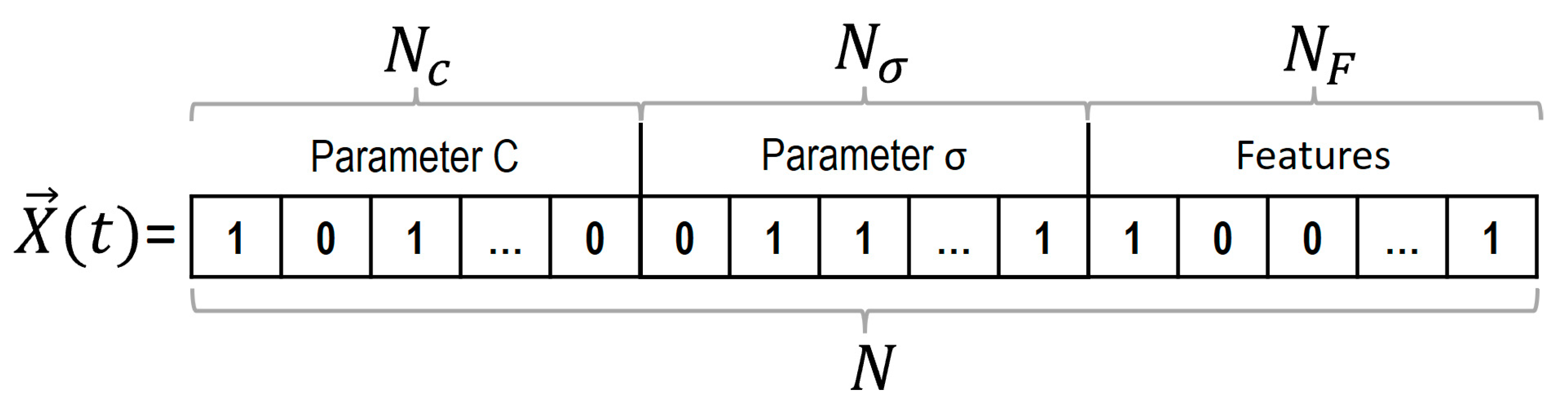
4.6. Encoding and WOA Parameters

According to Figure 14, the whale’s position $\overrightarrow{X}(t)$ includes three main sections of $N_c$, $N_{\sigma }$, and $N_F$. To create the vector of the whale’s position, the values of parameters $C$ and $\sigma$ associated with hyperparameters of the SVM classification method are converted into the binary values (0 and 1) and stored in sections $N_c$ and $N_{\sigma }$, respectively. Moreover, $N_F$ determines the state of the features (active or inactive), according to Equations (28) and (29):

$$\overrightarrow{X_{ij}}=\left\{\begin{array}{ll}1,& \mathrm{i}\mathrm{f} sigmoid\left(\overrightarrow{X_{ij}}\right)\ge \mathrm{r}\mathrm{a}\mathrm{n}\mathrm{d}()\\ 0,& \mathrm{o}\mathrm{t}\mathrm{h}\mathrm{e}\mathrm{r}\mathrm{w}\mathrm{i}\mathrm{s}\mathrm{e}\end{array}\right.$$

(28)

$$sigmoid(\overrightarrow{X_{ij}})=\frac{1}{1+e^{-10(\overrightarrow{X_{ij}}-0.5)}}$$

(29)

In Equation (28), $\overrightarrow{X_{ij}}$ represents the $j$-th dimension for the $i$-th whale. A comparison between the sigmoid function and the generated random variable determines whether a 0 or 1 value is assigned to the corresponding dimension [45,46]. The acceptable ranges [$x_{dmin}$, $x_{dmax}$] for $C$ and $\sigma$, specified by Chegini et al. [12], are [0.001, 100] and [0.01, 10], respectively. In this regard, the process of debinarization of $C$ and $\sigma$ values into the demical ones can be carried out using Equation (30).

$$x_d=\frac{\sum _{i=1}^N\left(\mathrm{b}\mathrm{i}\mathrm{t}\left(i\right)\cdot 2^i\right)}{2^N-1}\left(x_{dmax}-x_{\mathit{dmin}}\right)+x_{\mathit{dmin}}$$

(30)

For each of these whale positions, the cost of the proposed position is calculated through Equation (36).

The range of values for the BWOA algorithm parameters and the $C$ and $\sigma$ parameters are first determined. The BWOA algorithm uses a population of whales, with nPop = 20 whales and MaxIt = 1000 maximum iterations.

5. Results and Discussion

When evaluating a classification model, various factors come into play: accuracy, precision, recall, specificity, and geometric mean. In order to assess these factors, a confusion matrix (

Table 4. Confusion matrix.

	$\mathbf{P}\mathbf{o}\mathbf{s}\mathbf{i}\mathbf{t}\mathbf{i}\mathbf{v}\mathbf{e} \mathbf{P}\mathbf{r}\mathbf{e}\mathbf{d}\mathbf{i}\mathbf{c}\mathbf{t}\mathbf{i}\mathbf{o}\mathbf{n}$	$\mathbf{N}\mathbf{e}\mathbf{g}\mathbf{a}\mathbf{t}\mathbf{i}\mathbf{v}\mathbf{e} \mathbf{P}\mathbf{r}\mathbf{e}\mathbf{d}\mathbf{i}\mathbf{c}\mathbf{t}\mathbf{i}\mathbf{o}\mathbf{n}$
$\mathrm{P}\mathrm{o}\mathrm{s}\mathrm{i}\mathrm{t}\mathrm{i}\mathrm{v}\mathrm{e} \mathrm{C}\mathrm{l}\mathrm{a}\mathrm{s}\mathrm{s}$	$\mathrm{T}\mathrm{r}\mathrm{u}\mathrm{e} \mathrm{P}\mathrm{o}\mathrm{s}\mathrm{i}\mathrm{t}\mathrm{i}\mathrm{v}\mathrm{e} \left(\mathrm{T}\mathrm{P}\right)$	$\mathrm{F}\mathrm{a}\mathrm{l}\mathrm{s}\mathrm{e} \mathrm{N}\mathrm{e}\mathrm{g}\mathrm{a}\mathrm{t}\mathrm{i}\mathrm{v}\mathrm{e} \left(\mathrm{F}\mathrm{N}\right)$
$\mathrm{N}\mathrm{e}\mathrm{g}\mathrm{a}\mathrm{t}\mathrm{i}\mathrm{v}\mathrm{e} \mathrm{C}\mathrm{l}\mathrm{a}\mathrm{s}\mathrm{s}$	$\mathrm{F}\mathrm{a}\mathrm{l}\mathrm{s}\mathrm{e} \mathrm{P}\mathrm{o}\mathrm{s}\mathrm{i}\mathrm{t}\mathrm{i}\mathrm{v}\mathrm{e} \left(\mathrm{F}\mathrm{P}\right)$	$\mathrm{T}\mathrm{r}\mathrm{u}\mathrm{e} \mathrm{N}\mathrm{e}\mathrm{g}\mathrm{a}\mathrm{t}\mathrm{i}\mathrm{v}\mathrm{e} \left(\mathrm{T}\mathrm{N}\right)$

) is constructed for each set of test cases. In binary classification, this matrix consists of four outcomes: true positive, true negative, false positive, and false negative. A true positive occurs when the model correctly identifies positive samples. In contrast, a true negative happens when it correctly identifies negative samples.

Conversely, false positives and false negatives occur when the model mistakenly labels samples as positive or negative. The model’s performance is evaluated by computing metrics involving true positive, true negative, false positive, and false negative. The confusion matrix visually represents the model’s performance, with rows indicating actual classes and columns representing predicted classes.

Accuracy reflects the overall correctness of the model. It is calculated by dividing the number of correctly predicted samples by the total number of samples in the confusion matrix (See Equation (31)). According to Equation (32), precision, on the other hand, evaluates the accuracy of positive sample labeling. It is determined by dividing the number of true positive samples by the total number of samples predicted as positive. Recall, also known as sensitivity or true positive rate, focuses on the ability of the model to correctly identify positive samples, as provided in Equation (33). It is computed by dividing the number of true positive samples by the total number of actual positive samples. Specificity, also called the true negative rate, measures the capability of the model to identify negative samples correctly. As indicated in Equation (34), it is calculated by dividing the number of true negative samples by the total number of actual negative samples. The geometric mean in Equation (35) combines accuracy and recall, providing insights into the balance between majority and minority groups. This criterion proves particularly useful in specific classification problems [47].

$$Accuracy=\frac{TP+TN}{TP+TN+FP+FN}$$

(31)

$$Precision=\frac{TP}{TP+FP}$$

(32)

$$Recall=\frac{TP}{TP+FN}$$

(33)

$$Specificity=\frac{TN}{TN+FP}$$

(34)

$$G-Mean=\sqrt{\frac{TP}{TP+FN}\times \frac{TN}{TN+FP}}=\sqrt{\mathrm{S}\mathrm{p}\mathrm{e}\mathrm{c}\mathrm{i}\mathrm{f}\mathrm{i}\mathrm{c}\mathrm{i}\mathrm{t}\mathrm{y}\times \mathrm{S}\mathrm{e}\mathrm{n}\mathrm{s}\mathrm{i}\mathrm{t}\mathrm{i}\mathrm{v}\mathrm{i}\mathrm{t}\mathrm{y}}$$

(35)

The accuracy criterion is commonly employed to evaluate the performance of the model. It is also often incorporated into the cost function of wrapper methods. However, it may not be an appropriate measure for evaluating the model’s performance when the dataset is imbalanced. In an imbalanced dataset, the minority (Critical) group is neglected, as its size is significantly smaller than the majority (Safe) group. The current study followed the method employed in [47]. It incorporated the geometric mean into the cost function instead of relying on accuracy as a measure in an imbalanced dataset. This modification was necessary because the geometric mean relationship is more effective than the accuracy criterion for evaluating models in imbalanced datasets.

During the optimization process, each position of the whale is evaluated using the cost function (Equation (36)), which comprises the prediction error and the number of selected features:

$$\mathrm{C}\mathrm{o}\mathrm{s}\mathrm{t}\mathrm{F}\mathrm{u}\mathrm{n}\mathrm{c}\mathrm{t}\mathrm{i}\mathrm{o}\mathrm{n}=\alpha \times (1-\sqrt{\mathrm{S}\mathrm{p}\mathrm{e}\mathrm{c}\mathrm{i}\mathrm{f}\mathrm{i}\mathrm{c}\mathrm{i}\mathrm{t}\mathrm{y}\times \mathrm{S}\mathrm{e}\mathrm{n}\mathrm{s}\mathrm{i}\mathrm{t}\mathrm{i}\mathrm{v}\mathrm{i}\mathrm{t}\mathrm{y}})+(1-\alpha )\times (\frac{\mathrm{N}\mathrm{u}\mathrm{m}\mathrm{b}\mathrm{e}\mathrm{r} \mathrm{o}\mathrm{f} \mathrm{S}\mathrm{e}\mathrm{l}\mathrm{e}\mathrm{c}\mathrm{t}\mathrm{e}\mathrm{d} \mathrm{F}\mathrm{e}\mathrm{a}\mathrm{t}\mathrm{u}\mathrm{r}\mathrm{e}\mathrm{s}}{\mathrm{T}\mathrm{o}\mathrm{t}\mathrm{a}\mathrm{l} \mathrm{N}\mathrm{u}\mathrm{m}\mathrm{b}\mathrm{e}\mathrm{r} \mathrm{o}\mathrm{f} \mathrm{F}\mathrm{e}\mathrm{a}\mathrm{t}\mathrm{u}\mathrm{r}\mathrm{e}\mathrm{s}})$$

(36)

The weight coefficient of this study ($\alpha$) is set to 0.01, the same value used in a reference [12]. The first term of Equation (36) measures the error, which refers to the geometric mean difference from one in the validation dataset. The purpose of this cost function is to balance the tradeoff between the error rate and the number of selected features using the alpha coefficient.

In this study, the performance of SVM classification was enhanced by employing the hybrid t-test and the BWOA feature selection method. The data were divided into twenty groups using K-fold cross-validation (Figure 15). Five folds were assigned for training, validation, and testing. The hybrid method utilized four folds (training and validation) for feature selection and optimization of the SVM hyperparameters in this framework. In contrast, one fold was exclusively reserved for testing the model. This iterative process was repeated twenty times to encompass all possible combinations [48]. The mean and standard deviation of performance were calculated across the 20 testing sets. Each sample comprised 726 features from two classes. The t-test method was employed to select the most discriminative features, with an average of 527 features surpassing the p-value significance level of 0.001 [38], facilitating the removal of features with inadequate resolution.

Table 5. Performance of the testing dataset (mean ± standard deviation).

Total Selected Features	Validation Accuracy	Validation Precision	Validation Recall	Validation Specificity
	99.36 ± 0.78	99.60 ± 1.23	96.27 ± 5.06	99.93 ± 0.21
16.45 ± 6.06	Test Accuracy	Test Precision	Test Recall	Test Specificity
	94.84 ± 1.43	85.55 ± 6.79	79.89 ± 7.69	97.52 ± 1.13
	Caverage	σaverage	CBest fold	σBest fold
	41.75 ± 23.19	5.41 ± 1.32	75.39 ± 0	5.04 ± 0

and Figure 16 summarize the outcomes obtained from the training and testing of these groups.

The study focused exclusively on identifying the features that demonstrated the highest performance on the test data within a specific fold. The Tiger Kaiser energy feature of the wavelet coefficient consistently appeared in multiple folds, including the best one, with a bandwidth ranging from 0 to 15.6 Hz. Additionally, several other features considered adequate due to their frequent repetition across different folds are indicated in

Table 6. Identifying best features using the t-test and the BWOA with the highest repetition across 20 folds.

Number	Number of Repetitions across 20 Folds	Domain	Frequency Band (Hz)	Feature Name
1	9	Time–Frequency	0–15.6	Teager Kaiser
2	8	Frequency	350–500	Teager Kaiser
3	5	Time–Frequency	78.1–93.7	Log Energy Entropy
4	4	Time–Frequency	359.3–375	Range
5	3	Frequency	350–500	Log Energy Entropy

.

6. Conclusions

This study was allocated to predict critical machining conditions for Ti6Al4V as a difficult-to-cut material. The process signals were collected using the Siemens SINUMERIK Edge (SE) Box during slot milling. To select the most suitable features from measured signals, a hybrid method, combining the t-test and the BWOA, was applied to train the SVM classification model and select valuable features. Additionally, the parameters of the SVM model were simultaneously updated during the feature selection process. Overall, the findings of this study indicated great potential for monitoring and predicting critical machining conditions during the slot milling of Ti6Al4V. In summary, the results of this investigation are as follows:

Among different measured signals, the signals in the z-direction for current, load, and torque indicated better differentiation between non-machining and machining time.

The validation of the SVM indicated an accuracy of 99.36 ± 0.78%, a precision of 99.60 ± 1.23%, a recall of 96.27 ± 5.06%, and a specificity of 99.93 ± 0.21%.

In the testing phase, the model showed an accuracy of 94.84 ± 1.43%, a precision of 85.55 ± 6.79%, a recall of 79.89 ± 7.69%, and a specificity of 97.52 ± 1.13%.

Using the t-test and the BWOA, the important features were Teager Kaiser, log energy entropy, and range found in frequency and time–frequency domains.

Overall, the model performed well in validation and test sets, indicating that the feature selection process successfully identified important features for the classification task. The findings of this study show great potential for monitoring and predicting critical milling conditions during the slot milling of Ti6Al4V.

This research highlights the importance of data-driven machining in the fourth industrial revolution, focusing on its effectiveness in predicting machining conditions. Unlike traditional simulation models that heavily rely on approximations and assumptions, data-driven methods utilize real-time data from machining sensors, enabling precise predictions. This methodology leads to improved productivity, reduced waste, and better decision making. This approach can also be applied to various manufacturing processes.

References

1. Michelsen, K.-E. Industry 4.0 in Retrospect and in Context. In Technical, Economic and Societal Effects of Manufacturing 4.0; IDEAS: Paris, France, 2020; pp. 1–14. [Google Scholar]
2. Oztemel, E.; Gursev, S. Literature review of Industry 4.0 and related technologies. J. Intell. Manuf. 2020, 31, 127–182. [Google Scholar] [CrossRef]
3. Bajaj, N.S.; Patange, A.D.; Jegadeeshwaran, R.; Pardeshi, S.S.; Kulkarni, K.A.; Ghatpande, R.S. Application of metaheuristic optimization based support vector machine for milling cutter health monitoring. Intell. Syst. Appl. 2023, 18, 200196. [Google Scholar] [CrossRef]
4. He, Z.; Shi, T.; Xuan, J.; Li, T. Research on tool wear prediction based on temperature signals and deep learning. Wear 2021, 478–479, 203902. [Google Scholar] [CrossRef]
5. Polini, W.; Turchetta, S. Cutting force, tool life and surface integrity in milling of titanium alloy Ti-6Al-4V with coated carbide tools. Proc. Inst. Mech. Eng. Part B J. Eng. Manuf. 2016, 230, 694–700. [Google Scholar] [CrossRef]
6. Aghazadehkouzekonani, F. A Contribution to Online Tool Wear Detection Using Deep Learning Methodology. Ph.D. Thesis, École de Technologie Supérieure, Montréal, QC, Canada, 2020. [Google Scholar]
7. Zhu, K.P.; Wong, Y.S.; Hong, G.S. Wavelet analysis of sensor signals for tool condition monitoring: A review and some new results. Int. J. Mach. Tools Manuf. 2009, 49, 537–553. [Google Scholar] [CrossRef]
8. Pimenov, D.Y.; Kumar Gupta, M.; da Silva, L.R.R.; Kiran, M.; Khanna, N.; Krolczyk, G.M. Application of measurement systems in tool condition monitoring of Milling: A review of measurement science approach. Meas. J. Int. Meas. Confed. 2022, 199, 111503. [Google Scholar] [CrossRef]
9. Liu, M.K.; Tseng, Y.H.; Tran, M.Q. Tool wear monitoring and prediction based on sound signal. Int. J. Adv. Manuf. Technol. 2019, 103, 3361–3373. [Google Scholar] [CrossRef]
10. García Plaza, E.; Núñez López, P.J. Application of the wavelet packet transform to vibration signals for surface roughness monitoring in CNC turning operations. Mech. Syst. Signal Process. 2018, 98, 902–919. [Google Scholar] [CrossRef]
11. Segreto, T.; D’Addona, D.; Teti, R. Tool wear estimation in turning of Inconel 718 based on wavelet sensor signal analysis and machine learning paradigms. Prod. Eng. 2020, 14, 693–705. [Google Scholar] [CrossRef]
12. Nezamivand Chegini, S.; Bagheri, A.; Najafi, F. A new intelligent fault diagnosis method for bearing in different speeds based on the FDAF-score algorithm, binary particle swarm optimization, and support vector machine. Soft Comput. 2020, 24, 10005–10023. [Google Scholar] [CrossRef]
13. Han, Z.; Zhang, X.; Yan, B.; Qiao, L.; Wang, Z. The time-frequency analysis of the acoustic signal produced in underwater discharges based on Variational Mode Decomposition and Hilbert–Huang TransforQm. Sci. Rep. 2023, 13, 22. [Google Scholar] [CrossRef] [PubMed]
14. Hu, M.; Ming, W.; An, Q.; Chen, M. Tool wear monitoring in milling of titanium alloy Ti–6Al–4 V under MQL conditions based on a new tool wear categorization method. Int. J. Adv. Manuf. Technol. 2019, 104, 4117–4128. [Google Scholar] [CrossRef]
15. Li, X.; Dong, S.; Yuan, Z. Discrete wavelet transform for tool breakage monitoring. Int. J. Mach. Tools Manuf. 1999, 39, 1935–1944. [Google Scholar] [CrossRef]
16. Li, G.; Yang, X.; Chen, D.; Song, A.; Fang, Y.; Zhou, J. Tool breakage detection using deep learning. In Proceedings of the 2018 IEEE/ACIS 3rd International Conference on Big Data, Cloud Computing, Data Science and Engineering, BCD 2018, Yonago, Japan, 12–13 July 2018; IEEE: New York, NY, USA, 2018; pp. 37–42. [Google Scholar]
17. Kolar, P.; Burian, D.; Fojtu, P.; Masek, P.; Fiala, S.; Chladek, S.; Petracek, P.; Sveda, J.; Rytir, M. Indirect Drill Condition Monitoring Based on Machine Tool Control System Data. MM Sci. J. 2022, 2022-Octob, 5905–5912. [Google Scholar] [CrossRef]
18. Tahir, N.H.M.; Muhammad, R.; Ghani, J.A.; Nuawi, M.Z.; Haron, C.H.C. Monitoring the flank wear using piezoelectric of rotating tool of main cutting force in end milling. J. Teknol. 2016, 78, 45–51. [Google Scholar] [CrossRef]
19. Aghazadeh, F.; Tahan, A.; Thomas, M. Tool condition monitoring using spectral subtraction and convolutional neural networks in milling process. Int. J. Adv. Manuf. Technol. 2018, 98, 3217–3227. [Google Scholar] [CrossRef]
20. Niaki, F.A.; Ulutan, D.; Mears, L. Wavelet based sensor fusion for tool condition monitoring of hard to machine materials. In Proceedings of the 2015 IEEE International Conference on Multisensor Fusion and Integration for Intelligent, San Diego, CA, USA, 14–16 September 2015; pp. 271–276. [Google Scholar]
21. Hojati, F.; Azarhoushang, B.; Daneshi, A.; Hajyaghaee Khiabani, R. Prediction of Machining Condition Using Time Series Imaging and Deep Learning in Slot Milling of Titanium Alloy. J. Manuf. Mater. Process. 2022, 6, 145. [Google Scholar] [CrossRef]
22. Pagani, L.; Parenti, P.; Cataldo, S.; Scott, P.J.; Annoni, M. Indirect cutting tool wear classification using deep learning and chip colour analysis. Int. J. Adv. Manuf. Technol. 2020, 111, 1099–1114. [Google Scholar] [CrossRef]
23. Tabakhi, S.; Moradi, P. Relevance-redundancy feature selection based on ant colony optimization. Pattern Recognit. 2015, 48, 2798–2811. [Google Scholar] [CrossRef]
24. Nouri-Moghaddam, B.; Ghazanfari, M.; Fathian, M. A novel bio-inspired hybrid multi-filter wrapper gene selection method with ensemble classifier for microarray data. In Neural Computing and Applications; Springer: London, UK, 2021; Volume 9. [Google Scholar] [CrossRef]
25. Kusy, M.; Zajdel, R.; Kluska, J.; Zabinski, T. Fusion of Feature Selection Methods for Improving Model Accuracy in the Milling Process Data Classification Problem. In Proceedings of the 2020 International Joint Conference on Neural Networks, Glasgow, UK, 19–24 July 2020. [Google Scholar]
26. Xie, Z.; Li, J.; Lu, Y. Feature selection and a method to improve the performance of tool condition monitoring. Int. J. Adv. Manuf. Technol. 2019, 100, 3197–3206. [Google Scholar] [CrossRef]
27. Liao, X.; Zhou, G.; Zhang, Z.; Lu, J.; Ma, J. Tool wear state recognition based on GWO–SVM with feature selection of genetic algorithm. Int. J. Adv. Manuf. Technol. 2019, 104, 1051–1063. [Google Scholar] [CrossRef]
28. Chen, Y.; Li, H.; Hou, L.; Wang, J.; Bu, X. An intelligent chatter detection method based on EEMD and feature selection with multi-channel vibration signals. Meas. J. Int. Meas. Confed. 2018, 127, 356–365. [Google Scholar] [CrossRef]
29. Binsaeid, S.; Asfour, S.; Cho, S.; Onar, A. Machine ensemble approach for simultaneous detection of transient and gradual abnormalities in end milling using multisensor fusion. J. Mater. Process. Technol. 2009, 209, 4728–4738. [Google Scholar] [CrossRef]
30. Kossakowska, J.; Bombiński, S.; Ejsmont, K. Analysis of the suitability of signal features for individual sensor types in the diagnosis of gradual tool wear in turning. Energies 2021, 14, 6489. [Google Scholar] [CrossRef]
31. Lei, Z.; Zhu, Q.; Zhou, Y.; Sun, B.; Sun, W.; Pan, X. A GAPSO-Enhanced Extreme Learning Machine Method for Tool Wear Estimation in Milling Processes Based on Vibration Signals. Int. J. Precis. Eng. Manuf. Green Technol. 2021, 8, 745–759. [Google Scholar] [CrossRef]
32. García Plaza, E.; Núñez López, P.J. Analysis of cutting force signals by wavelet packet transform for surface roughness monitoring in CNC turning. Mech. Syst. Signal Process. 2018, 98, 634–651. [Google Scholar] [CrossRef]
33. Khazaee, M.; Banakar, A.; Ghobadian, B.; Agha Mirsalim, M.; Minaei, S.; Jafari, S.M. Detection of inappropriate working conditions for the timing belt in internal-combustion engines using vibration signals and data mining. Proc. Inst. Mech. Eng. Part D J. Automob. Eng. 2017, 231, 418–432. [Google Scholar] [CrossRef]
34. Avijit Chakraborty, D.O. Frequency-time decomposition of seismic data using wavelet-based methods. Geophysics 1995, 60, 1058–1065. [Google Scholar] [CrossRef]
35. Khazaee, M.; Ahmadi, H.; Omid, M.; Banakar, A.; Moosavian, A. Feature-level fusion based on wavelet transform and artificial neural network for fault diagnosis of planetary gearbox using acoustic and vibration signals. Insight Non-Destr. Test. Cond. Monit. 2013, 55, 323–330. [Google Scholar] [CrossRef]
36. Moosavian, A.; Ahmadi, H.; Tabatabaeefar, A.; Khazaee, M. Comparison of two classifiers; K-nearest neighbor and artificial neural network, for fault diagnosis on a main engine journal-bearing. Shock Vib. 2013, 20, 263–272. [Google Scholar] [CrossRef]
37. Potochnik, A.; Colombo, M.; Wright, C. Statistics and Probability. Recipes Sci. 2018, 167–206. [Google Scholar]
38. Theodoridis, S.; Koutroumbas, K. Pattern Recognition; Elsevier: Amsterdam, The Netherlands, 2009; pp. 1–967. Available online: https://darmanto.akakom.ac.id/pengenalanpola/PatternRecognition4thEd.(2009).pdf (accessed on 11 August 2022). [CrossRef]
39. Mirjalili, S.; Lewis, A. The Whale Optimization Algorithm. Adv. Eng. Softw. 2016, 95, 51–67. [Google Scholar] [CrossRef]
40. Mafarja, M.; Mirjalili, S. Whale optimization approaches for wrapper feature selection. Appl. Soft Comput. 2018, 62, 441–453. [Google Scholar] [CrossRef]
41. Haykin, S. Neural Networks and Learning Machines, 3rd ed.; Pearson Education India: Delhi, India, 2009. [Google Scholar]
42. Vapnik, V.N. The Nature of Statistical Learning Theory; Springer: New York, NY, USA, 2000. [Google Scholar]
43. Nezamivand Chegini, S.; Amini, P.; Ahmadi, B.; Bagheri, A.; Amirmostofian, I. Intelligent bearing fault diagnosis using swarm decomposition method and new hybrid particle swarm optimization algorithm. Soft Comput. 2022, 26, 1475–1497. [Google Scholar] [CrossRef]
44. Nezamivand, C.S.; Bagheri, A.; Najafi, F. A New Hybrid Intelligent Technique Based on Improving the Compensation Distance Evaluation Technique and Support Vector Machine for Bearing Fault Diagnosis. Modares Mech. Eng. 2019, 19, 865–875. [Google Scholar]
45. Eid, H.F. Binary whale optimisation: An effective swarm algorithm for feature selection. Int. J. Metaheuristics 2018, 7, 67. [Google Scholar] [CrossRef]
46. Xu, H.; Fu, Y.; Fang, C.; Cao, Q.; Su, J.; Wei, S. An improved binary whale optimization algorithm for feature selection of network intrusion detection. In Proceedings of the 2018 IEEE 4th International Symposium on Wireless Systems within the International Conferences on Intelligent Data Acquisition and Advanced Computing Systems, IDAACS-SWS 2018, Lviv, Ukraine, 20–21 September 2018; IEEE: New York, NY, USA, 2018; pp. 10–15. [Google Scholar]
47. Da Li, A.; Xue, B.; Zhang, M. Multi-objective feature selection using hybridization of a genetic algorithm and direct multisearch for key quality characteristic selection. Inf. Sci. 2020, 523, 245–265. [Google Scholar]
48. Abdar, A.K.; Sadjadi, S.M.; Bashirgonbadi, A.; Naghibi, M.; Soltanian-Zadeh, H. Extended VGG16 Deep-Learning Detects COVID-19 from Chest CT Images. AUT J. Electr. Eng. 2022, 54, 79–90. [Google Scholar]
Figure 1. (a) Experimental setup; (b) illustration of the different axes.
Machines 11 00835 g001
Figure 2. Geometrical characteristics of the utilized cutting tool manufactured by HB microtec GmbH & Co. KG, Germany.
Machines 11 00835 g002
Figure 3. Current, load, power, and torque signals from the z-axis at 50 m/min cutting speed and 30 µm/tooth feed.
Machines 11 00835 g003
Figure 4. (a) Signals of current in different passes before tool breakage at v c = 80 m/min and f z = 20.6 µm/tooth, and (b) BUE and edge chipping at v c = 80 m/min and f z = 20.6 µm/tooth.
Machines 11 00835 g004
Figure 5. Grouping the samples concerning the quantitative and qualitative analysis.
Machines 11 00835 g005
Figure 6. The roadmap of the current research.
Machines 11 00835 g006
Figure 7. Detection of the machining area.
Machines 11 00835 g007
Figure 8. (a) Original signal; (b) trimming the machining area from the original signal; and (c) normalizing the machining area and removing the slope of the signal.
Machines 11 00835 g008
Figure 9. Two examples of the signals: (a) safe and (b) critical.
Machines 11 00835 g009
Figure 10. Frequency domain analysis of machining signals: (a) safe machining signal frequency spectrum, (b) safe signal: isolation of 50 Hz municipal electricity frequency and division into five frequency ranges, (c) critical machining signal frequency spectrum, and (d) critical signal: removal of 50 Hz municipal electricity frequency and division into five frequency ranges.
Machines 11 00835 g010
Figure 11. Division of preprocessed signal in different frequency intervals.
Machines 11 00835 g011
Figure 12. The WPD was used in the present research.
Machines 11 00835 g012
Figure 13. (a) Normal distribution of the best feature (log energy entropy) in two classes of safe and critical; (b) a QQ plot of the best feature.
Machines 11 00835 g013
Figure 14. Whale encoding schematic in the BWOA.
Machines 11 00835 g014
Figure 15. The data were initially randomly shuffled before being partitioned into all possible folds.
Machines 11 00835 g015
Figure 16. The output of the proposed hybrid algorithm in accuracy, precision, recall, and specificity.
Machines 11 00835 g016