2. Analysis of the State of the Art
This section syntheses the relevant literature and provides insights into the current state of the art. Further, it aims to examine and evaluate the existing research and advancements in the field. This brief analysis identifies and compares different aspects, providing a comprehensive overview including the relevant research and advancements in the field about methodologies and outcomes.
Multiple basic concepts of cybernetics [
9] at the intersection of physics, control theory, and molecular systems were presented in [
10], where a speed-gradient approach to modeling the dynamics of physical systems is discussed. A novel research approach, namely Ethorobotics, proposes the use and development of advanced bioinspired robotic replicas as a method for investigating animal behavior [
11]. In the domain of telepresence and teleoperation, diverse systems and methodologies have been devised to facilitate remote control of robots [
12]. One such system is the multi-robot teleoperation system based on a brain–computer interface, as documented by [
13]. This system aims to enable individuals with severe neuromuscular deficiencies to operate multiple robots solely through their brain activity, thus offering telepresence via a thought-based interaction mode. A comprehensive review addressing the existing teleoperation methods and techniques for enhancing the control of mobile robots has been presented by [
14]. This review critically analyzes, categorizes, and summarizes the existing teleoperation methods for mobile robots while highlighting various enhancement techniques that have been employed. It makes clear the relative advantages and disadvantages associated with these methods and techniques. The field of telepresence and teleoperation robotics has witnessed substantial attention and interest over the past decade [
15], finding extensive applications in healthcare, education, surveillance, disaster recovery, and corporate/government sectors. In the specific context of underwater robots, gesture recognition-based teleoperation systems have been developed to enable users to control the swimming behavior of these robots. Such systems foster direct interaction between onlookers and the robotic fish, thereby enhancing the intuitive experience of human–robot interaction. Furthermore, efforts have been made to enhance the consistency and quality of robotic fish tails through improved fabrication processes, and target tracking algorithms have been developed to enhance the tracking capabilities of these robots [
16]. The study in [
17] developed teleoperation for remote control of a robotic fish by hand-gesture recognition. It allowed direct interaction between onlookers and the biorobot. Another notable system is the assistive telepresence system employing augmented reality in conjunction with a physical robot, as detailed in the work by [
18]. This system leverages an optimal non-iterative alignment solver to determine the optimally aligned pose of the 3D human model with the robot, resulting in faster computations compared to baseline solvers and delivering comparable or superior pose alignments. The review presented in [
19] analyzes the progress of robot skin in multimodal sensing and machine perception for sensory feedback in feeling proximity, pressure, and temperature for collaborative robot applications considering immersive teleoperation and affective interaction. Reference [
20] reported an advanced robotic avatar system designed for immersive teleoperation, having some key functions such as human-like manipulation and communication capabilities, immersive 3D visualization, and transparent force-feedback telemanipulation. Suitable human–robot collaboration in medical application has been reported [
21], where force perception is augmented for the human operator during needle insertion in soft tissue. Telepresence of mobile robotic systems may incorporate remote video transmission to steer the robot by seeing through its eyes remotely. Reference [
22] presented an overview including social application domains. Research has been conducted on the utilization of neural circuits to contribute to limb locomotion [
23] in the presence of uncertainty. Optimizing the data showed the combination of circuits necessary for efficient locomotion. A review has also been conducted on central pattern generators (CPGs) employed for locomotion control in robots [
24]. This review encompasses neurobiological observations, numerical models, and robotic applications of CPGs. Reference [
25] describes an extended mathematical model of the CPG supported by two neurophysiological studies: identification of a two-layered CPG neural circuitry and a specific neural model for generating different patterns. The CPG model is used as the low-level controller of a robot to generate walking patterns, with the inclusion of an ANN as a layer of the CPG to produce rhythmic and non-rhythmic motion patterns. The work in [
26] presented a review of bionic robotic fish, tackling major concepts in kinematics, control, learning, hydrodynamic forces, and critical concepts in locomotion coordination. The research presented in [
27] reviews the human manual control of devices in cybernetics using mathematical models and advances of theory and applications, from linear time-invariant modeling of stationary conditions to methods and analyses of adaptive and time-varying cybernetics–human interactions in control tasks. A new foundations for cybernetics will emerge and impact numerous domains involving humans in manual and neuromuscular system modeling control.
Building upon the preceding analysis regarding the relevant literature, the subsequent table (
Table 1) encapsulates the primary distinctions articulated in this study in relation to the most pertinent literature identified.
As delineated in
Table 1, the present study introduces distinctive elements that set it apart from the recognized relevant literature. However, it is noteworthy to acknowledge that various multidisciplinary domains may exhibit commonalities. Across these diverse topics, shared elements encompass robotic avatars, teleoperation, telepresence, immersive human–robot interfaces, as well as haptic or cybernetic systems in different application domains. In this research, the fundamental principle of a robotic avatar entails controlling its swimming response to biological stimuli from the human operator. The human controller is able to gain insight into the surrounding world of the robotic fish avatar through a haptic interface. This interface allows the human operator to yield biological electromyography stimuli as the result of their visual and skin impressions (e.g., pressure, temperature, heading vibrations). The biorobotic fish generates its swimming locomotive behavior, which is governed by EMG stimuli yielded in real-time in the human. Through a neuro-fuzzy controller, the neuronal part (cybernetic observer) classifies the type of human EMG reaction, and the fuzzy part determines the swimming behavior.
3. Conceptual System Architecture
This section encompasses a comprehensive framework that highlights the integration of various components to propose a cohesive cybernetic robotic model. In addition, this section outlines the key concepts and elucidates their interactions within the system.
Figure 1 presents an overview of the key components constituting the proposed system architecture. This manuscript thoroughly explores the modeling of four integral elements: (i) the cybernetic human controller, employing ANN classification of EMG signals; (ii) a fuzzy-based locomotion pattern generator; (iii) an underactuated bioinspired robot fish; and (iv) the robot’s sensory system, contributing feedback for the haptic system. While we will discuss the relevance and impact of the latter item within the architecture, it is important to note that the detailed exploration of topics related to haptic development and wearable technological devices goes beyond the scope of this paper and will be addressed in future work. Nevertheless, we deduce the observable variables that serve as crucial inputs for the haptic system.
Essentially, there are six haptic feedback sensory inputs of interest for the human, representing the observable state of the avatar robot: Eulerian variables, including angular and linear displacements and their higher-order derivatives; biomechanical caudal motion; hydraulic pressure; scenario temperature; and passive vision.
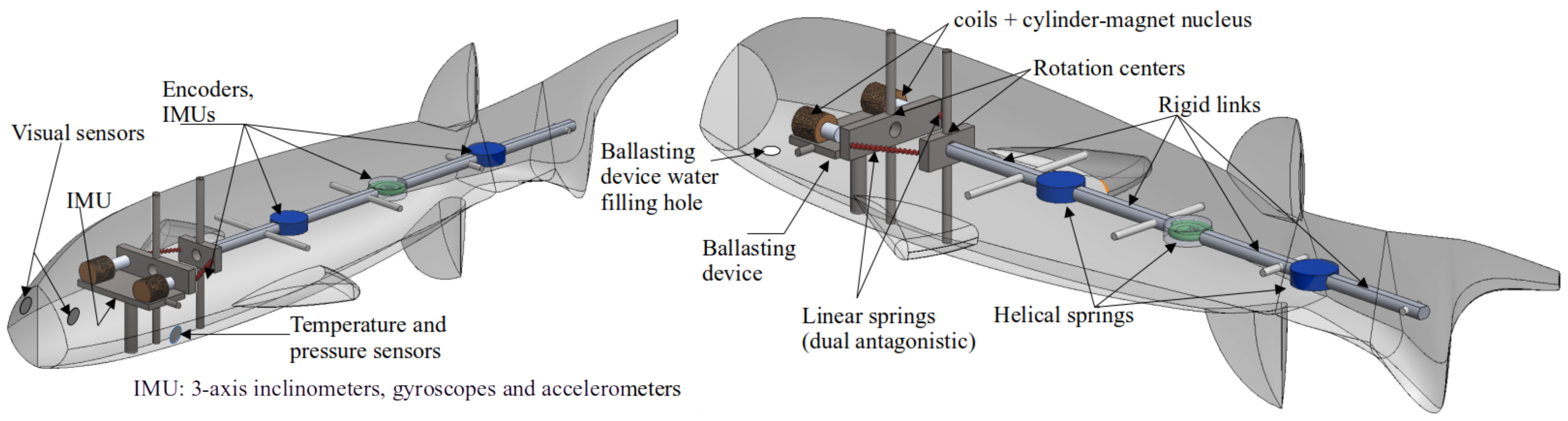
Figure 2 left provides an illustration of the geometric distribution of the sensing devices.
The instrumented robot is an embodiment of the human submerged in water, featuring an undulatory swimming mechanical body imbued with muscles possessing underactuated characteristics. These features empower the biorobotic avatar to execute movements and swim in its aquatic surroundings.
The observation models aim to provide insights into how these sensory perceptions are conveyed to the haptic helmet with haptic devices, including a wheel reaction mechanism. A comprehensive schema emerges wherein the haptic nexus, bolstered by pivotal human biosensorial components, including gravireceptors, Ruffini corpuscles, Paccinian receptors, and retinal photoreceptors, converges to interface with the sensory substrate of the human operator. Such a convergence engenders a cascading sequence wherein biological input stimuli coalesce to yield discernible encephalographic activity, the primary layer of subsequent electromyographic outputs. These consequential EMG outputs undergo processing in a swim oscillatory pattern generator, thereby embodying control of biomechanical cybernetic governance.
In accordance with
Figure 1, it is noteworthy that the various haptic input variables, such as temperature, pressure, and the visual camera images, represent direct sensory measurements transmitted from the robotic fish to the components of the haptic interface. Conversely, the robotic avatar takes on the role of a thermosensory adept in order for the human to assess the ambient thermal landscape. Thus, from this discernment, a surrogate thermal approach is projected onto the tactile realm of the human operator through the modulation of thermally responsive plates enmeshed within the haptic interface. Therefore, a crafted replica of the temperature patterns detected by the robotic aquatic entity is seamlessly integrated into the human sensory experience. This intertwining of thermal emulation is reached by the network of
Ruffini corpuscles, intricately nestled within the human skin, thereby enhancing the experiential authenticity of this multisensory convergence. As for interaction through the haptic functions, the
Paccinian corpuscles function as discerning receptors, proficiently registering subtle haptic pressures. It finds its origin in the dynamic tactile signals inherent to the aquatic habitat, intricately associated with the underwater depth traversed by the robotic avatar. Integral to the comprehensive sensory scheme, the optical sensors housed within the robotic entity acquire visual data. These visual data are subsequently channeled to the human’s cognition through the haptic interface’s perceptual canvas. Within this, the human sensory apparatus assumes the role of an engaged receptor, duly transducing these visual envoys through the lattice of retinal photoreceptors.
Embedded within the robotic fish’s body, several inertial measurement units (IMU) play a pivotal role in quantifying Eulerian inclinations intrinsic to the aquatic environment. These intricate angular displacements are subsequently channeled to the human operator, thereby initiating an engagement of the reaction wheel mechanism. As a consequential outcome of this interplay, a synchronized emulation of tilting motion is induced, mirroring the nuanced cranial adjustments executed by the human operator. Any alignment of movements assumes perceptible form, relayed through the human’s network of
gravireceptors nestled within the internal auditory apparatus. The Euler angular and linear speeds are not directly measured; instead, they must be integrated using various sensor fusion approaches to enhance the avatar’s fault tolerance in reading its environment. For example, the angular observations of the robot fish are obtained through numerical integro-differential equations, which are solved online as measurements are acquired. Let us introduce the following notation for inclinometers (
) and accelerometers (
), with the singular direct sensor measurement
derived from the gyroscopes. The observation for the fish’s roll velocity combining the three inertial sensors is
while the pitch velocity is modelled by
and the yaw velocity is obtained by
Within this context, the tangential accelerations experienced by the robot body are denoted [m/s2]. Additionally, the angular velocities measured by the gyroscopes are represented by [rad/s2]. Correspondingly, the inclinometers provide angle measurements denoted [rad]. These measurements collectively contribute to the comprehensive observability and characterization of the robot’s dynamic behavior and spatial orientation.
Furthermore, the oscillations of the caudal tail are reflections of the dynamics of the underactuated spine. These dynamics are captured by quantifying encoder pulses, denoted
, which provide precise angular positions for each vertebra. Given that real-time angular measurements of the vertebrae are desired, higher-order data are prioritized. Consequently, derivatives are computed by initiating from the Taylor series to approximate the angle of each vertebral element with respect to time, denoted
t.
thus, rearranging the math notation and trunking up to the first derivative,
dropping
off as a state variable, the first-order derivative (
) is given by
and assuming a vertebra’s angular measurement model in terms of the encoder’s pulses
with resolution
R, then it is stated that by substituting the pulses encoder model into the angular speed function for the first vertebra,
As for the second vertebra,
and
The preliminary sensing models serve as a comprehensive representation, strategically integrated into the control models as crucial feedback terms. A detailed exploration of this integration is elucidated in
Section 6 and
Section 7.
4. Deep ANN-Based EMG Data Classification
This section details the experimental acquisition of EMG data, their spatial filtering, and pattern extraction achieved through the statistical combination of linear envelopes. Additionally, an adaptive method for class separation and data dispersion reduction is described. This section also covers the structure of a deep neural network, presenting its classification output results from mapping input EMG stimuli.
A related study reported a system for automatic pattern generation for neurosimulation in [
34], where a neurointerface was used as a neuro-protocol for outputting finger deflection and nerve stimulation. In the present research, numerous experiments were carried out to pinpoint the optimal electrode placement and achieve precise electromyographic readings for each predefined movement in the experiment. The positions of the electrodes were systematically adjusted, and the results from each trial were compared. Upon data analysis, it was discerned that the most effective electrode placement is on the ulnar nerve, situated amidst the muscles flexor digitorium superficialis, flexor digitorium profundus, and flexor carpi ulnaris. A series of more than ten experiments was executed for each planned stimulus or action involving hands, allowing a 2s interval between each action, including the opening and closing of hands, as well as the extension and flexion of the thumb, index, middle, ring, and little fingers. The data were measured by a g.MOBIlab+ device with two-channel electrodes and quantified in microvolts per second [
v/s], as depicted in
Figure 3.
The data acquired from the electromyogram often exhibit substantial noise, attributed to both the inherent nature of the signal and external vibrational factors. To refine the data quality by mitigating this noise, a filtering process is essential.
In this context, a second-order Notch filter was utilized. This filter is tailored to target specific frequencies linked to noise, proving particularly effective in eliminating electrical interferences and other forms of stationary noise [
35]. A Notch filter is a band-rejection filter to greatly reduce interference caused by a specific frequency component or a narrow band signal. Hence, in the Laplace space, the second-order filter is represented by the analog Laplace domain transfer function:
where
signifies the cut angular frequency targeted for elimination, and
signifies the damping factor or filter quality, determining the bandwidth. Consequently, we solve to obtain its solution in the physical variable space. The bilinear transformation relates the variable
s from the Laplace domain to the variable
in the
domain, considering
T as the sampling period, and is defined as follows:
Upon substituting the previous expression into the transfer function of the analog Notch filter and algebraically simplifying, the following transfer function in the
domain is obtained, redefining the notation as
just to meet equivalence with the physical variable:
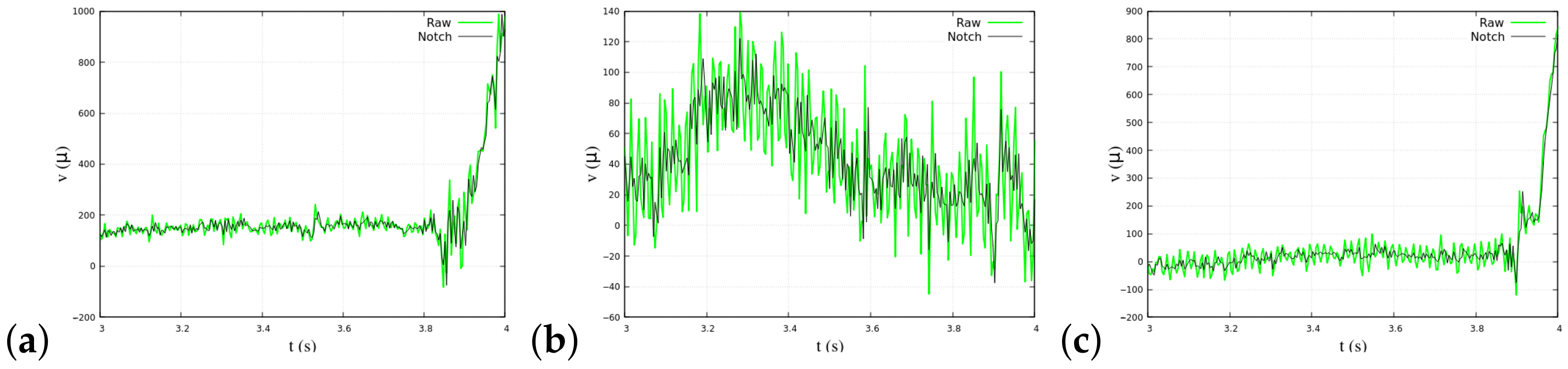
The second-order Notch filter
was employed on raw EMG data to alleviate noise resulting from electrical impedance and vibrational electrode interference, with parameters set at
Hz and
and results depicted in
Figure 4.
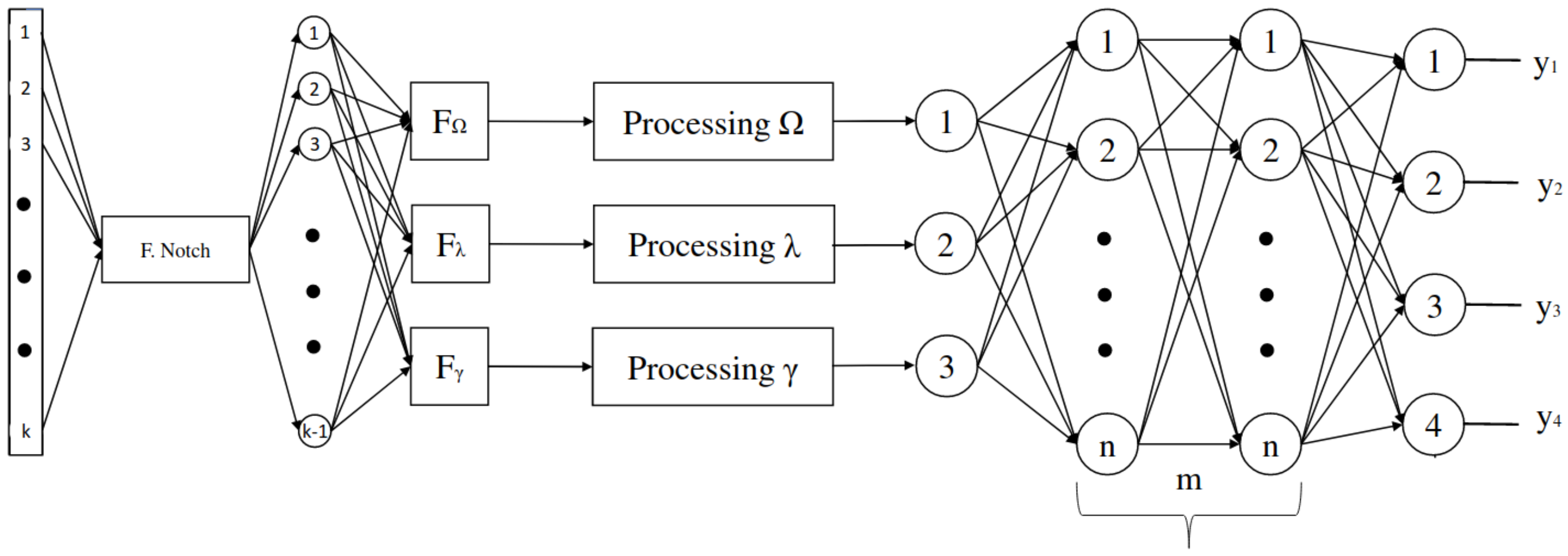
Subsequently, while other studies explored time and frequency feature extraction, as seen in [
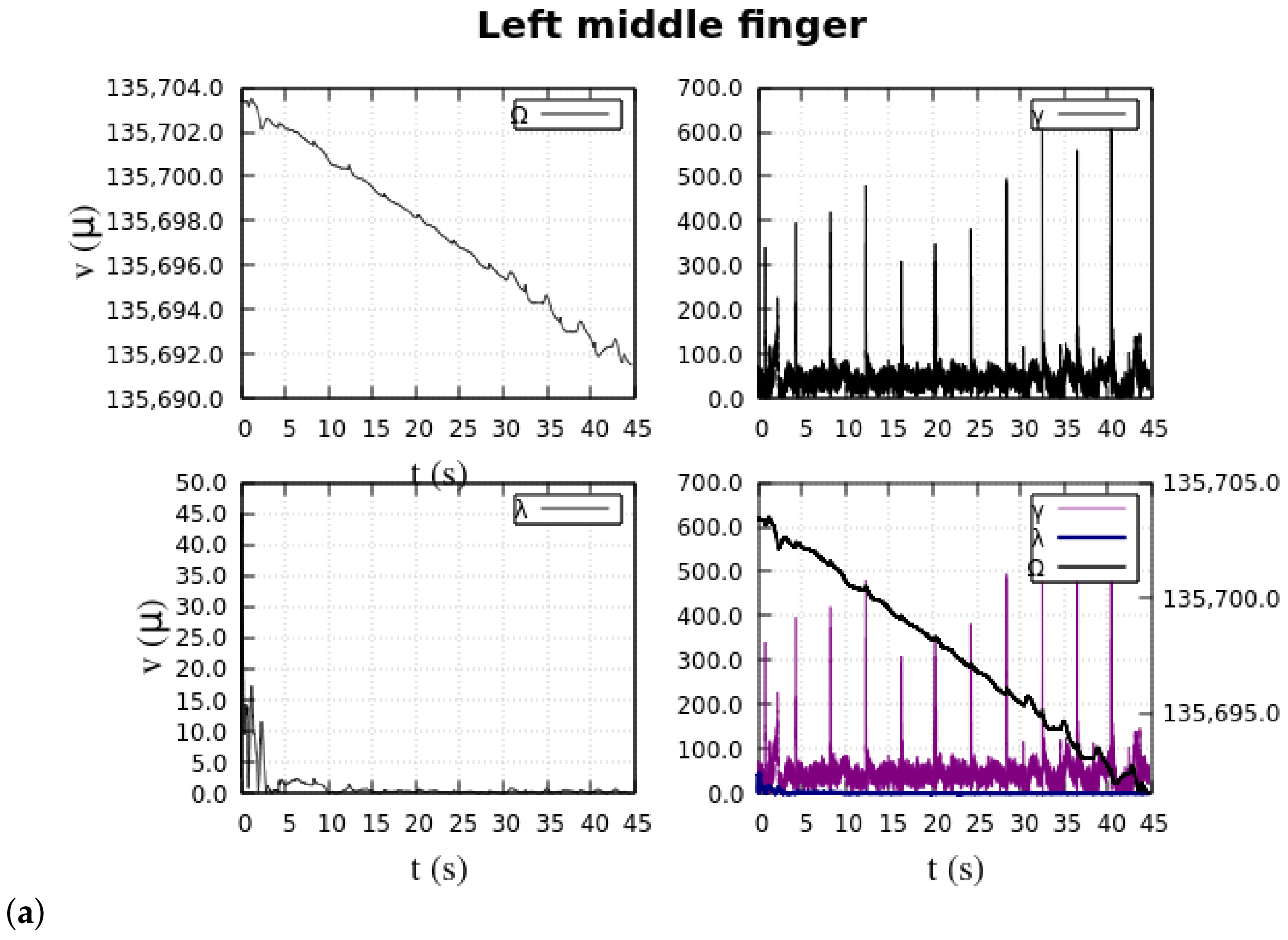
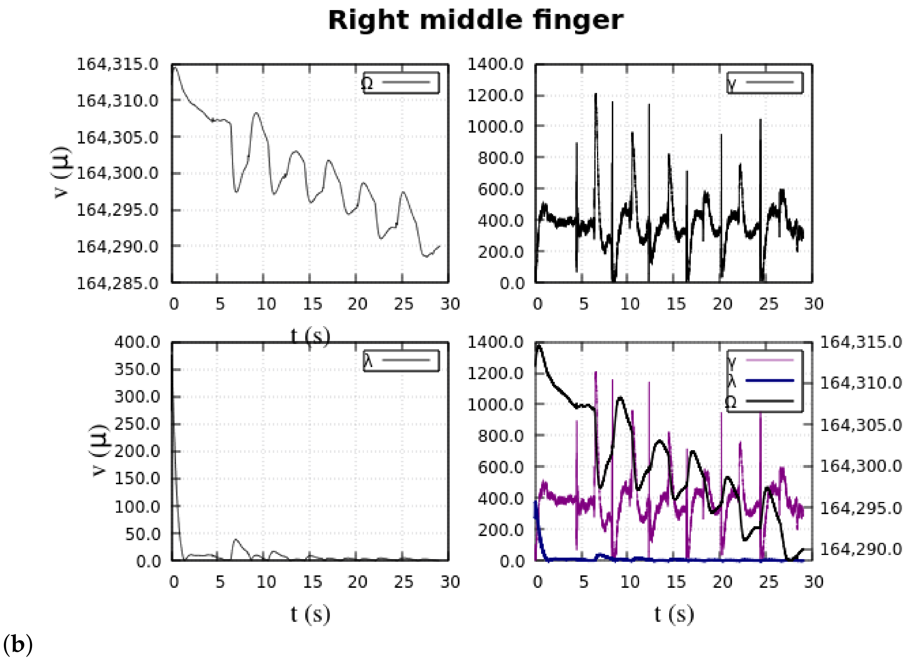
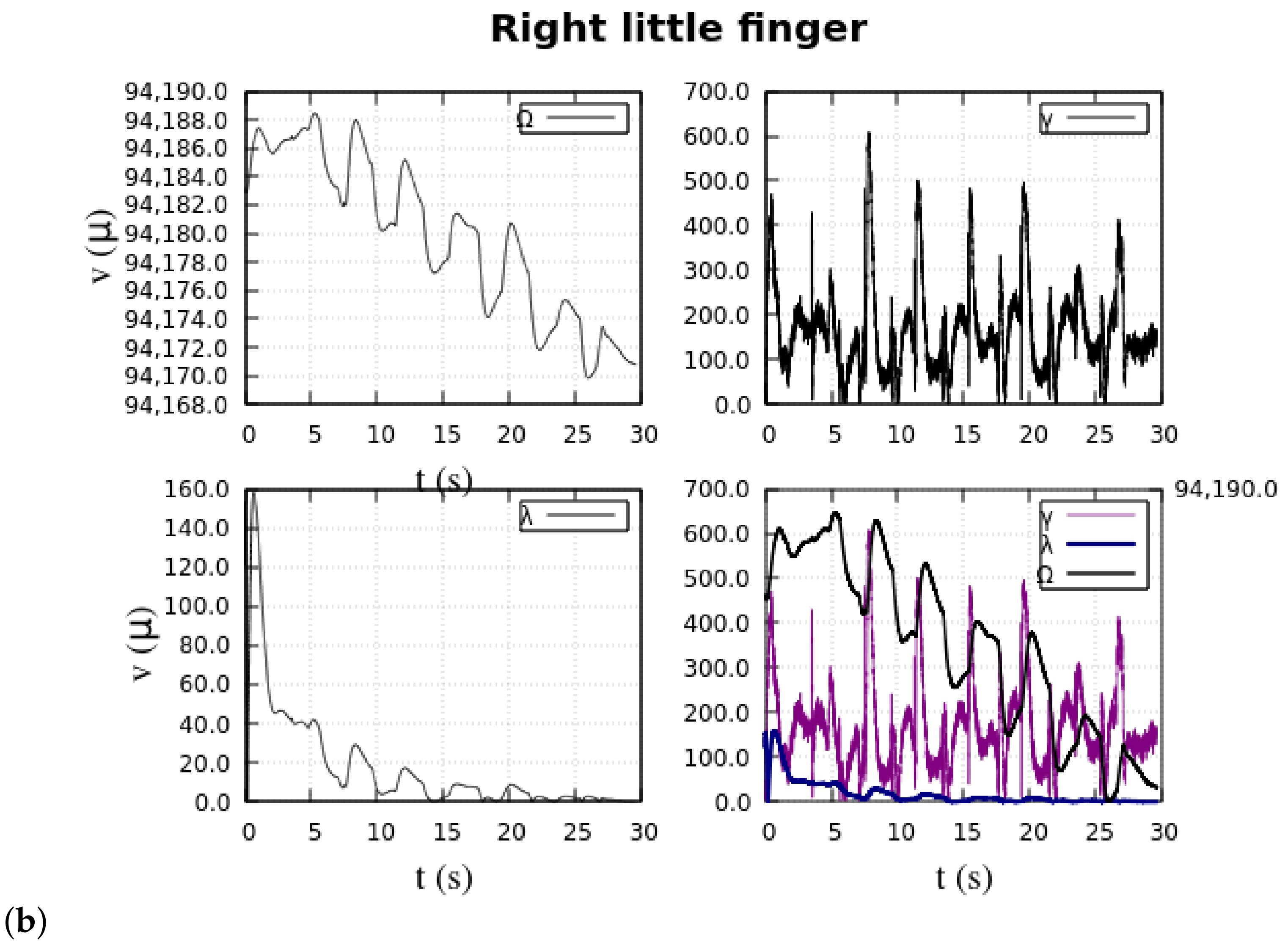
36], in the present context, by utilizing the outcomes of the Notch filter, our data undergo processing through three distinct filters or linear envelopes. This serves as a secondary spatial filter and functions as a pattern extraction mechanism. These include a filter for average variability, one for linear variability, and another for average dispersion. Each filter serves a specific purpose, enabling the analysis of different aspects of the signal. Consider
n as the number of measurements constituting a single experimental stimulus, and let
N represent the entire sampled data space obtained from multiple measurements related to the same stimulus. Furthermore, denote
as the
ith EMG measurement of an upper limb, measured in microvolts (
). From such statements, the following Propositions 1–3 are introduced as new data patterns.
Proposition 1 (Filter
).
The γ pattern refers to a statistical linear envelope described by the difference of a local mean in a window of samples and the statistical mean of all samples in an experiment. Proposition 2 (Filter
).
The pattern refers to a statistical linear envelope denoted by the difference of a local mean in a window of samples and the statistical mean of the whole population of experiments of the same type, Proposition 3 (Filter
).
The Ω
pattern refers to a statistical linear envelope denoted by the difference of statistical means between the population of one experiment and the whole population of numerous experiments of the same type: Hence, let the vector
such that
and represent filtered data points in the
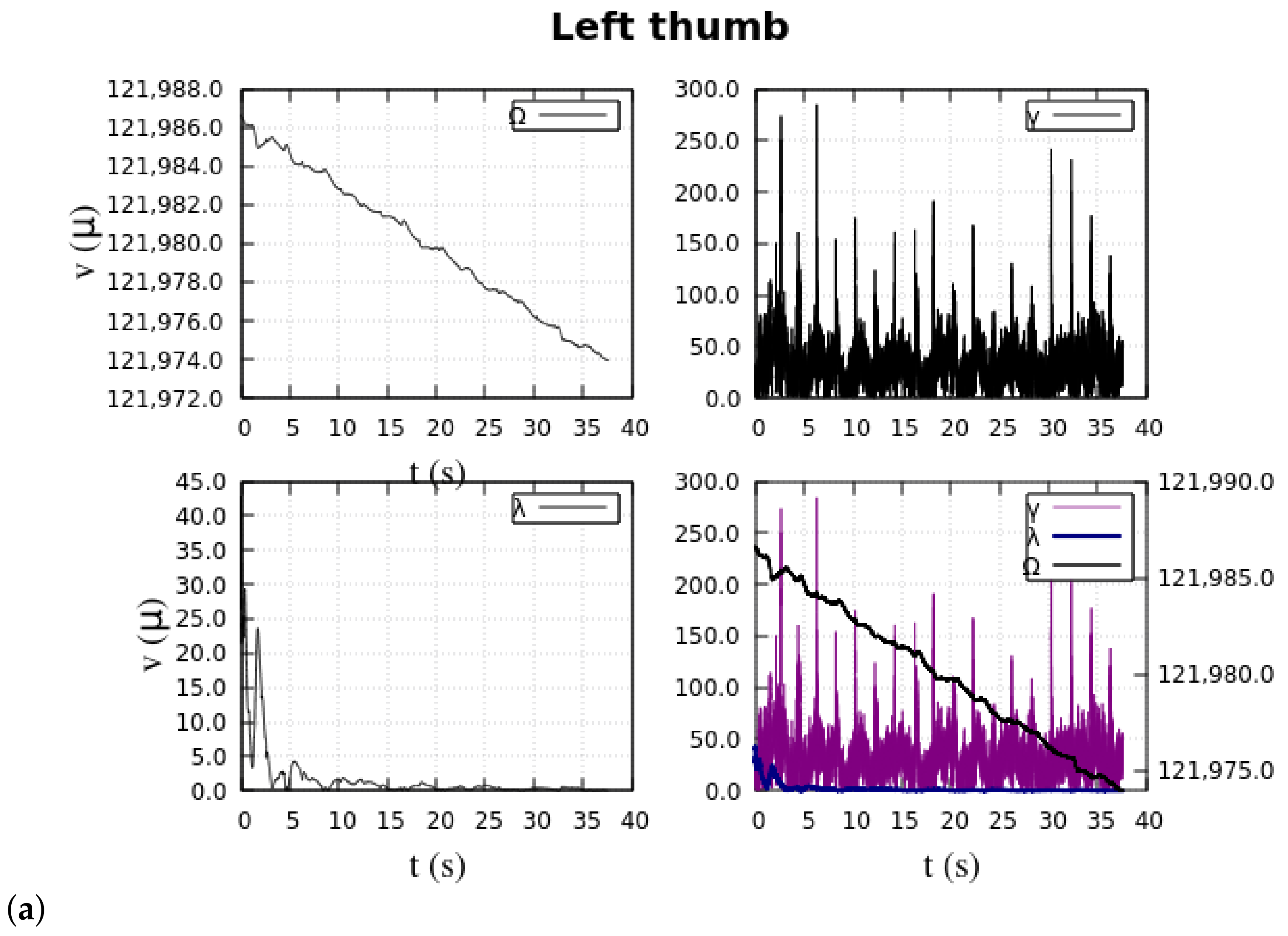
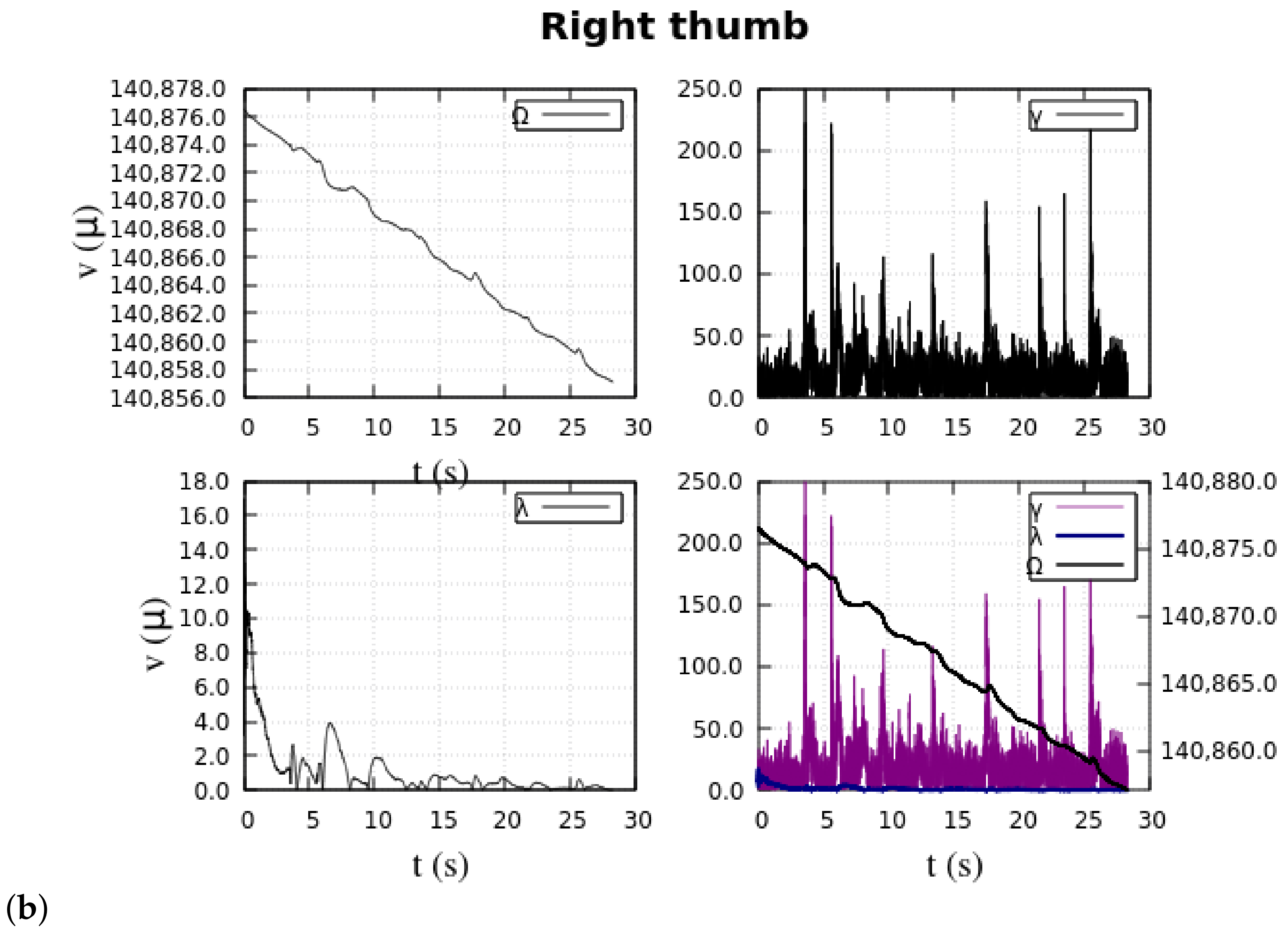
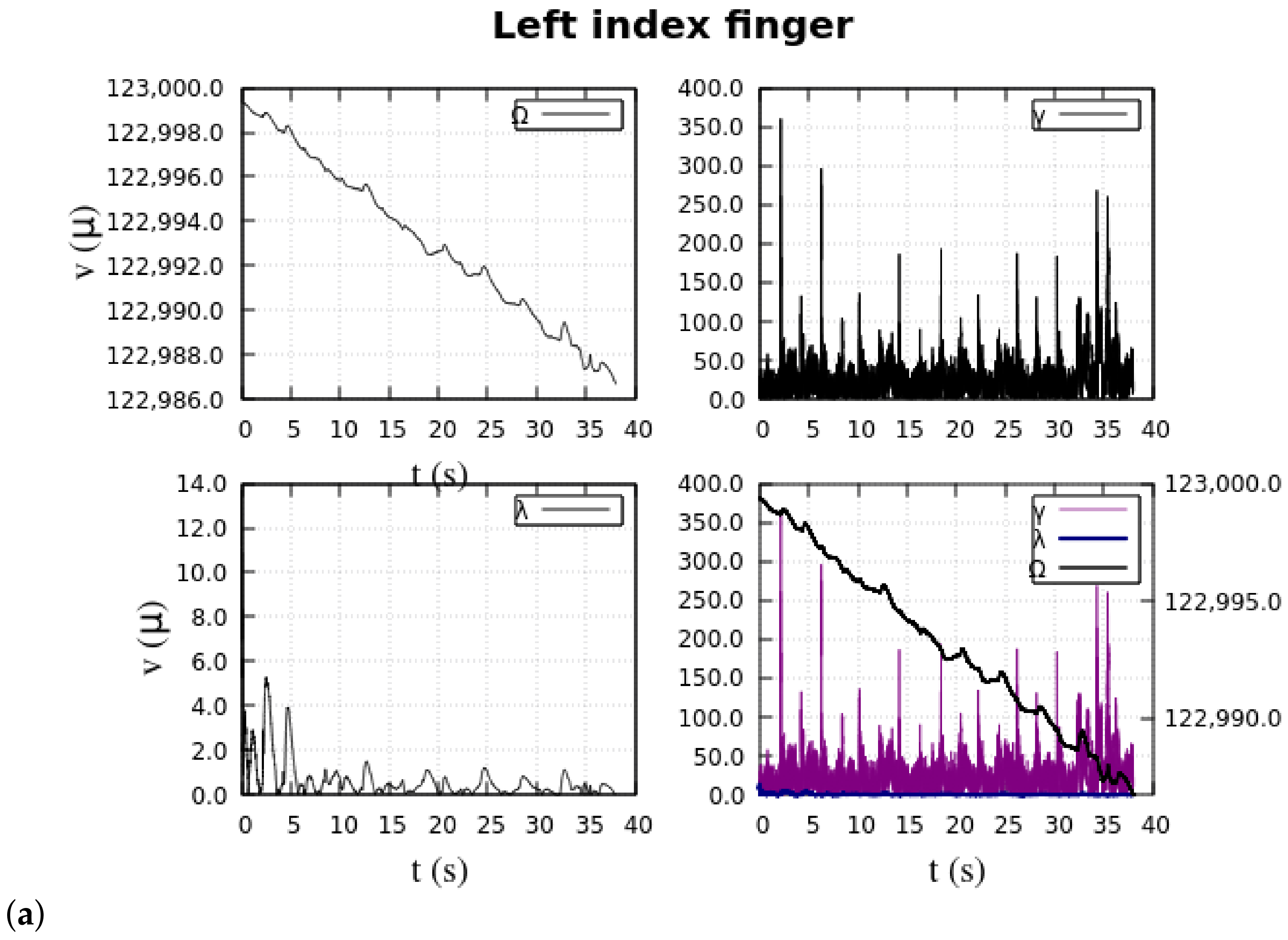
-space. This study includes a brief data preprocessing as a method to improve the multi-class separability and data scattering reduction in pattern extraction. Three distinctive patterns—
—captivatingly converge in
Figure 5. This illustration exclusively features patterns associated with sequences of muscular stimuli from both the right and left hands. For supplementary stimulus plots, refer to
Appendix A at the end of this manuscript.
From numerous laboratory experiments, over
of the sampled raw data fall within the range of one standard deviation. Consider the vector
such that the standard deviation vector
encompasses the three spatial components by its norm.
Building upon the preceding statement, we can formulate an adaptive discrimination criterion, as elucidated in Definition 1.
Definition 1 (Discrimination condition).
Consider the scalar value as preprocessed EMG data located within a radius of magnitude times the standard deviation :where represents discriminated data. Hence, consider the recent Definition 1 in the current scenario with
, which serves as a tuning discrimination factor. Therefore, the norm
represents the distance between the frame origin and any class in the
-space. This distance is adaptively calculated based on the statistics of each EMG class.
where the coefficients
,
, and
are smooth adjustment parameters to set separability along the axes. Hence, relocating each class center to a new position is stated by Proposition 4.
Proposition 4 (Class separability factor).
A new class position in the -space is established by the statistically adaptive linear relationship:andwhere are coarse in-space separability factors. The mean values are the actual class positions obtained from the linear envelopes , , and . Thus, by following the step-by-step method outlined earlier,
Figure 6 showcases the extracted features of the EMG data, representing diverse experimental muscular stimuli. These results hold notable significance in the research, as they successfully achieve the desired class separability and data scattering, serving as crucial inputs for the multilayer ANN.
Henceforth, the focus lies on identifying and interpreting the EMG patterns projected in the
-space, as illustrated in
Figure 6. The subsequent part of this section delves into the architecture and structure of the deep ANN employed as a classifier, providing a detailed account of the training process. Additionally, this section highlights the performance metrics and results achieved by the classifier, offering insights into its effectiveness. Despite the challenges posed by nonlinearity, multidimensionality, and extensive datasets, various neural network structures were configured and experimented with. These configurations involved exploring different combinations of hidden layers, neurons, and the number of outputs in the ANN.
A concise comparative analysis was performed among three distinct neural network architectures: the feedforward multilayer network, the convolutional network, and the competing self-organizing map. Despite notable configuration differences, efforts were made to maintain similar features, such as 100 training epochs, five hidden layers (except for the competing structure), and an equal number of input and output neurons (three input and four output neurons). The configuration parameters and results are presented in
Table 2. This study delves deeper into the feedforward multilayer ANN due to its superior classification rate. Further implementations with enhanced features are planned in the C/C++ language as a compiled program.
To achieve the highest success rate in accurate data classification through experimentation, the final ANN was designed with perceptron units, as depited in
Figure 7. It featured three inputs corresponding to the three EMG patterns
and included 12 hidden layers, each with 20 neurons. The supervised training process, conducted on a standard-capability computer, took approximately 20–30 min, resulting in nearly 1% error in pattern classification.
However, in the initial stages of the classification computations, with some mistuned adaptive parameters, the classification error was notably higher, even with much deeper ANN structures, such as 100 hidden layers with 99 neurons per layer. To facilitate the implementation, this work utilized the multilayer feedforward architecture increased to 300 epochs during training and implemented in C/C++, deploying the library Fast Artificial Neural Networks (FANN), generating extremely fast binary code once the ANN was trained. In the training process of this research, about 50 datasets from separate experiments for each type of muscular stimulus were collectively stored, each comprising several thousand muscular repetitions. A distinct classification label was assigned a priori for each class type within the pattern space. To demonstrate the reliability of the approach, 16 different stimuli per ANN were established for classification and recognition, resulting in the ANN having four combinatory outputs, each with two possible states.
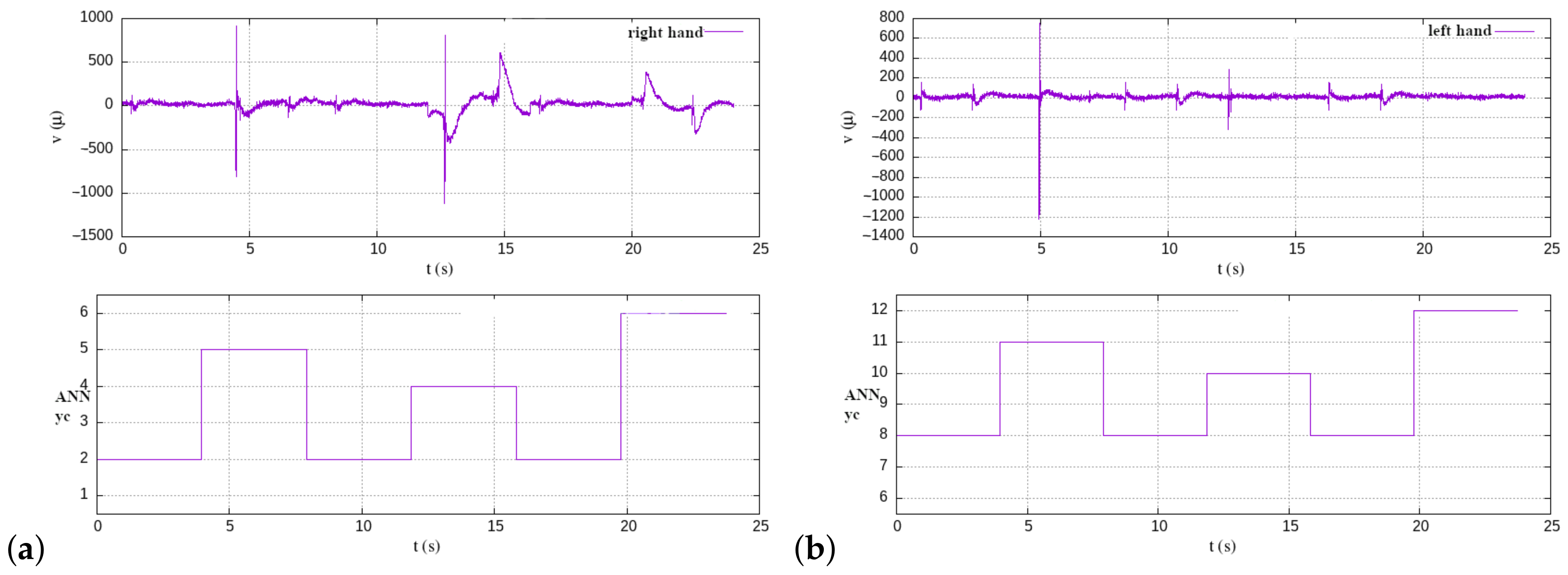
Figure 8 depicts mixed sequences encompassing all types of EMG stimuli, with the ANN achieving a 100% correct classification rate.
Moreover,
Table 3 delineates the mapping relationship between the ANN’s input, represented by the EMG stimuli, and the ANN’s output linked to a swimming behavior for controlling the robotic avatar.
5. Fuzzy-Based Oscillation Pattern Generator
This section delineates the methodology utilized to produce electric oscillatory signals, essential for stimulating the inputs of electromagnetic devices (solenoids) embedded within the mechanized oscillator of the biorobotic fish. The outlined approach for generating periodic electric signals encompasses three key components: (a) the implementation of a fuzzy controller; (b) the incorporation of a set of periodic functions dictating angular oscillations to achieve the desired behaviors in the caudal undulation of the fish; and (c) the integration of a transformation model capable of adapting caudal oscillation patterns into step signals, facilitating the operation of the dual-coil electromagnetic oscillator.
Another study [
37] reported a different approach, a neuro-fuzzy-topological biodynamical controller for muscular-like joint actuators. In the present research, an innovative strategy suggested for the fuzzy controller involves the combination of three distinct input fuzzy sets: the artificial neural network outputs transformed into crisp sets and the linear and angular velocities of the robot derived from sensor measurements. Simultaneously, the fuzzy outputs correspond to magnitudes representing the periods of time utilized to regulate the frequency and periodicity of the caudal oscillations. This comprehensive integration enables the fuzzy controller to effectively process both neural network-derived information and real-time sensor data, dynamically adjusting the temporal parameters that govern the fish’s undulatory motions.
The depiction of the outputs from the EMG pattern recognition neural network is outlined in
Table 3. Each binary output in the table is linked to its respective crisp-type input fuzzy sets when represented in the decimal numerical base
, as illustrated in
Figure 9a. Moreover, Definition 2 details the parametric nature of the input sets.
Definition 2 (Input fuzzy sets).
The output of the artificial neural network (ANN) corresponds to the fuzzy input, denoted , and only when it falls within the crisp set , the membership in the crisp set is referred to as .In relation to the sensor observations of the biorobot, the thrusting velocity v [cm/s] and angular velocity ω [rad/s] exhibit S-shaped sets modeled by sigmoid membership functions. This modeling approach is applied consistently to both types of input variables, capturing their extreme-sided characteristics. Let define the sets labeled “stop” and “fast” in relation to the thrusting velocity v, elucidated by Likewise, for the sets designated “left–fast” () and “right–fast” () concerning the angular velocity ω, the S-shaped sets are modeled as In addition, the rest of the sets in between are any of the kth Gauss membership functions (“slow”, “normal”, and “agile”) for the robot’s thrusting velocity with parametric mean and standard deviation ,and for its angular velocity (“left–slow”, “no turn”, and “right-slow”), with parametric mean and standard deviation , Therefore, the reasoning rules articulated in the inference engine have been devised by applying inputs derived from
Table 3, specifically tailored to generate desired outputs that align with the oscillation periods
T [s] of the fish’s undulation frequency (see
Figure 10).
Definition 3 (
).
For any linguistic value v representing sensor observations of the fish’s thrusting velocity,Likewise, for any linguistic value ω representing sensor observations of the fish’s angular velocity, Therefore, the following inference rules describe the essential robot fish swimming behavior.
if = sink and any or any then too_slow
if = buoyant and any or any then too_slow
if = gliding and any and any then slow, too_slow
if = slow_thrust and any and any then slow, too_slow
if = medium_thrust and any and any then normal, too_slow
if = fast_thrust and any and any then agile, too_slow
if = slow-right_maneuvering and any and any then too_slow, normal
if = medium-right_maneuvering and any and any then slow, agile, too_slow
if = fast-right_maneuvering and any and any then normal, fast, too_slow
if = slow-left_maneuvering and any and any then too_slow,
if = medium-left_maneuvering and any and any then slow, too_slow, agile
if = fast-left_maneuvering and any and any then normal, too_slow, fast
if = speed-up_right-turn and any and any then too_slow, fast
if = speed-up_left-turn and any and any then too_slow, fast
if = slow-down_right-turn and any and any then too_slow,
if y = slow-down_left-turn and any and any then too_slow, slow
Hence, the output fuzzy sets delineate the tail undulation speeds of the robot fish across the caudal oscillation period
T [s], as illustrated in
Figure 10. Notably, three identical output sets with distinct concurrent values correspond to the periods of three distinct periodic functions: forward (f), right (r), and left (l), as subsequently defined by Equations (
24a), (
24b), and (
24c).
The inference engine’s rules dictate the application of fuzzy operators to assess the terms involved in fuzzy decision-making. As for the thrusting velocity fuzzy sets, where
was previously established and by applying Definition 3, the fuzzy operator is described by
Likewise, the angular velocity fuzzy sets, where previously
was stated, by applying the second part of Definition 3, the following fuzzy operator is described by
Therefore, according to the premise (
or
), the following fuzzy operator applies:
Essentially, the fuzzification process applies strictly similar for the rest of the inference rules, according to the following Proposition.
Proposition 5 (Combined rules
).
The general fuzzy membership expression for the ith inference rule that combines multiple inference propositions isIn any crisp set, each attains a distinct value of 1, irrespective of the corresponding inference rule indexed by i. This value aligns with the ith entry in the neural network outputs outlined in Table 3. Additionally, k represents a specific fuzzy set associated with the same input. Executing the previously mentioned proposition, Remark 1 provides a demonstration of its application.
Remark 1 (Proposition 5 example).
Let us consider rule , where and either ( cm/s or rad/s). Thus, articulated in the context of the resulting fuzzy operator,Here, and . Based on the earlier proposition, the resulting , and given that rule 1 indicates an output period “too-slow”, its inverse outcome s. This outcome is entirely accurate, because the fish’s swim undulation will slow down up to 6 s, which is the slowest period oscillation.
Moving forward, during the defuzzification process, the primary objective is to attain an inverse solution. The three output categories for periods
T include “forward”, “right”, and “left”, all sharing identical output fuzzy sets of
T (
Figure 10). Nevertheless, the output fuzzy sets consist of two categories of distributions: Gauss and sigmoid distribution sets, as outlined in Definition 4. Regarding the Gauss distributions, their functional form is specified by:
Definition 4 (Output fuzzy sets).
The membership functions for both extreme-sided output sets are defined as “fast” with and “too slow” with , such thatHere, T [s] denotes the period of time for oscillatory functions, with the slope direction determined by its sign. The parameter c represents an offset, and k is the numerical index of a specific set.
Furthermore, the membership functions for three intermediate output sets are defined as “agile” with , “normal” with , and “slow” with , such that: Here, represents the mean value, and denotes the standard deviation of set k, with k serving as the numeric index of a specific set.
In accordance with Definition 4, any
possesses a normalized membership outcome within the interval
. The inverse sigmoid membership function, denoted
∀
, is determined by the general inverse expression:
Similarly, the inverse Gaussian membership function, where
∀
, is defined by the inverse function:
Hence, exclusively for the
jth category among the output fuzzy sets affected by the fuzzy inference rule essential for estimating the value of
T, the centroid method is employed for defuzzification through the following expression:
or more specifically,
For terms
and
, the inverse membership function (
20) is applicable, whereas for the remaining sets in the
jth category, the inverse membership (
21) is applied.
Reference [
38] reported a CPG model to control a robot fish’s motion in swimming and crawling and let it perform different motions influenced by sensory input from light, water, and touch sensors. The study of [
39] reported a CPG controller with proprioceptive sensory feedback for an underactuated robot fish. Oscillators and central pattern generators (CPGs) are closely related concepts. Oscillators are mathematical or physical systems exhibiting periodic behavior and are characterized by the oscillation around a stable equilibrium point (limit cycle). In the context of CPGs, these are neural networks that utilize oscillators that create positive and negative feedback loops, allowing for self-sustaining oscillations and the generation of rhythmic patterns, particularly implemented in numerous robotic systems [
40]. CPGs are neural networks found in the central nervous system of animals (e.g., fish swimming [
41]) that generate rhythmic patterns of motor activity and are responsible for generating and coordinating optimized [
42] repetitive movements.
The present research proposes a different approach from the basic CPG model, and as a difference from other wire-driven robot fish motion approaches [
43], this study introduces three fundamental undulation functions: forward, right-turning, and left-turning. These functions are derived from empirical measurements of the robot’s caudal fin oscillation angles. However, a distinctive behavioral undulation swim is achieved by blending these three oscillation functions, each incorporating corresponding estimation magnitudes derived from the fuzzy controller outputs. The formulation of each function involves fitting empirical data through Fourier series. As a difference from other approaches on CPG parameter adjustment [
44], the preceding fuzzy outputs obtained from (
23) to estimate time periods
play a pivotal role in parameterizing the time periods for the periodic oscillation functions, as outlined in Proposition 6.
Proposition 6 (Oscillation pattern function). Three fundamental caudal oscillation patterns, designed to generate swimming undulations, are introduced, each characterized by 11 pre-defined numerical coefficients. These patterns are described by amplitude functions, denoted , where ϕ represents oscillation angles, and the time period T is an adjustable parameter.
The undulation pattern for forward motion is provided by the following function: Likewise, the undulation pattern for right-turn motion is given by the function Finally, the undulation pattern for left-sided turning motion is established by the expression The approaches to forward, right-turn, and left-turn based on the findings of Proposition 6 are illustrated in
Figure 11. Additionally, a novel combined oscillation pattern emerges by blending these three patterns (
25), each assigned distinct numerical weights through the neuro-fuzzy controller.
The proposed robotic mechanism features a multilink-based propulsive spine driven by an electromagnetic oscillator composed of a pair of antagonistic solenoids that necessitate a synchronized sequence of electric pulses (see
Figure 12b). The amplitudes generated by
in Equation (
25) essentially represent the desired undulation pattern for the robotic fish’s caudal fin. However, these oscillations are not directly suitable for the inputs of the coils. To address this, our work introduces a decomposition of
into two step signals centered around a stable equilibrium point (limit cycle), one for the right coil (positive with respect to the limit cycle) and another for the left coil (negative with respect to the limit cycle). The coil’s step function, for either the right-sided or left-sided coil, is given by
, taking the equilibrium point as their limit value
:
The Boolean
values derived from (
26) are illustrated in
Figure 11a–c as sequences of step signals for both the right (R) and left (L) solenoids of the robot. Each plot maintains a uniform time scale, ensuring vertical alignment for clarity. In contrast to the work presented in [
45] focusing on the swimming modes and gait transition of a robotic fish, the current study, as depicted in
Figure 11, introduces a distinctive context. The three oscillatory functions,
, are displayed both overlapped and separated, highlighting their unique decoupled step signals. Assuming
for all
in each case, in
Figure 11a,
, with
; in
Figure 11b,
, with
; and in
Figure 11c,
, with
. For a more comprehensive understanding,
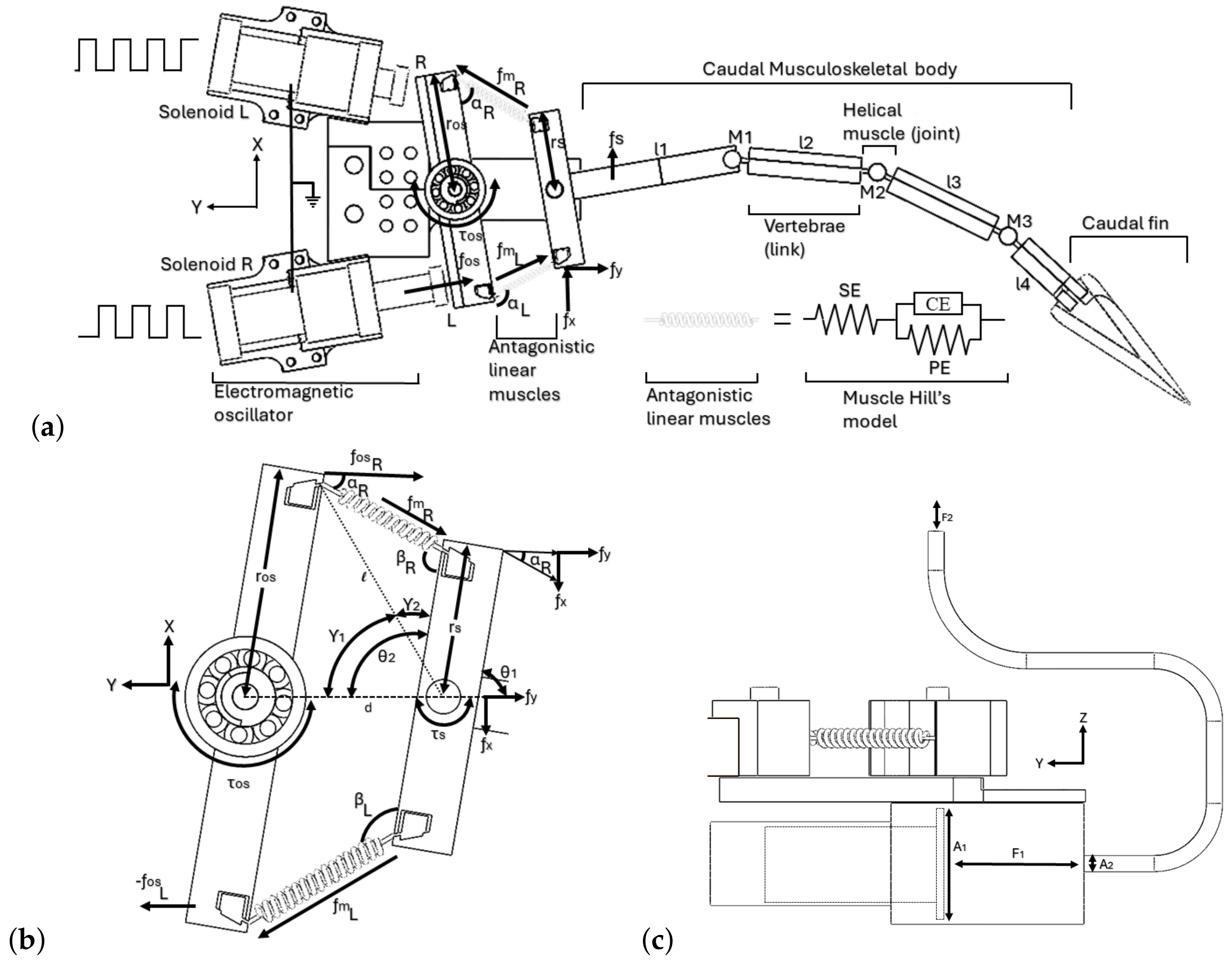
Figure 12b presents the electromechanical components of the caudal motion oscillator.
6. Robot Fish Biomechanical Model
This section introduces the design of the robotic fish mechanism and explores the model of the underactuated physical system to illustrate the fish undulation motions. The conceptualization of the proposed system is inspired by an underactuated structure featuring a links-based caudal spine with passive joints, utilizing helical springs to facilitate undulatory locomotion (see
Figure 12a). The robotic fish structure introduces a mechanical oscillator comprising a pair of solenoids activated through coordinated sequences of step signals, as described by (
26). Essentially, the electromagnetic coils generate antagonistic attraction/repulsion linear motions, translating into rhythmic oscillations within a mechanized four-bar linkage (depicted in
Figure 12b). This linkage takes on the form of a trapezoid composed of two parallel rigid links and two lateral linear springs functioning as antagonistic artificial muscles. Moreover, beneath the electromagnetic oscillator, there is a ballasting device for either submersion or buoyancy (
Figure 12c). The robot’s fixed reference system consists of the
X axis, which intersects the lateral sides, and the
Y axis aligned with the robot’s longitudinal axis.
In
Figure 12a, the electromagnetic oscillator of the robotic avatar responds to opposing coordinated sequences of step signals. The right-sided (R) and left-sided (L) solenoids counteract each other’s oscillations, generating angular moments in the trapezoid linkage (first vertebra). Both solenoids are identical, each comprising a coil and a cylindrical neodymium magnet nucleus. The trapezoid linkage, depicted in
Figure 12b, experiences magnetic forces
at the two neodymium magnet attachments situated at a radius of
, resulting in two torques,
and
, with respect to their respective rotation centers. As input forces
come into play, the linear muscle in its elongated state stores energy. Upon restitution contraction, this stored energy propels the rotation of the link
, which constitutes the first vertebra of the fish.
Furthermore, the caudal musculoskeletal structure, comprising four links () and three passive joints (), facilitates a sequential rotary motion transmitted from link 1 to link 4. This transmission is accompanied by an incremental storage of energy in each helical spring that is serially connected. Consequently, the last link (link 4) undulates with significantly greater mechanical advantage. In summary, a single electrical pulse in any coil is sufficient to induce a pronounced undulation in the swimming motion of the robot’s skeleton.
As for the ballasting control device situated beneath the floor of the electromechanical oscillator, activation occurs only when either of two possible outputs from the artificial neural network (ANN) is detected: when equals “sink” or “buoyancy”. However, the fuzzy nature of these inputs results in a gradual slowing down of the fish’s undulation to its minimum speed. Additionally, both actions are independently regulated by a dedicated feedback controller overseeing the ballasting device.
Now, assuming knowledge of the input train of electrical step signals
applied to the coils, let us derive the dynamic model of the biorobot, starting from the electromagnetic oscillator and extending to the motion transmitted to the last caudal link. Thus, as illustrated in
Figure 12a,b, the force
f [N] of the solenoid’s magnetic field oscillator is established on either side (right, denoted R, or left, denoted L),
In this context,
A [m
2] represents the area of the solenoid’s pole. The symbol
denotes the magnetic permeability of air, expressed as
H/m (henries per meter). Hence, the magnetic field
B (measured in Teslas) at one extreme of a solenoid is approximated by:
where
i represents the coil current [A],
N is the number of wire turns in a coil, and
l denotes the coil length [m]. Furthermore, a coil’s current is described by the following linear differential equation as a function of time
t (in seconds), taking into account a potential difference
(in volts):
Here,
L represents the coil’s inductance (measured in henries, H) with an initial current condition denoted
. Additionally, the coil’s induction model is formulated by:
In essence, this study states that both lateral solenoids exhibit linear motion characterized by an oscillator force
. This force is expressed as:
and due to the linear impacts of solenoids on both sides R and L (refer to
Figure 12a), the first bar of the oscillator mechanism generates a torque, expressed as:
It is theorized that the restitution/elongation force along the muscle is denoted
(R or L), with this force being transmitted from the electromechanical oscillator to the antagonistic muscle in the opposite direction (refer to
Figure 12b). This implies that the force generated from the linear motion solenoid in the oscillator’s right-sided coil, denoted
, is applied at point R and subsequently reflected towards point L with an opposite direction, represented as
. Similarly, conversely from the oscillator’s left-sided solenoid, the force
is applied at point L and transmitted to point R as
. For
applied in L,
Hence, the angles
assume significance as the forces acting along the muscles
differ, resulting in distinct instant elongations
. Consequently, the four-bar trapezoid-shaped oscillator mechanism manifests diverse inner angles, namely,
,
, and
, as illustrated in
Figure 12b.
Thus, prior to deriving an analytical solution for
, it is imperative to formulate a theoretical model for the muscle. In this study, a Hill’s model is adopted, as depicted in
Figure 12a (on the right side). The model incorporates a serial element SE (overdamped), a contractile element CE (critically damped), and a parallel element PE (critically damped), each representing distinct spring-mass-damper systems.
The generalized model for the antagonistic muscle is conceptualized in terms of the restitution force, and it is expressed as:
Therefore, by postulating an equivalent restitution/elongation mass
associated with instantaneous weight-force loads
w (such as due to hydrodynamic flows), the preceding model is replaced with Newton’s second law of motion,
Furthermore, through the independent solution of each element within the system in terms of elongations, the SE model can be expressed as:
Here,
represent arbitrary constants representing the damping amplitude. The terms
denote the root factors,
Here, the factors are expressed in relation to the damping coefficient (in kg/s) and the elasticity coefficient (in kg/s2).
Similarly, for the contractile element CE, its elongation is determined by:
With amplitude factors
and damping coefficient
a similar expression is obtained for the parallel element PE:
With amplitude factors
and damping coefficient
the next step involves substituting these functional forms into the general muscle model,
such that the complete muscle’s force model
is formulated by
Subsequently, simplifying the preceding expression leads to the formulation presented in Proposition 7.
Proposition 7 (Muscle force model).
The solution to the muscle force model, based on a Hill’s approach, is derived as a time-dependent function encompassing its three constituent elements (serial, contractile, and parallel). This formulation is expressed as: Thus, without loss of generality, considering a muscle model characterized by elongation and a force-based model , we proceed to derive the passive angles of the oscillator and the output forces and for .
Under initial conditions, the trapezoid oscillator bars are assumed to have
, aligning the four-bar mechanism with the
X axis. As the bars rotate by an angle
due to solenoid impacts at points R or L, the input bar of the oscillator with a radius of
undergoes an arc displacement
. Simultaneously, the output bar of shorter radius
experiences a displacement rate of
, such that:
The arc displacement at point R or L is given by
. Consequently, the rotation angle of the input oscillator is expressed as:
Therefore, by formulating this relationship in the context of forces and subsequently substituting the newly introduced functions, the resulting expression is
Here,
denotes the linear acceleration of either point R or L along the robot’s
Y axis. By replacing the solenoid’s mass-force formulation,
Hence, the functional expression for
takes the form
Without loss of generality, the inner angle
of the oscillator mechanism (refer to
Figure 12b) is derived as:
Initially, when the oscillator bars are aligned with respect to the
X axis, an angular displacement denoted by
occurs as a result of the transfer of motion from the solenoid’s tangential linear motion to the input bar. Similarly, in the output bar, the corresponding angular displacement is represented by
,
Here,
signifies a minute variation resulting from motion perturbation along the various links of the caudal spine. The selection of the ± operator depends on the robot’s side, whether it is denoted R or L. As part of the analysis strategy, the four-bar oscillator was geometrically simplified to half a trapezoid for the purpose of streamlining deductions (refer to
Figure 12b). Within this reduced mechanism, two triangles emerge. One triangle is defined by the parameters
,
ℓ,
d, while the other is characterized by
, where
ℓ serves as the hypotenuse and the sides
d,
, and
remain constant. Consequently, the instantaneous length of the hypotenuse is deduced as follows:
Upon determining the value of
ℓ, the inner angle
can be derived as follows:
Therefore, by isolating
,
Until this point, given the knowledge of
and
, it is feasible to determine the inner complementary angle
through the following process:
Subsequently, the angle formed by the artificial muscle and the output bar can be established according to the following principle:
Thus, the inner angle
is
or, alternatively, an approximation of the muscle length is
This is the mechanism through which the input bar transmits a force
, as defined in expression (
33), from the tangent
to the output bar, achieving a mechanical advantage denoted
,
Hence, in accordance with the earlier stipulation in expression (
33), Definition 5 delineates the instantaneous angles
.
Definition 5 (Angles
).
The instantaneous angle α, expressed as a function of the inner angles of the oscillator, is introduced by: It is noteworthy that, owing to the inertial system of the robot, the longitudinal force output component
aligns with the input force
in direction. Consequently, for a right-sided force, we have
, where:
and
Likewise, for the left-sided
,
as well as
In this scenario, an inverse solution is only applicable for
, with no necessity for determining
. Consequently, the mechanical advantage transferred between the input and output bars can be expressed by a simplified coefficient
Furthermore, through the utilization of the following trigonometric identity,
can substitute and streamline the ensuing system of nonlinear equations by solving them simultaneously. Additionally, let
be defined as:
Hence, the simultaneous nonlinear system is explicitly presented solely for the force components along the
X axis:
and
Therefore, for the numerical solution of the system, a multidimensional Newton–Raphson approach is employed as outlined in the provided solution:
and
Thus, by defining all derivative terms to finalize the system,
Therefore, by subsequently organizing and algebraically simplifying,
and
The objective is to achieve numerical proximity, aiming for
. Consequently, through this inverse solution, the lateral force components of the first spinal link, denoted by
, are intended to be estimated because they are perpendicular to the links and produce the angular moments at each passive joint.
Thus, given that the torque of the trapezoid’s second bar is
(see
Figure 12b), we establish a torque–angular moment equivalence, denoted
. Leveraging this equivalence and the prior understanding of the torque
acting on the second bar of the trapezoid, mechanically connected to the first link
, we affirm their shared angular moment. Consequently, the general expression for the tangential force
applied at the end of each link
is:
Yet, considering the angular moment
for each helical-spring joint, supporting the mass of the successive links, let us introduce equivalent inertial moments, starting with
. Subsequently, we define
,
, and finally,
. Thus, in the continuum of the caudal spine, the transmission of energy to each link is contingent upon the preceding joints, as established by
Each helical spring, connecting pairs of vertebrae, undergoes an input force
, directly proportional to the angular spring deformation indicated by elongation
x. Here,
k [kg m
2/s
2] represents the stiffness coefficient. External forces result in an angular moment, given by
, where torque serves as an equivalent variable to angular momentum, such that
. Consequently, when expressing the formula as a linear second-order differential equation, we have:
Here,
represents undulatory accelerations arising from external loads or residual motions along the successive caudal links, which are detectable through encoders and IMUs. Assuming an angular frequency
, a period
, and moments of inertia expressed as
, the general equation is formulated as follows:
where
is replaced by the helical spring expression (
71) to derive
By algebraically extending, omitting terms, and rearranging for all links in the caudal spine, we arrive at the following matrix-form equation:
Hence, in accordance with Expression (
69), the tangential forces exerted on all the caudal links of the robotic fish are delineated by the following expression:
Alternatively, the last expression can be denoted as the following control law:
where
,
represents mass dispersion, and
denotes the vector of angular accelerations for the caudal vertebrae, including external loads. Additionally,
stands for the matrix of stiffness coefficients. Therefore, the inverse dynamics control law, presented in a recursive form, is:
Finally, for feedback control, both equations are simultaneously employed within a computational recursive scheme, and angular observations are frequently derived from sensors on both joints: encoders and IMUs.
7. Ballasting Control System
This section delineates the integration of the ballasting control system, crafted to complement the primary structure of the biorobot. It introduces the ballasting model-based control system, selectively activated in response to the artificial neural network’s (ANN) output, particularly triggered when the ANN signals “sink” or “buoyancy”.
Figure 13a visually depicts the biorobot’s ballasting system, while
Figure 13b presents a diagram illustrating the fundamental components of the hydraulic piston, crucial for control modeling.
The core operational functions of the ballasting device involve either filling its container chamber with water to achieve submergence or expelling water from the container to attain buoyancy. Both actions entail the application of a linear force for manipulating a plunger or hydraulic cylindrical piston, thereby controlling water flow through either suction or exertion. Consequently, the volume of the liquid mass fluctuates over time, contingent upon a control reference or desired level marked H, along with quantifying a filling rate and measuring the actual liquid level .
Hence, we can characterize the filling rate
as the change in volume
V with respect to time, expressed as
and assuming a cylindrical plunger chamber with radius
r and area
, the volume is expressed as
Here,
represents the actual position of the plunger due to the incoming hydraulic mass volume. Consequently, the filling rate can also be expressed as
Consider
k as an adjustment coefficient, and let
H be the reference or desired filling level. The instantaneous longitudinal filling level is denoted
. By substituting the previous expressions into the initial Equation (
78), we derive the following first-order linear differential equation:
To solve the aforementioned equation, we employ the integrating factor method, such that
In this instance, the integrating factor is determined as follows:
Thus, by applying the integrating factor, we effectively reduce the order of derivatives in the subsequent steps,
Through algebraic simplification of the left side of the aforementioned expression, the following result is determined:
Following this, by integrating both sides of the equation with respect to time,
where the expression on the left side undergoes a transformation into
and the right side of the equation, once solved, transforms into
Now, to obtain the solution for
, it is isolated by rearranging the term
:
For initial conditions where
indicates the plunger is completely inside the contained chamber at the initial time
s, the integration constant
c is determined as
Therefore, the value of
c takes on
, and substituting it into the previously obtained solution,
In addition, considering that the required force of the piston
is hence given by:
where
is the friction force of the piston in the cylindrical piston, and
refers to the water pressure at that depth over the piston’s entry area. The instantaneous mass considers the piston’s mass
and the liquid mass of the incoming water
:
where the water density is
and
, thus completing the mass model:
Therefore, the force required to pull/push the plunge device is stated by the control law, given as
Finally, two sensory aspects were considered for feedback in the ballast system control and depth estimation. Firstly, the ballast piston is displaced by a worm screw with an advance parameter
[m] and a motor, whose sensory measurement is taken at motor rotations
by a pulses
encoder of angular resolution
R, where
. This allows for the instantaneous position of the piston to be measured by the observation
,
Secondly, the robot’s aquatic depth estimation, denoted as
, is acquired using a pressure sensor as previously described in
Figure 2. This involves measuring the variation in pressure according to Pascal’s principle between two consecutive measurements taken at different times.
where the instantaneous fluid force at a certain depth is expressed in terms of the measured pressure
. Additionally, the area of the fish body subjected to fluid force
, and robot of mass
and averaged area
,
Assuming an ideal fluid, and substituting the fluid forces in terms of measurable pressures, as well as expressing the fish mass in terms of its density
and volume
, which describes the weight of the robot’s body. It follows
where
and
represent the surface depth and the actual depth of the robot, respectively, such that
denotes the total depth. Therefore,
and by determining the pressure in the liquid as a function of depth, we select the level of the liquid’s free surface such that
, where
represents the atmospheric pressure, resulting in
Establishing
as the water pressure sensor measurement. Thus, the feedback robot fish depth estimation is given by
8. Conclusions and Future Work
In summary, this study introduces a cybernetic control approach integrating electromyography, haptic feedback, and an underactuated biorobotic fish avatar. Human operators control the fish avatar using their muscular stimuli, eliminating the need for handheld apparatus. The incorporation of fuzzy control, combining EMG stimuli with motion sensor observations, has proven highly versatile in influencing the decision-making process governing the fish’s swimming behavior. The implementation of a deep neural network achieved remarkable accuracy, surpassing , in recognizing sixteen distinct electromyographic gestures. This underscores the system’s robustness, effectively translating human intentions into precise control commands for the underactuated robotic fish.
The adoption of robotic fish technologies as human avatars in deep-sea exploration offers significant benefits and implications. Robotic fish avatars enable more extensive and efficient exploration of hazardous or inaccessible deep-sea environments, leading to groundbreaking discoveries in marine biology, geology, and other fields. By replacing human divers, robotic avatars mitigate risks associated with deep-sea exploration, ensuring the safety of researchers by avoiding decompression sickness, extreme pressure, and physical danger. Robotic avatar technology presents a more cost-effective alternative to manned missions, eliminating the need for specialized life support systems, extensive training, and logistical support for human divers. Robotic avatars facilitate continuous monitoring of deep-sea ecosystems, collecting data over extended periods without being limited by human endurance or logistical constraints. Minimizing human presence in the deep sea reduces environmental disturbance and the risk of contamination or damage to fragile ecosystems, preserving them for future study and conservation efforts. The development of robotic fish technologies drives innovation in robotics, artificial intelligence, and sensor technologies, with potential applications extending beyond marine science into various industries. Overall, while robotic fish avatars offer numerous benefits for deep-sea exploration and research, their deployment should be carefully managed to maximize scientific advancement while minimizing potential negative consequences.
While the adoption of robotic fish avatars holds significant promise for deep-sea exploration, several limitations and areas for future research must be addressed. Developing robotic fish avatars capable of accurately mimicking the behaviors of real fish in diverse deep-sea conditions remains a considerable challenge, necessitating improvements in propulsion, maneuverability, and energy efficiency. Enhancing their sensory capabilities to detect environmental stimuli effectively, alongside improving communication systems for real-time data transmission, is crucial for efficient exploration and navigation. Additionally, these avatars must adapt to the harsh deep-sea conditions, requiring research into materials and components that withstand extreme pressures, low temperatures, and limited visibility while maintaining functionality. Ensuring their long-term reliability and durability through maintenance strategies and robust designs is essential for sustained exploration missions. Integrating robotic fish avatars with emerging technologies like artificial intelligence and advanced sensors could further enhance their effectiveness. Addressing these challenges through continued research is vital for realizing the full potential of robotic fish avatars in deep-sea exploration.
This manuscript presents the outcomes of experimental EMG data classification and recognition achieved through a multilayered artificial neural network. These results signify a significant advancement in the field of robotic control, as they demonstrate the successful classification and recognition of EMG data, paving the way for enhanced control strategies in robotics. Utilizing an oscillation pattern generator, real signals were supplied to an experimental prototype of an underactuated robotic avatar fish equipped with an electromagnetic oscillator. This successful integration showcases the feasibility of incorporating real-time EMG data into robotic control systems, enabling more dynamic and responsive behavior. Additionally, validation of the fuzzy controller and the fish’s dynamical control model was conducted via computer simulations, providing further evidence of the effectiveness and reliability of the proposed control architecture. While the introduction of haptic feedback and interface remains conceptual within the proposed architecture, it signifies a promising direction for future research, aiming to augment remote operation with immersive experiences. The advancements demonstrated in this study hold substantial potential for future applications in underwater exploration, offering immersive cybernetic control capabilities that could revolutionize the field. The future trajectory of this research endeavors to enhance telepresence and avatar functionalities by integrating electroencephalography signals from the human brain. This integration will harness more sophisticated deep learning artificial neural network structures to achieve superior signal recognition. This advancement promises to unlock new levels of immersive interaction and control, paving the way for transformative applications in fields such as virtual reality, human-robot interaction, and neurotechnology.


 ,
, 


