
Adaptive Direct Teaching Control with Variable Load of the Lower Limb Rehabilitation Robot (LLR-II)

 ,
,  and
and 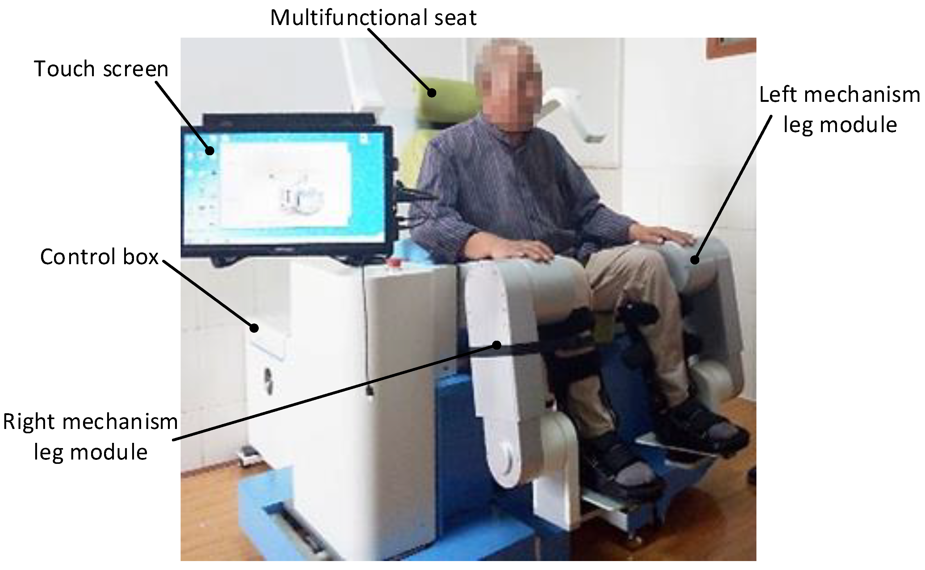
Abstract
:1. Introduction
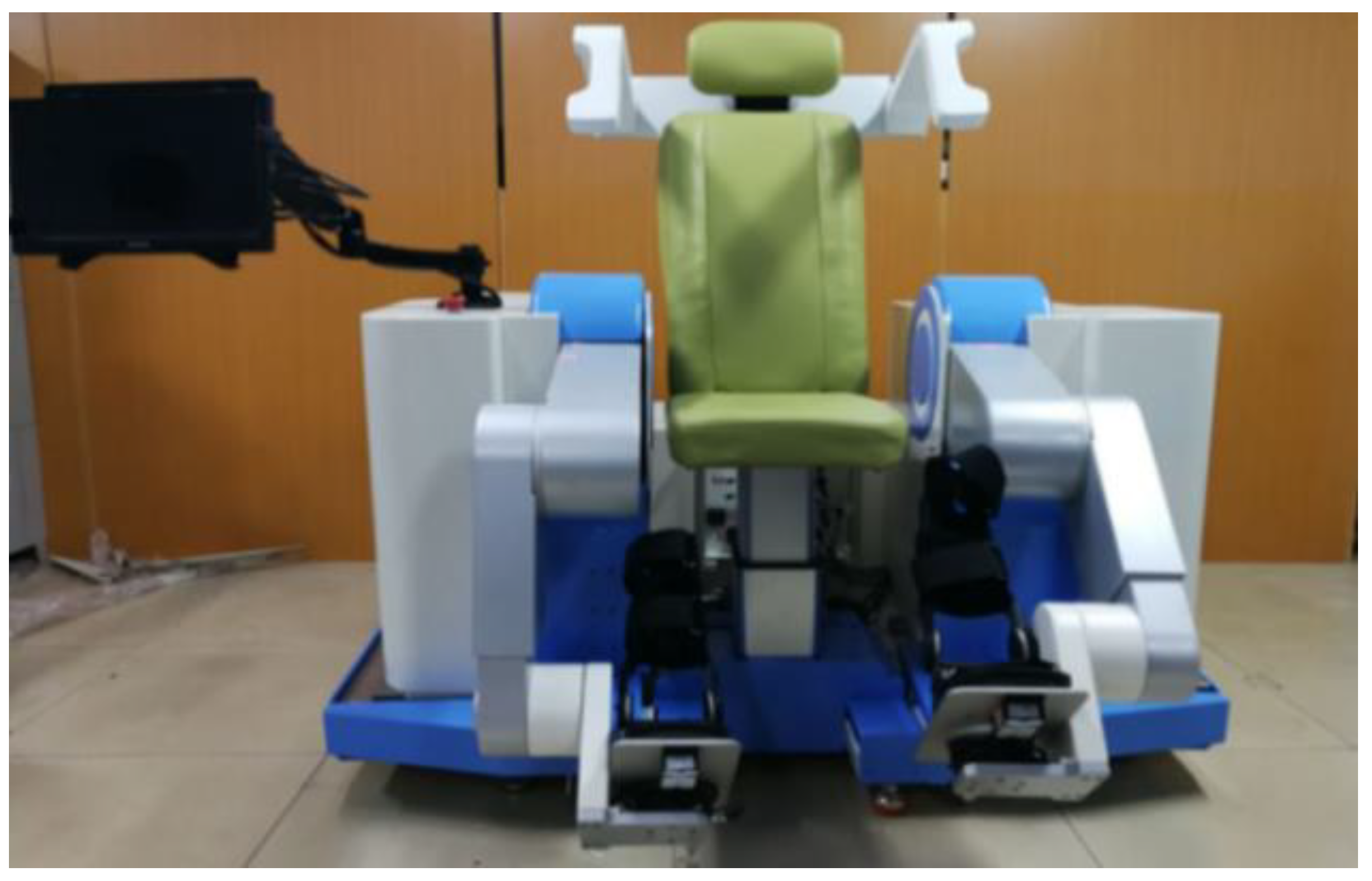
2. LLR-II Rehabilitation Robot
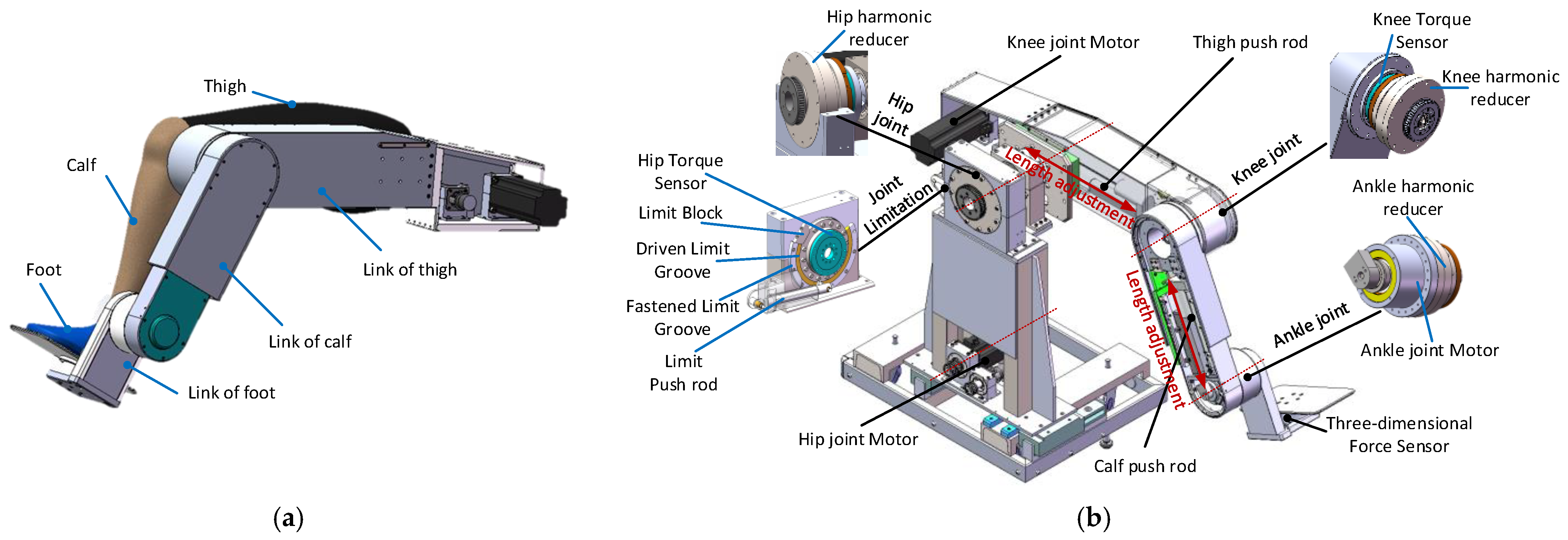
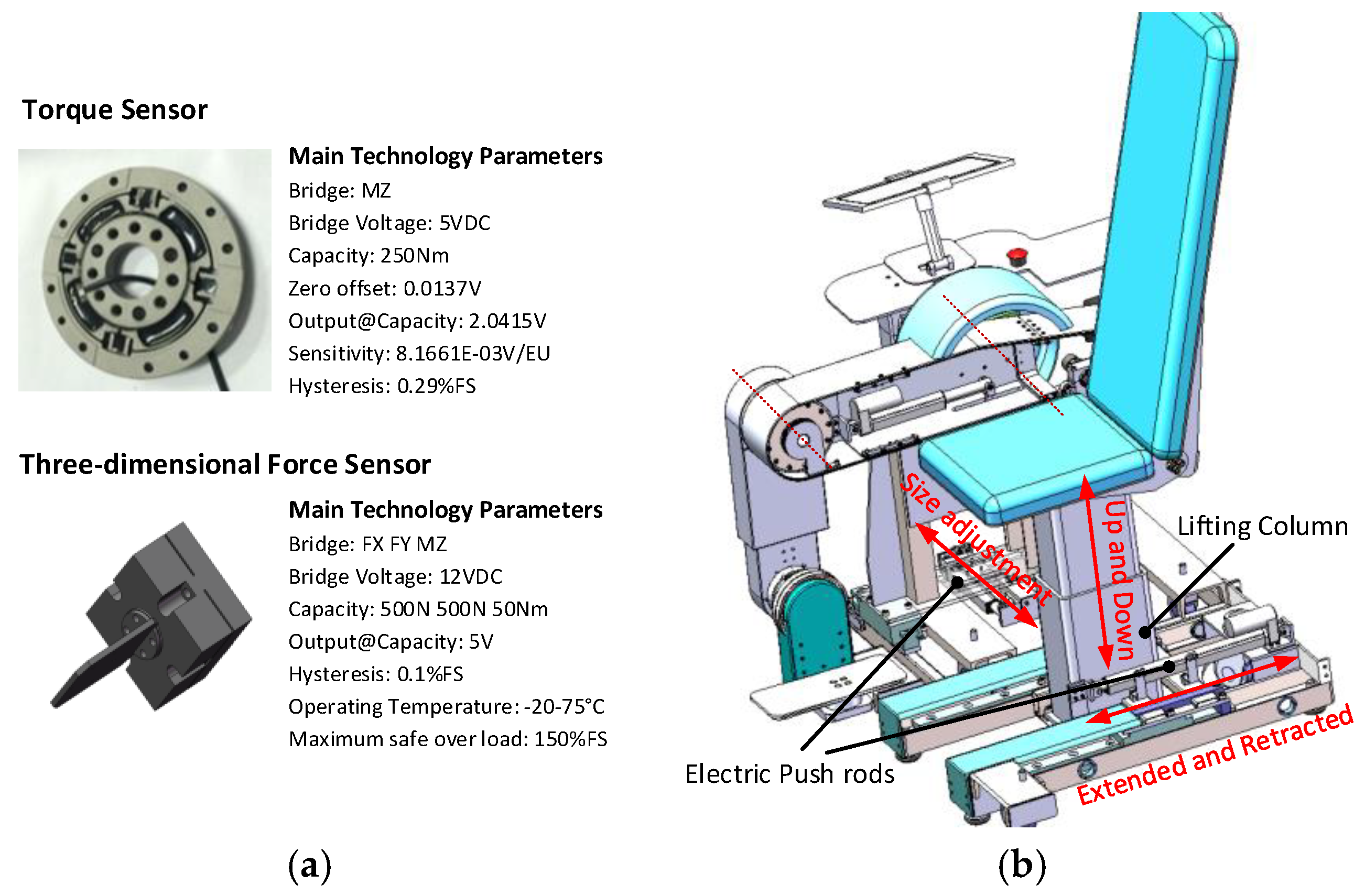
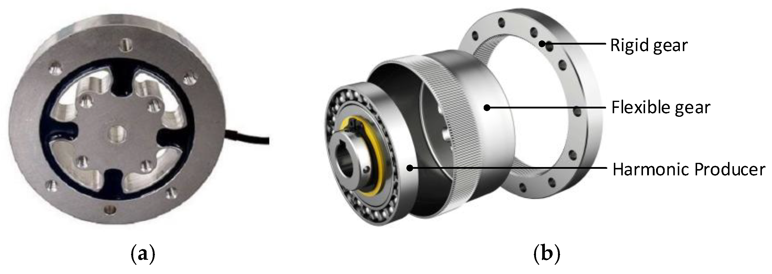
2.1. Structural Design and Electrical System
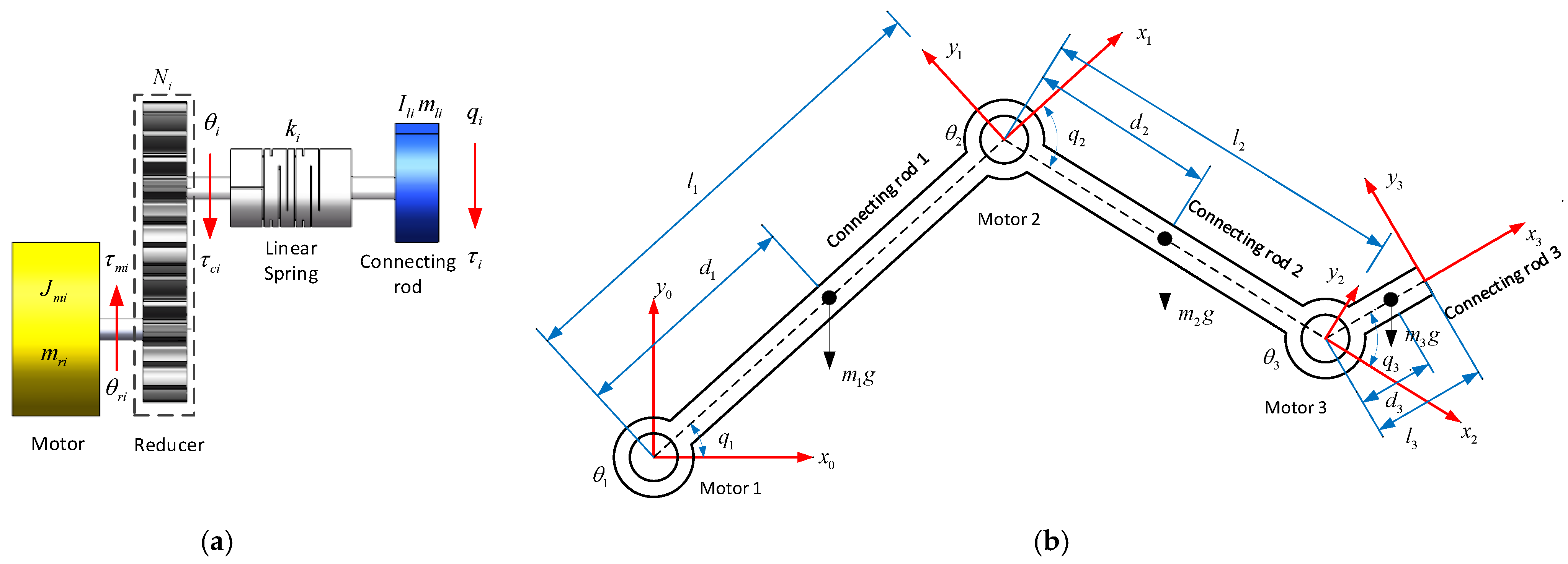
2.2. Human–Machine Interaction Mechanics Model Considering Joint Flexibility
2.2.1. Lagrange Functions Considering Joint Flexibility
- The motor rotor is an axisymmetric rigid body.
- The joint electrodynamics is fast enough compared with its mechanical dynamics, and the influence of motor dynamics is not considered in flexible joint model.
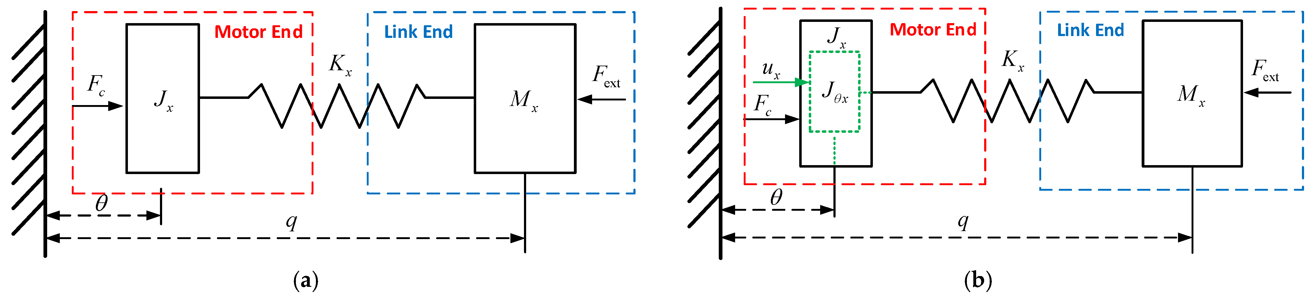
- Joint deformation is regarded as a linear torsion spring in the range of linear elasticity.
2.2.2. Dynamics Equation of Motor End Considering Joint Flexibility
2.2.3. Dynamics Equation of Link End Considering Joint Flexibility
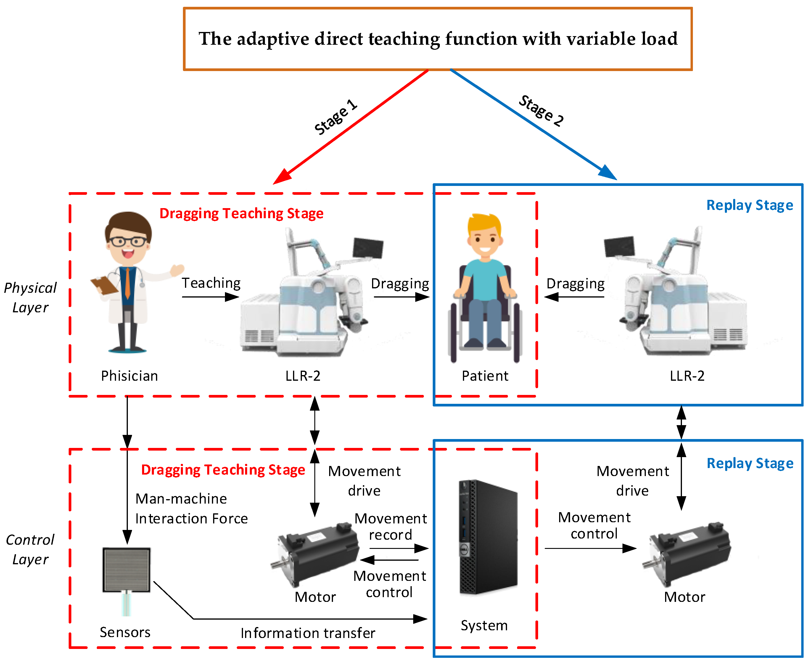
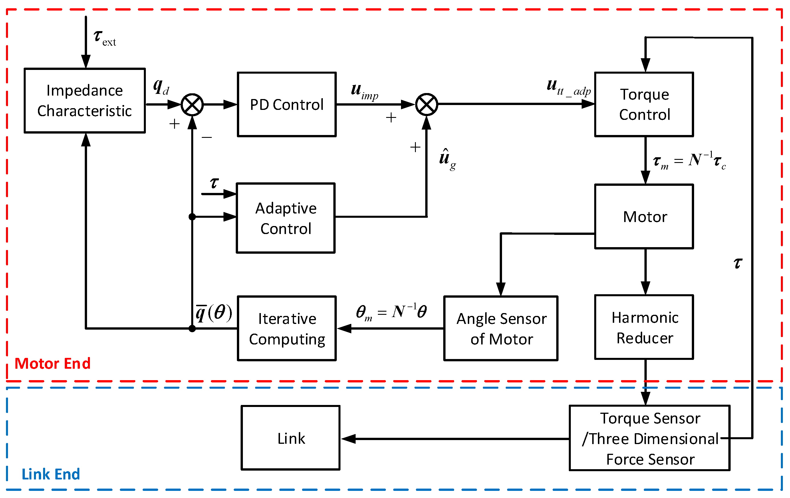
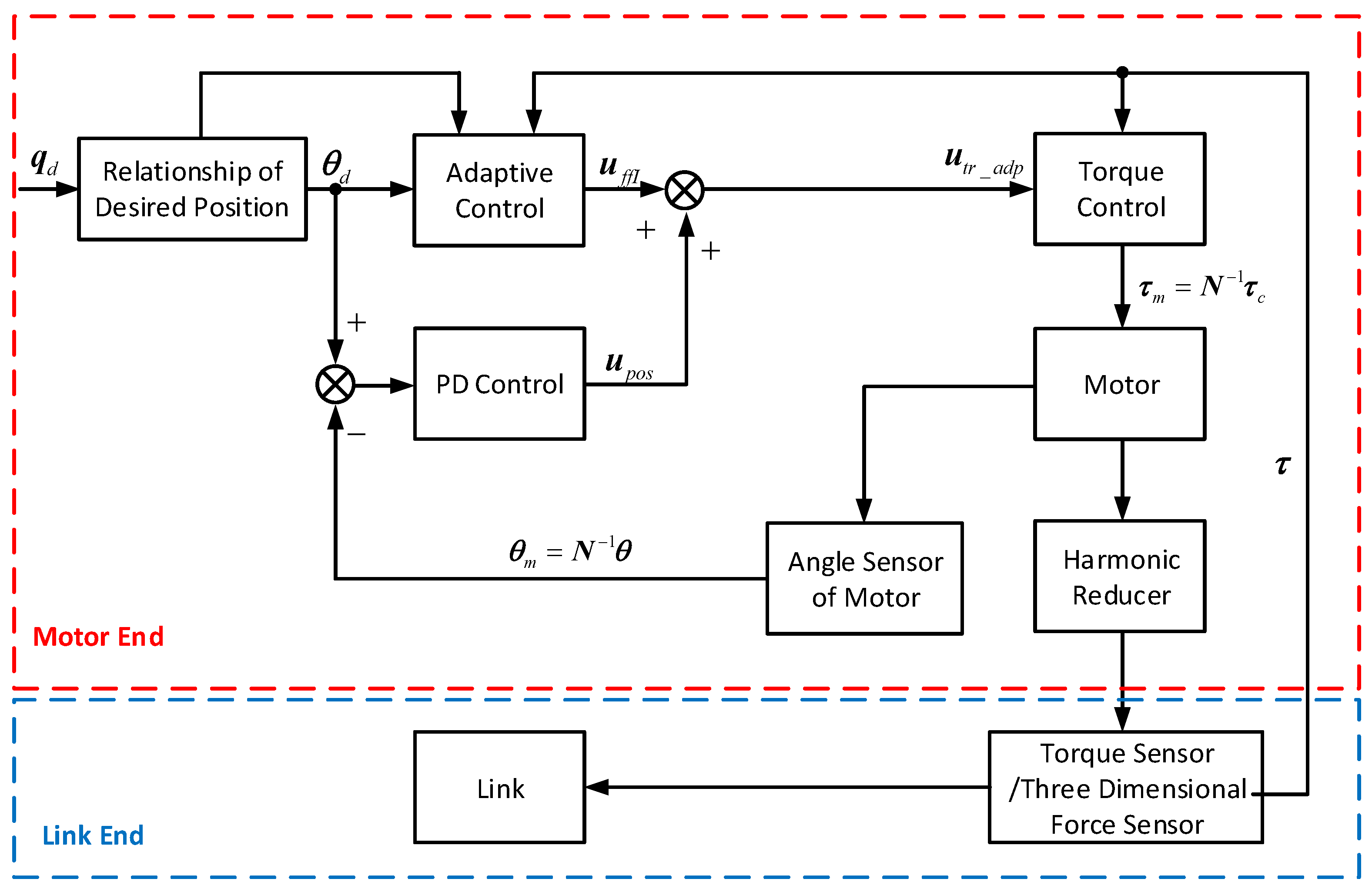
3. Control Law of the Adaptive Direct Teaching Function with Variable Load
3.1. Analysis of Factors Affecting Joint Flexibility and Ways of Intermediate Output Variables
3.2. Control Law of Dragging Teaching Stage
3.2.1. Control Law of Dragging Teaching Stage with No Load
3.2.2. Control Law of the Dragging Teaching Stage with Variable Load
3.2.3. Simulation of the Control Law of Dragging Teaching Stage
3.3. Control Law of the Replay Stage
3.3.1. Control Law of the Replay Stage with No Load
3.3.2. Control Law of the Replay Stage with Variable Load
3.3.3. Simulation of the Control Law in the Replay Stage
4. Experiment
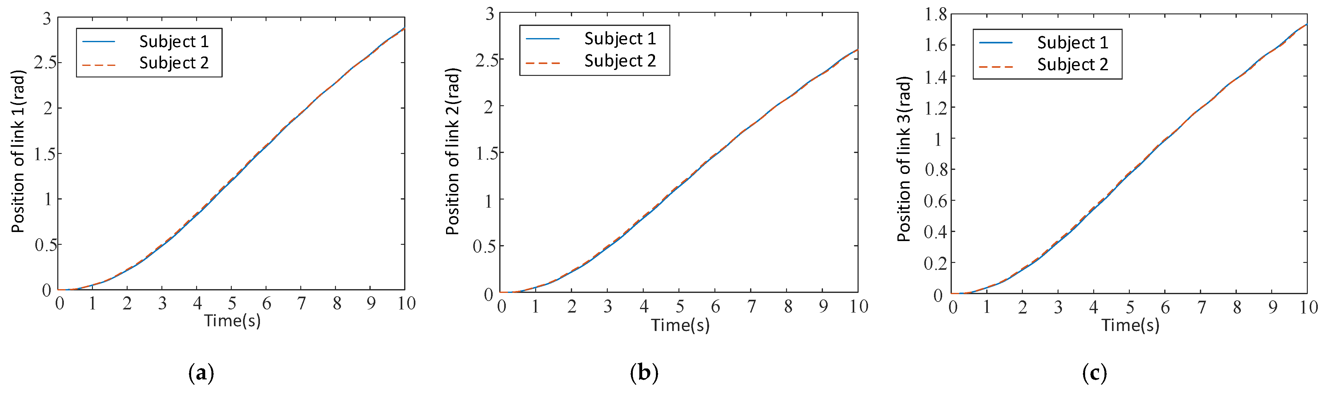
4.1. Experiment of Dragging Teaching Stage
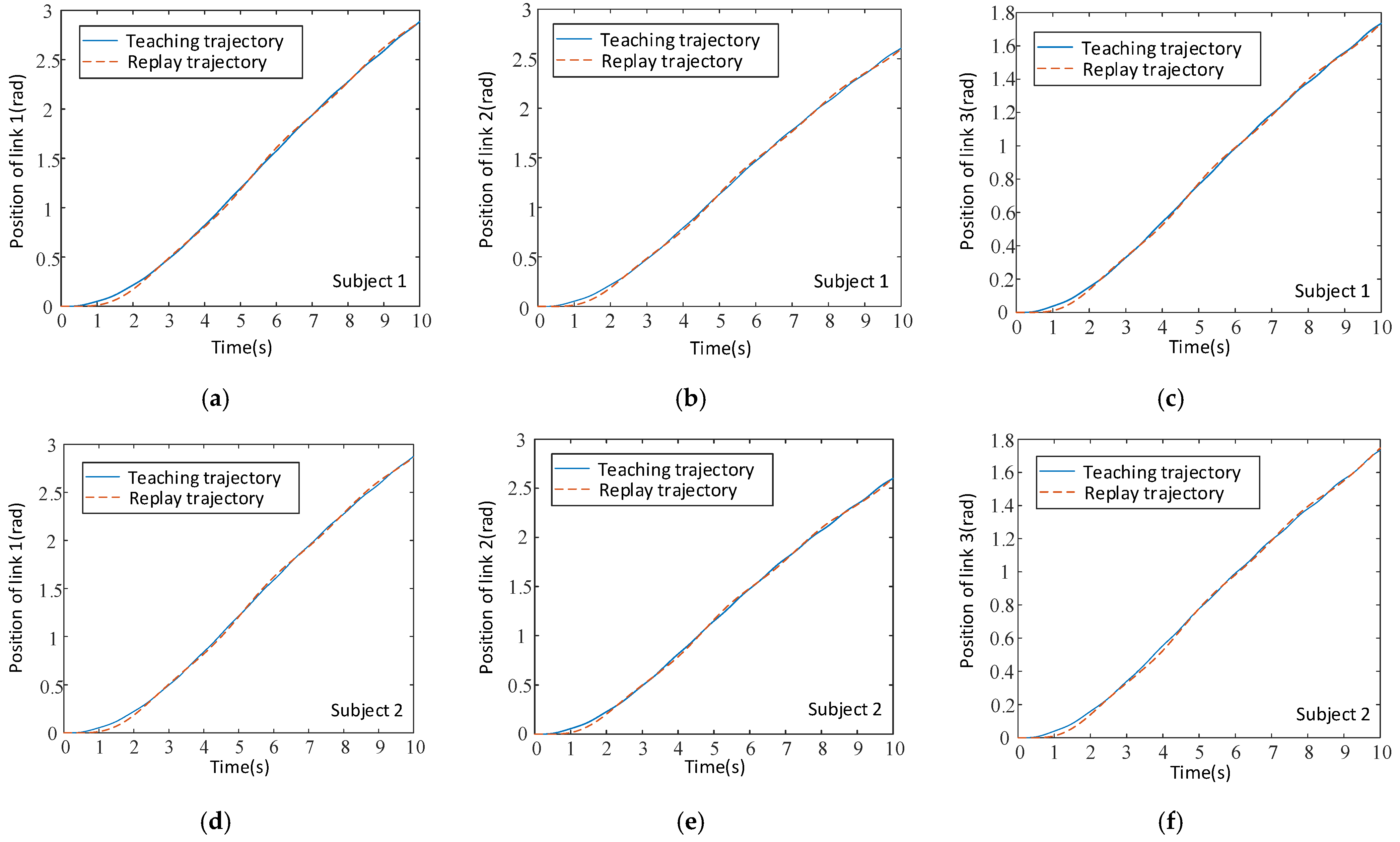
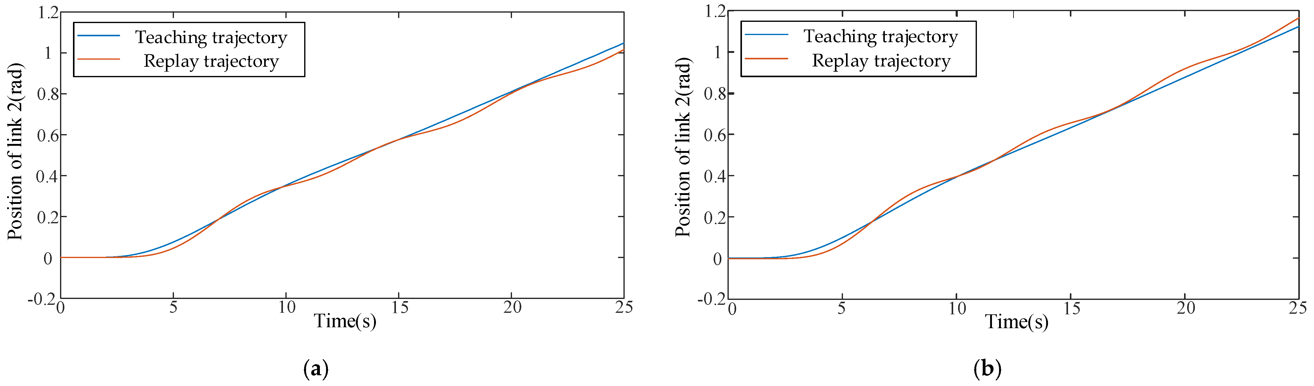
4.2. Experiment of the Replay Stage
5. Conclusions and Future Work
Author Contributions
Funding
Institutional Review Board Statement
Informed Consent Statement
Data Availability Statement
Conflicts of Interest
References
- Feigin, V.L.; Nguyen, G.; Cercy, K.; Johnson, C.O.; Alam, T.; Parmar, P.G.; Abajobir, A.A.; Abate, K.H.; Abd-Allah, F.; Abejie, A.N.; et al. Global, Regional, and Country-Specific Lifetime Risks of Stroke, 1990 and 2016. N. Engl. J. Med. 2018, 379, 2429–2437. [Google Scholar] [CrossRef]
- Feigin, V.L.; Mensah, G.A.; Norrving, B.; Murray, C.J.; Roth, G.A.; GBD 2013 Stroke Panel Experts Group. Atlas of the Global Burden of Stroke (1990–2013): The GBD 2013 Study. Neuroepidemiology 2015, 45, 230–236. [Google Scholar] [CrossRef] [PubMed]
- World Health Statistics 2020: Monitoring Health for the SDGs, Sustainable Development Goals. Available online: https://www.who.int/data/gho/publications/world-health-statistics (accessed on 26 April 2021).
- Koceska, N.; Koceski, S.; Durante, F.; Zobel, P.B.; Raparelli, T. Control architecture of a 10 dof lower limbs exoskeleton for gait rehabilitation. Int. J. Adv. Robot. Syst. 2013, 10, 68. [Google Scholar] [CrossRef] [Green Version]
- Meng, W.; Liu, Q.; Zhou, Z.D.; Ai, Q.S. Recent development of mechanisms and control strategies for robot-assisted lower limb rehabilitation. Mechatronics 2015, 31, 132–145. [Google Scholar] [CrossRef]
- Chen, K.; Zhang, Y.; Yi, J.; Liu, T. An integrated hysical-learning model of physical human-robot interactions with application to pose estimation in bikebot riding. Int. J. Robot. Res. 2016, 35, 1459–1476. [Google Scholar] [CrossRef]
- Gan, D.; Qiu, S.; Guan, Z.; Shi, C.; Li, Z. Development of an exoskeleton robot for lower limb rehabilitation. In Proceedings of the Conference on Advanced Robotics and Mechatronics, Macau, China, 18–20 August 2016; pp. 312–317. [Google Scholar] [CrossRef]
- Esquenazi, A.; Talaty, M.; Packel, A.; Saulino, M. The rewalk powered exoskeleton to restore ambulatory function to individuals with thoracic-level motor-complete spinal cord injury. Am. J. Phys. Med. Rehabil. 2012, 91, 911–921. [Google Scholar] [CrossRef] [PubMed] [Green Version]
- Fleerkotte, B.M.; Koopman, B.; Buurke, J.H.; van Asseldonk, E.H.; van der Kooij, H.; Rietman, J.S. The effffect of impedance-controlled robotic gait training on walking ability and quality in individuals with chronic incomplete spinal cord injury: An explorative study. J. Neuroeng. Rehabil. 2014, 11, 498–500. [Google Scholar] [CrossRef] [Green Version]
- Meuleman, J.; van Asseldonk, E.; van Oort, G.; Rietman, H.; van der Kooij, H. LOPES II—Design and evaluation of an admittance controlled gait training robot with shadow-leg approach. IEEE Trans. Neural Syst. Rehabil. Eng. 2016, 24, 352–363. [Google Scholar] [CrossRef]
- Koenig, A.; Riener, R. The human in the loop. In Neurorehabilitation Technology; Reinkensmeyer, D.J., Ed.; Springer: London, UK, 2016; pp. 161–181. [Google Scholar]
- Alcobendas-Maestro, M.; Esclarín-Ruz, A.; Casado-López, R.M.; Muñoz-González, A.; Perez-Mateos, G.; Gonzalez-Valdizan, E.; Martin, J.L. Lokomat robotic-assisted versus overground training within 3 to 6 months of incomplete spinal cord lesion: Randomized controlled trial. J. Neuroeng. Rehabil. 2012, 26, 1058–1063. [Google Scholar] [CrossRef]
- Bouri, M.; Abdi, E.; Bleuler, H.; Reynard, F.; Deriaz, O. Lower Limbs Robotic Rehabilitation Case Study with Clinical Trials. In Proceedings of the 2nd Workshop. on New Trends in Medical and Service Robotics, Belgrade, Serbia, 20 July 2013; pp. 31–44. [Google Scholar] [CrossRef]
- Wang, H.; Shi, X.; Liu, H.; Li, L.; Hou, Z.; Yu, H. Design, Kinematics, Simulation and Experiment for a Lower Limb Rehabilitation Robot. Proc. Inst. Mech. Eng. Part I J. Syst. Control Eng. 2011, 225, 860–872. [Google Scholar] [CrossRef]
- Chisholm, K.J.; Klumper, K.; Mullins, A.; Ahmadi, M. A task oriented haptic gait rehabilitation robot. Mechatronics 2014, 24, 1083–1091. [Google Scholar] [CrossRef]
- Bouri, M.; Gall, B.L.; Clavel, R. A new concept of parallel robot for rehabilitation and fifitness: The lambda. In Proceedings of the IEEE International Conference on Robotics and Biomimetics, Guilin, China, 12–23 December 2009; IEEE: New York, NY, USA, 2009; pp. 2503–2508. [Google Scholar] [CrossRef]
- Mayr, A.; Quirbach, E.; Picelli, A.; Koflfler, M.; Smania, N.; Saltuari, L. Early robot-assisted gait retraining in non-ambulatory patients with stroke: A single blind randomized controlled trial. Eur. J. Phys. Rehabil. Med. 2018, 54, 819–826. [Google Scholar] [CrossRef] [PubMed]
- Aurich-Schuler, T.; Gut, A.; Labruyere, R. The freed module for the lokomat facilitates a physiological movement pattern in healthy people—A proof of concept study. J. Neuroeng. Rehabil. 2019, 16, 1–13. [Google Scholar] [CrossRef]
- Akdogan, E.; Adli, M.A. The design and control of a therapeutic exercise robot for lower limb rehabilitation: Physiotherabot. Mechatronics 2011, 21, 509–522. [Google Scholar] [CrossRef]
- Métrailler, P.; Blanchard, V.; Perrin, I.; Brodard, R.; Clavel, R. Improvement of rehabilitation possibilities with the motionmaker TM. In Proceedings of the 1st IEEE/RAS-EMBS International Conf. on Biomedical Robotics and Biomechatronics, Pisa, Italy, 20–22 February 2006; pp. 359–364. [Google Scholar] [CrossRef]
- Feng, Y.; Wang, H.; Lu, T.; Vladareanuv, V.; Li, Q.; Zhao, C. Teaching Training Method of a Lower Limb Rehabilitation Robot. Int. J. Adv. Robot Syst. 2016, 13, 57–68. [Google Scholar] [CrossRef] [Green Version]
- Feng, Y.; Lu, T.; Du, Y.; Chen, F.; Li, Q.; Wang, H. Research on teaching training method of the lower limb rehabilitation robot. China Sci. 2016, 11, 1802–1807. [Google Scholar] [CrossRef]
- Zhao, X.; Lin, M.; Li, Q.; Shi, X.; Zhao, C.; Wang, H. Teaching and Training of the Lower Limb Rehabilitation Robot Based on Accelerometer. Chin. J. Sens. Actuators 2016, 29, 1596–1601. [Google Scholar]
- Guo, B.; Han, J.; Li, X.; Zhang, Y.; You, A. Personalized Gait Planning Method for the Lower-Limb Rehabilitation Training Robot with the Physiotherapist Interaction. Robot 2018, 40, 479–490. [Google Scholar] [CrossRef]
- Guo, B.; Han, J.; Li, X.; Wu, P.; Zhang, Y.; You, A. A wearable somatosensory teaching device with adjustable operating force for gait rehabilitation training robot. Adv. Mech. Eng. 2017, 9, 1–14. [Google Scholar] [CrossRef]
- Wang, H.; Feng, Y.; Yu, H.; Wang, Z.; Vladareanuv, V.; Du, Y. Mechanical design and trajectory planning of a lower limb rehabilitation robot with a variable workspace. Int. J. Adv. Robot Syst. 2018, 2018, 1–13. [Google Scholar] [CrossRef] [Green Version]
- Zhang, D. Research on Control System and Control Strategy of Lower Limbs Rehabilitation Robot. Master’s Thesis, Yanshan University, Qinhuangdao, China, May 2016. [Google Scholar]
- Emken, J.L.; Harkema, S.J.; Beres-Jones, J.A.; Ferreira, C.K.; Reinkensmeyer, D.J. Feasibility of Manual Teach-and-Replay and Continuous Impedance Shaping for Robotic Locomotor Training Following Spinal Cord Injury. IEEE Bio-Med. Eng. 2008, 55, 322–334. [Google Scholar] [CrossRef] [PubMed] [Green Version]
- Sun, J.G.; Gao, J.Y.; Zhang, J.H.; Tan, R.H. Teaching and playback control system for parallel robot for ankle joint rehabilitation. In Proceedings of the 2007 IEEE International Conference on Industrial Engineering and Engineering Management, Singapore, 2–4 December 2008. [Google Scholar] [CrossRef]
- Yang, H.; Han, J.; Li, X. Research on Drag and Teach of Horizontal Lower Limb Rehabilitative Robot. Mach. Des. Manuf. 2020, 5, 272–275. [Google Scholar] [CrossRef] [Green Version]
- Kugi, A.; Ott, C.; Albu-Schaffer, A.; Hirzinger, G. On the Passive-Based Impedance Control of Flexible Joint Robots. IEEE Robot 2008, 24, 416–429. [Google Scholar] [CrossRef]
- Hou, C.; Wang, Z.; Zhao, Y.; Song, G. Load Adaptive Force-free Control for the Direct Teaching of Robots. Robot 2017, 39, 439–448. [Google Scholar] [CrossRef]


Publisher’s Note: MDPI stays neutral with regard to jurisdictional claims in published maps and institutional affiliations. |
© 2021 by the authors. Licensee MDPI, Basel, Switzerland. This article is an open access article distributed under the terms and conditions of the Creative Commons Attribution (CC BY) license (https://creativecommons.org/licenses/by/4.0/).
Share and Cite
Wang, X.; Wang, H.; Hu, X.; Tian, Y.; Lin, M.; Yan, H.; Niu, J.; Sun, L. Adaptive Direct Teaching Control with Variable Load of the Lower Limb Rehabilitation Robot (LLR-II). Machines 2021, 9, 142. https://0-doi-org.brum.beds.ac.uk/10.3390/machines9080142
Wang X, Wang H, Hu X, Tian Y, Lin M, Yan H, Niu J, Sun L. Adaptive Direct Teaching Control with Variable Load of the Lower Limb Rehabilitation Robot (LLR-II). Machines. 2021; 9(8):142. https://0-doi-org.brum.beds.ac.uk/10.3390/machines9080142
Chicago/Turabian StyleWang, Xincheng, Hongbo Wang, Xinyu Hu, Yu Tian, Musong Lin, Hao Yan, Jianye Niu, and Li Sun. 2021. "Adaptive Direct Teaching Control with Variable Load of the Lower Limb Rehabilitation Robot (LLR-II)" Machines 9, no. 8: 142. https://0-doi-org.brum.beds.ac.uk/10.3390/machines9080142