
Classification Framework for Medical Diagnosis of Brain Tumor with an Effective Hybrid Transfer Learning Model

 , ,
, ,  , ,
, ,  ,
,
Abstract
:1. Introduction
- A precise Computer Aided Diagnosis system for BT is presented using deep learning.
- A new hybrid deep learning approach, GN-AlexNet, is introduced for the classification of three types of brain tumors (pituitary, meningioma, and glioma). The proposed CAD system is thoroughly tested on a publicly available benchmark dataset of Contrast-Enhanced magnetic resonance images (CE-MRI).
- In terms of accuracy and sensitivity, the proposed model performed significantly better than the existing techniques (with an accuracy of 99.51% and a sensitivity of 98.90%).
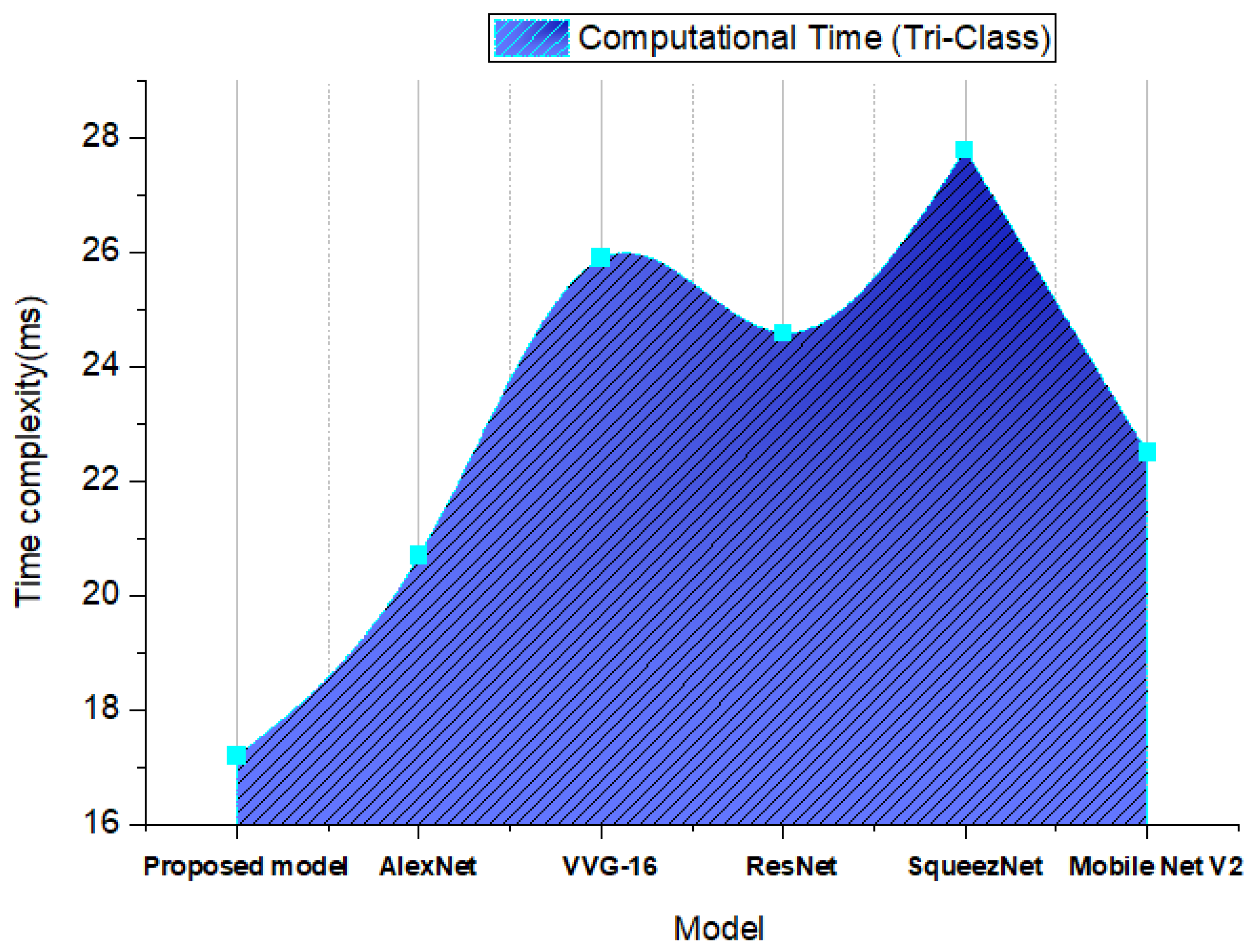
- High classification performance has been achieved with the suggested model, together with decreased time complexity (ms). The GA-AlexNet classifier is used for successful BTs diagnosis in clinical and biomedical research.
2. Literature Review
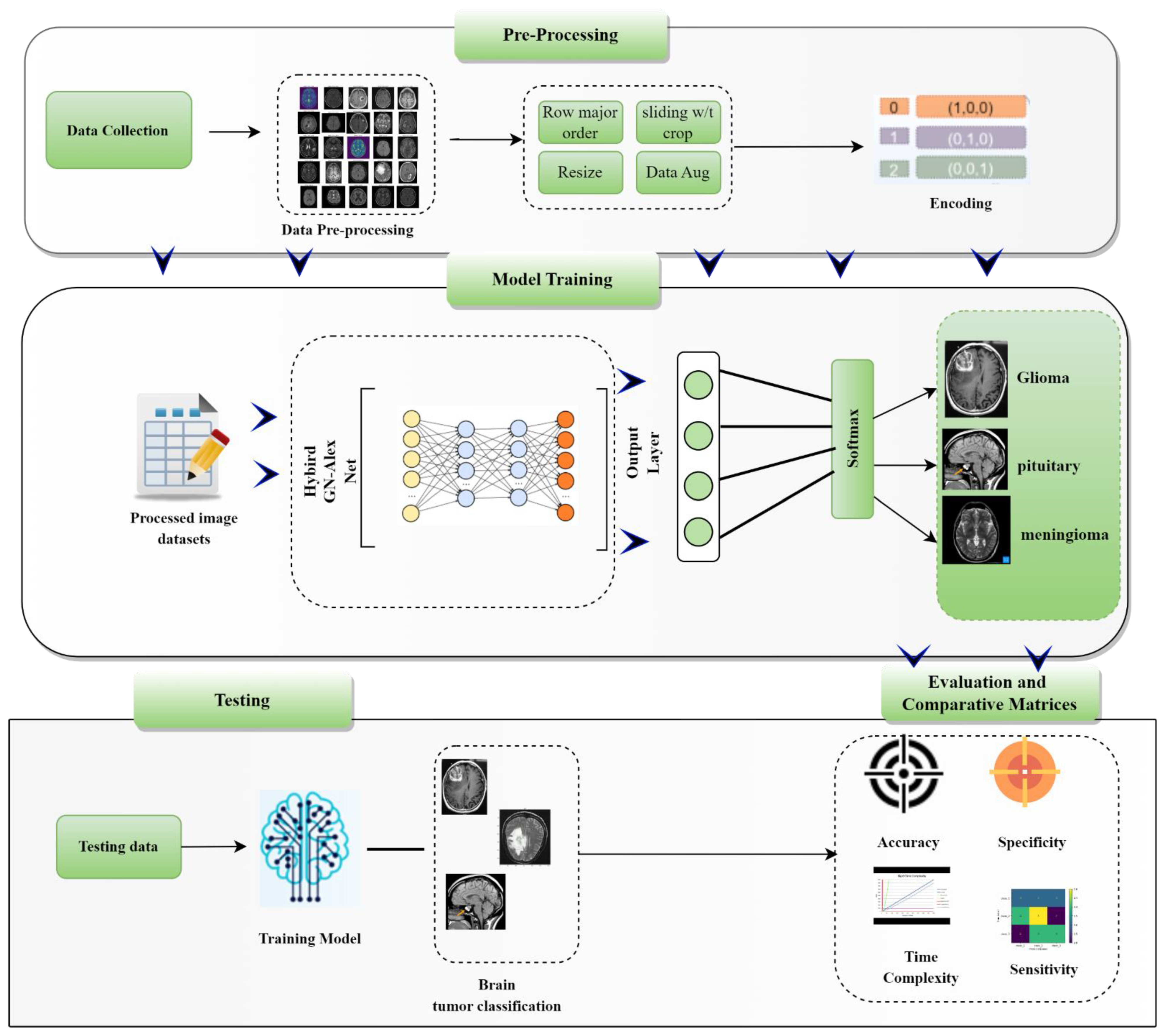
3. Methodology
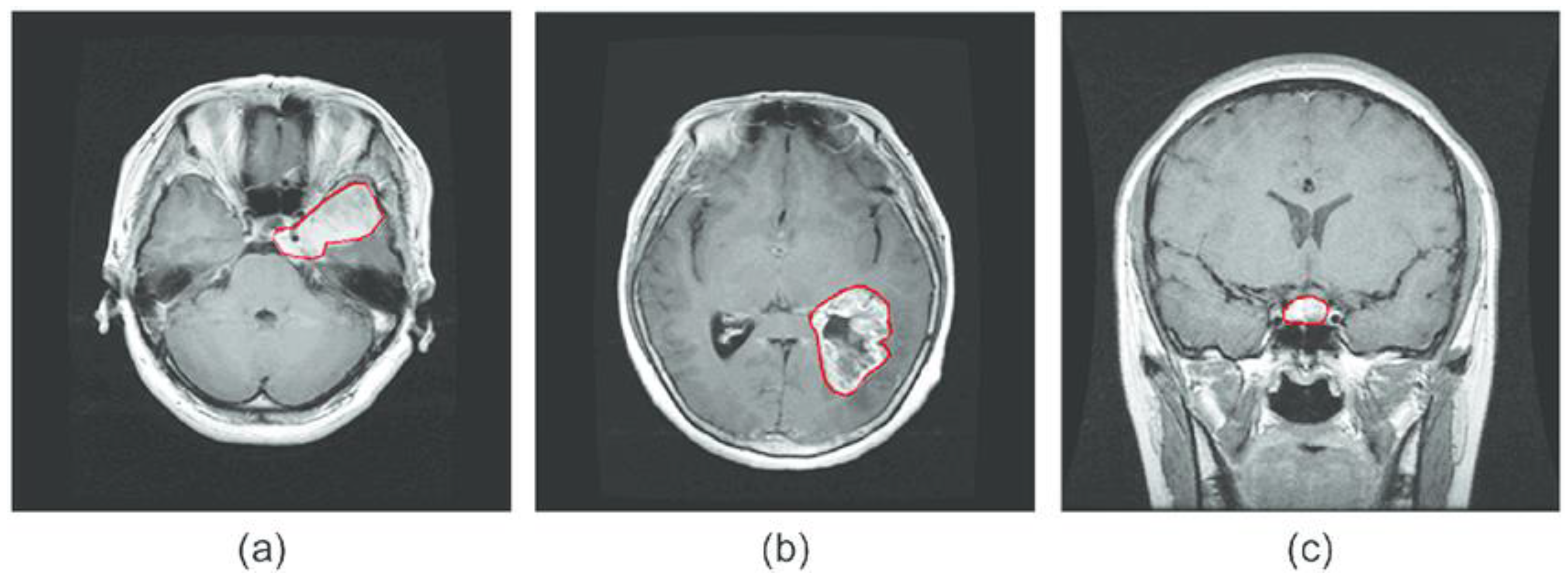
3.1. Brain Tumor CE-MRI Dataset
3.2. Data Preprocessing and Augmentation
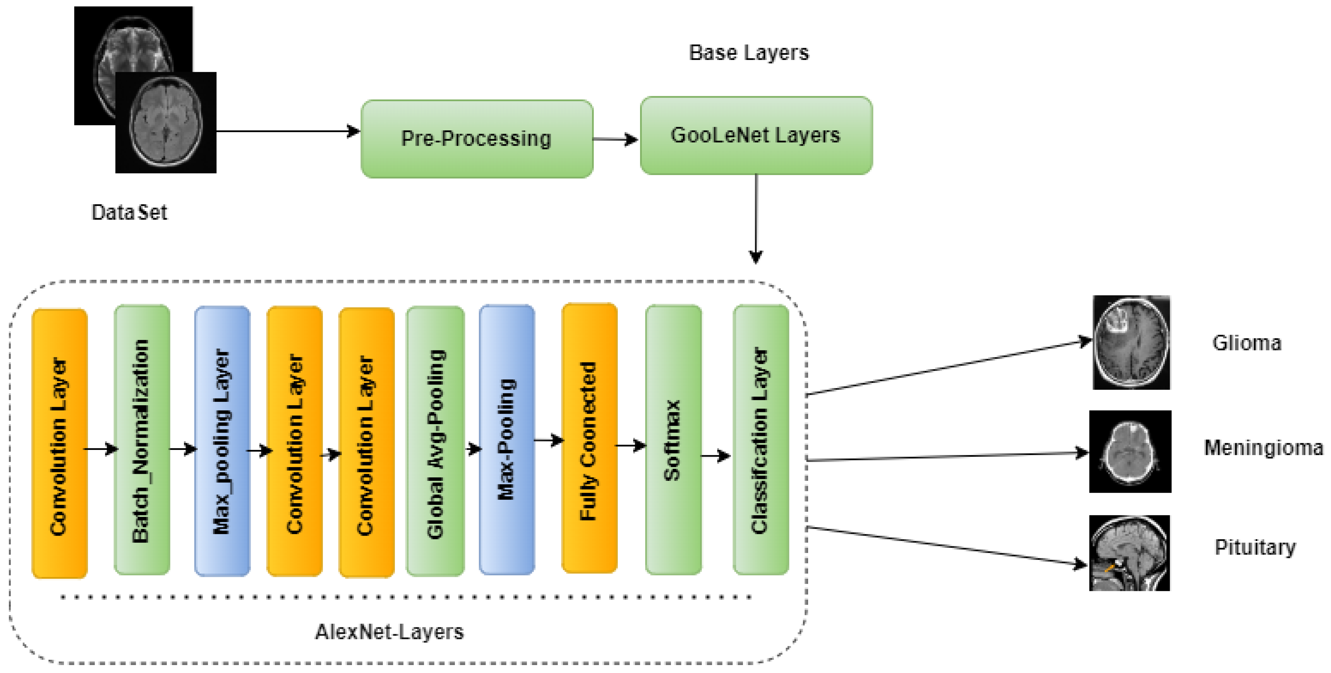
3.3. Proposed Model
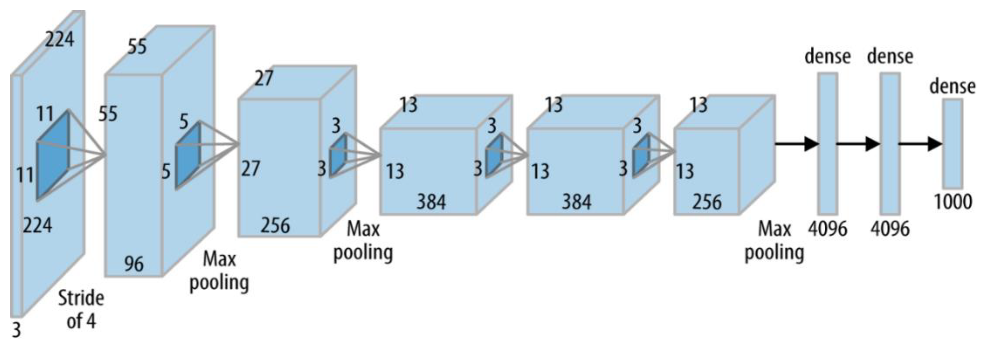
3.3.1. AlexNet
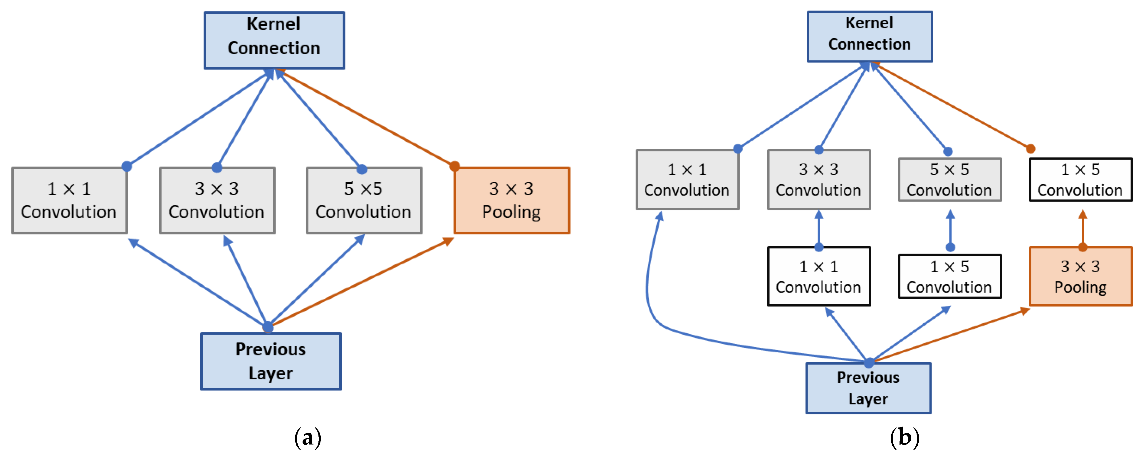
3.3.2. GoogleNeT
3.3.3. The Hybrid GN-AlexNet Deep Learning Model
3.4. Experimental Setup
3.5. Performance Evaluation Metrics
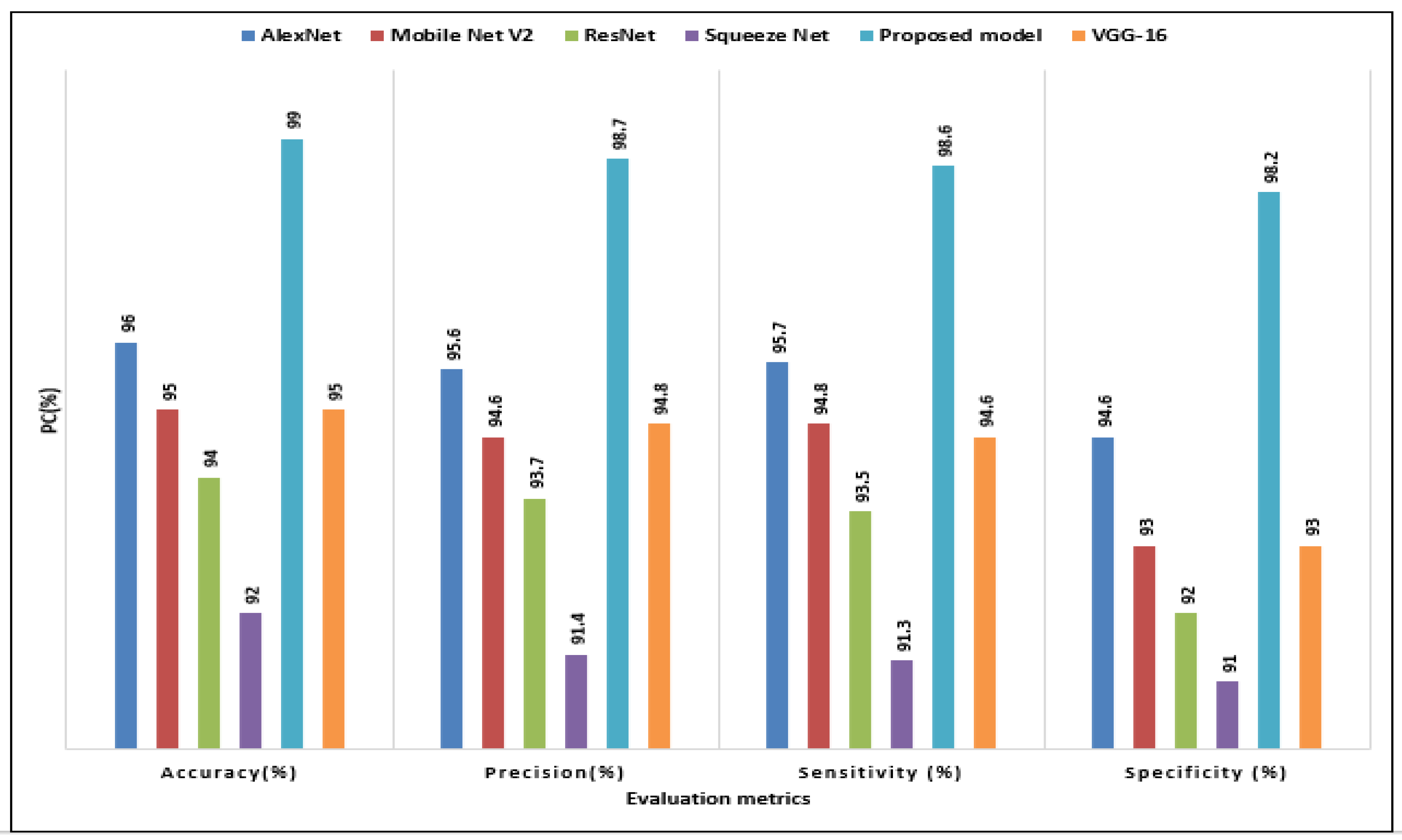
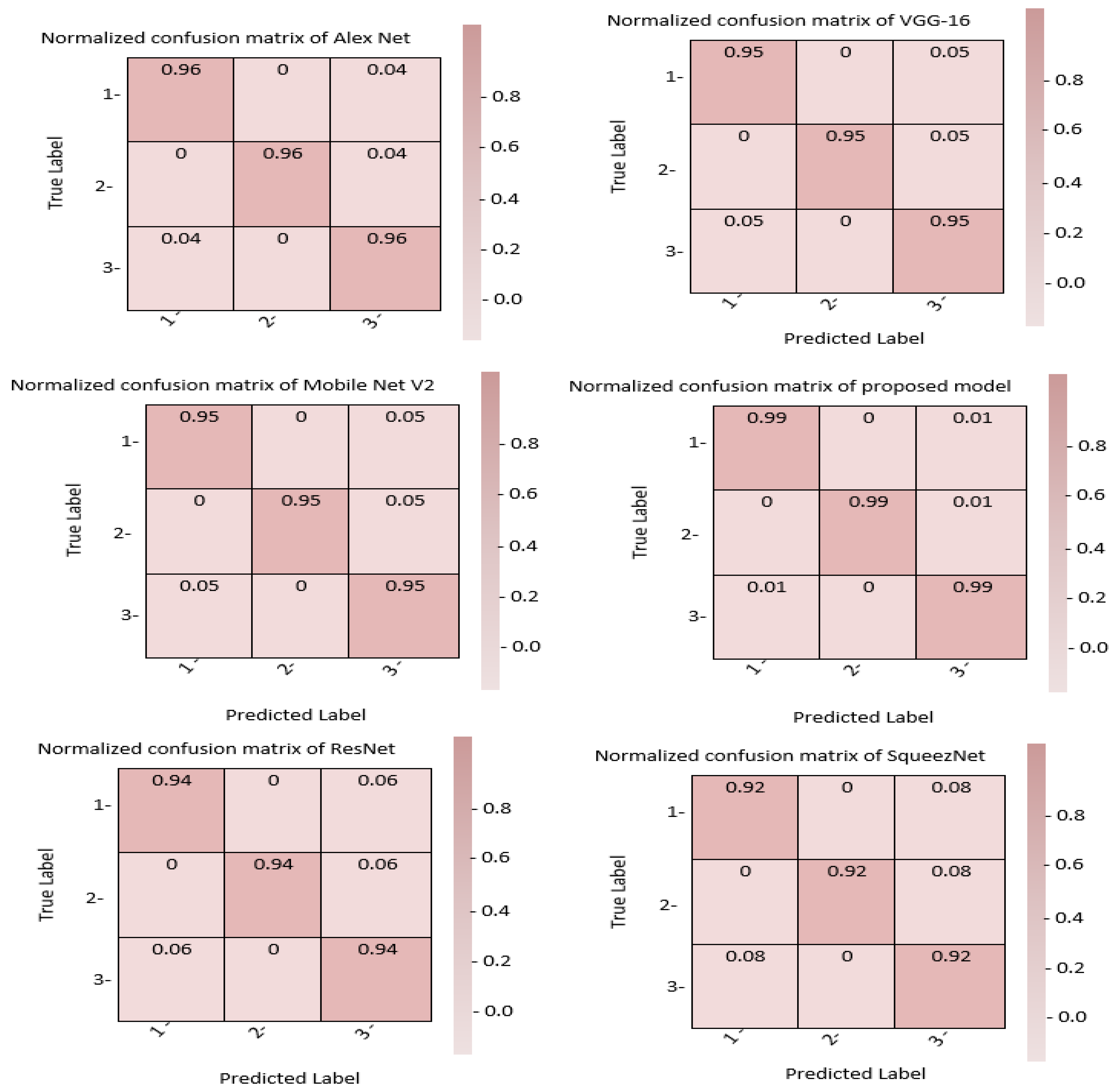
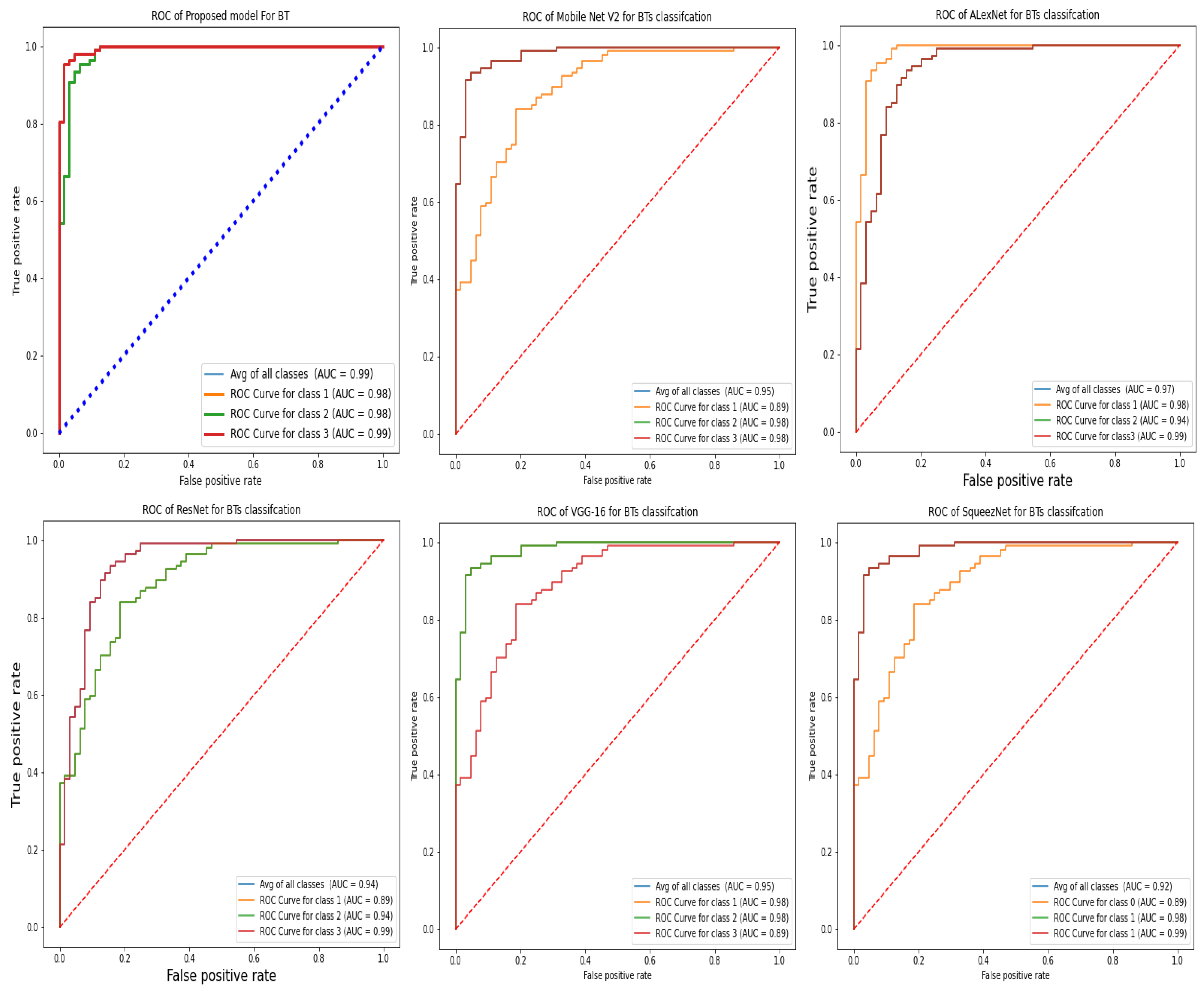
4. Result and Discussion
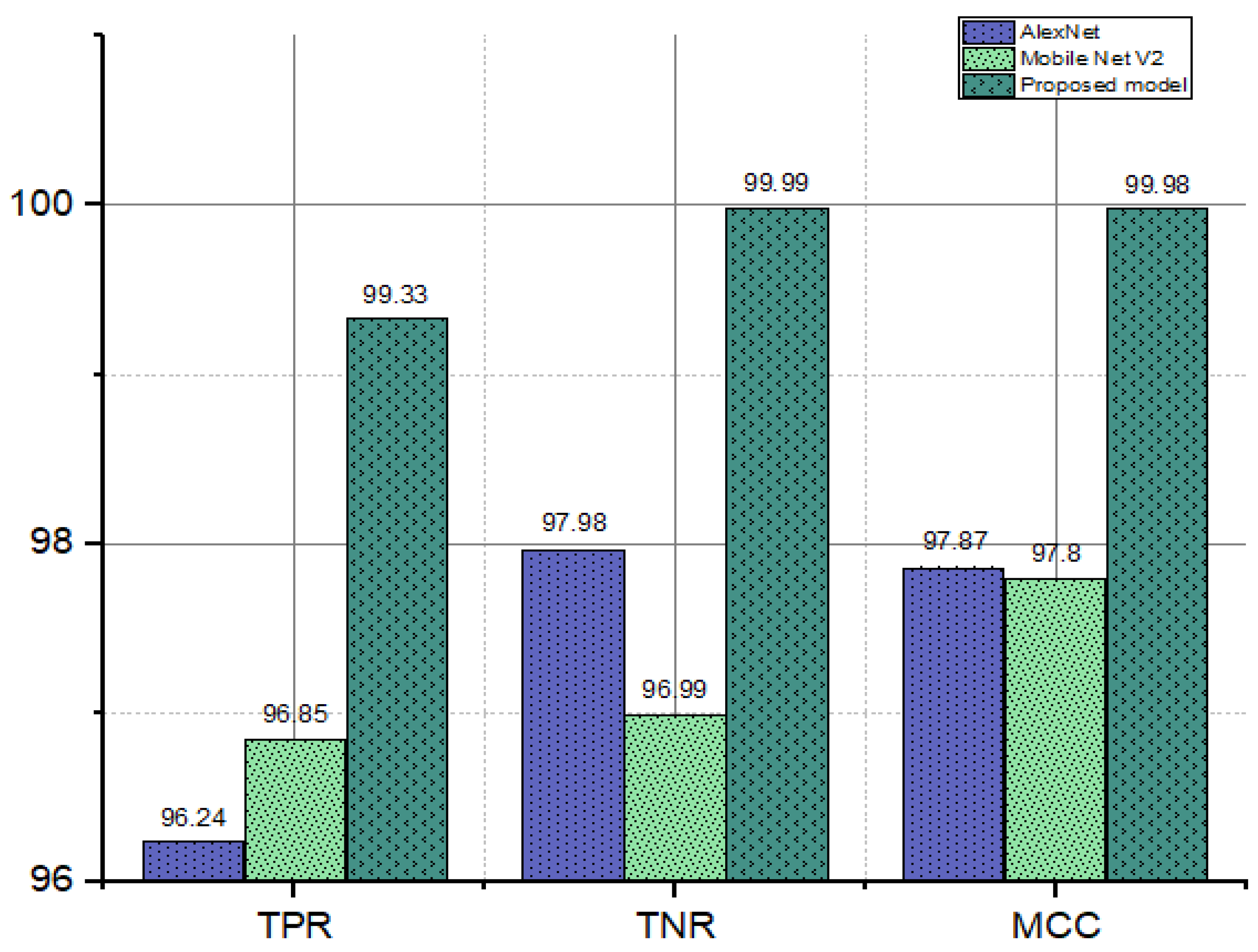
4.1. FDR, FNR, FOR, and FPR Analysis
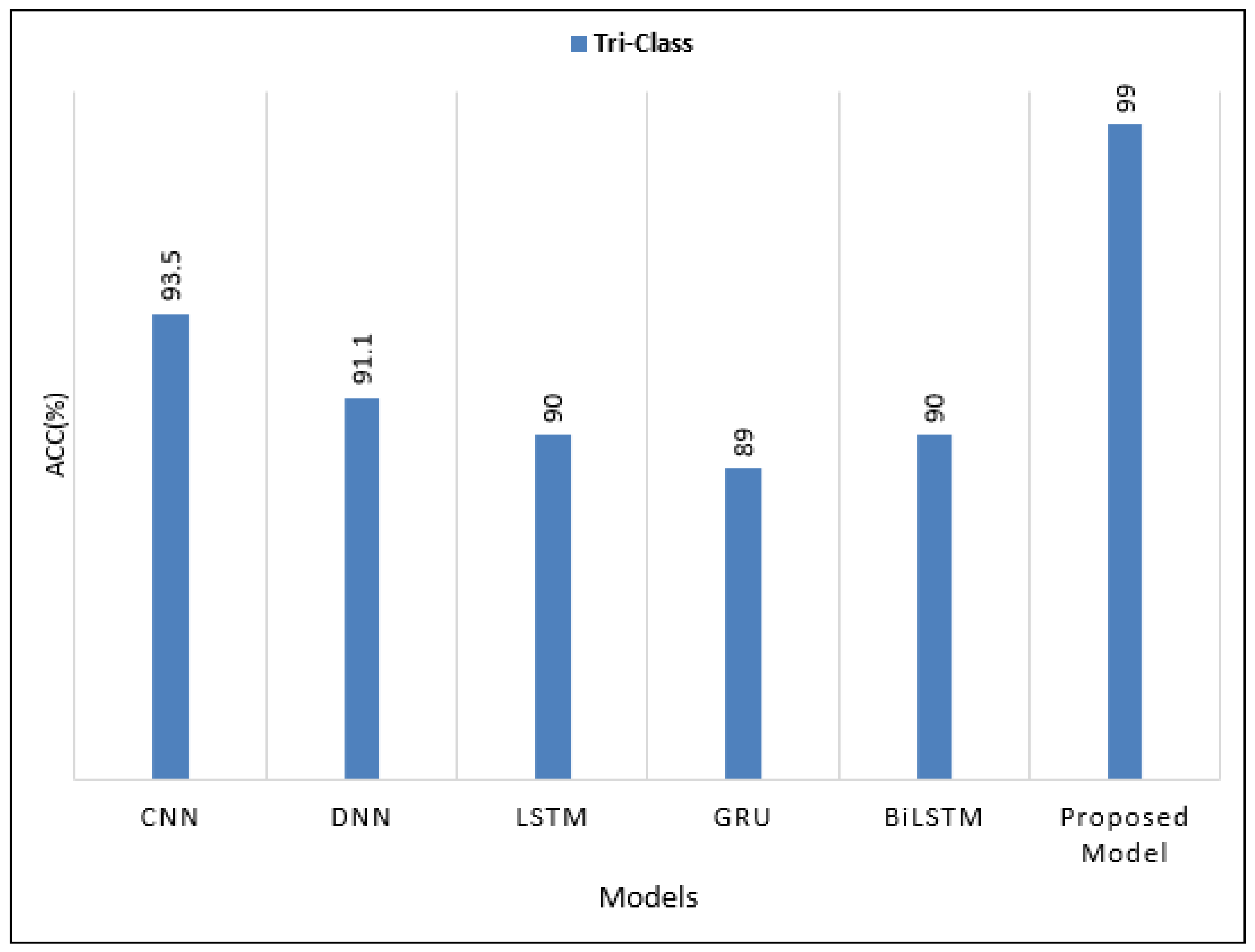
4.2. Comparative Results with Existing Benchmark
5. Conclusions
Author Contributions
Funding
Informed Consent Statement
Data Availability Statement
Acknowledgments
Conflicts of Interest
References
- Van Meir, E.G.; Hadjipanayis, C.G.; Norden, A.D.; Shu, H.K.; Wen, P.Y.; Olson, J.J. Exciting new advances in neuro-oncology: The avenue to a cure for malignant glioma. CA A Cancer J. Clin. 2010, 60, 166–193. [Google Scholar] [CrossRef] [PubMed] [Green Version]
- Shree, N.V.; Kumar, T.N. Identification and classification of BTMRI images with feature extraction using DWT and probabilistic neural network. Brain Inform. 2018, 5, 23–30. [Google Scholar] [CrossRef] [PubMed] [Green Version]
- Saddique, M.; Kazmi, J.H.; Qureshi, K. A hybrid approach of using symmetry technique for brain tumors. Comput. Math. Methods Med. 2014, 2014, 712783. [Google Scholar] [CrossRef] [PubMed]
- Komninos, J.; Vlassopoulou, V.; Protopapa, D.; Korfias, S.; Kontogeorgos, G.; Sakas, D.E.; Thalassinos, N.C. Tumors are metastatic to the pituitary gland: Case report and literature review. J. Clin. Endocrinol. Metab. 2004, 2, 574–580. [Google Scholar] [CrossRef] [Green Version]
- DeAngelis, L.M. Brain tumors. N. Engl. J. Med. 2001, 344, 114–123. [Google Scholar] [CrossRef] [PubMed] [Green Version]
- Louis, D.N.; Perry, A.; Reifenberger, G.; Von Deimling, A.; Figarella-Branger, D.; Cavenee, W.K.; Ohgaki, H.; Wiestler, O.D.; Kleihues, P.; Ellison, D.W. The 2016 World Health Organization classification of tumors of the central nervous system: A summary. Acta Neuropathol. 2016, 132, 803–820. [Google Scholar] [CrossRef] [PubMed] [Green Version]
- Chahal, P.K.; Pandey, S.; Goel, S. A survey on brain tumors detection techniques for MR images. Multimed. Tools Appl. 2020, 79, 21771–21814. [Google Scholar] [CrossRef]
- Sajjad, M.; Khan, S.; Muhammad, K.; Wu, W.; Ullah, A.; Baik, S.W. Multi-grade brain tumors classification using deep CNN with extensive data augmentation. J. Comput. Sci. 2019, 30, 174–182. [Google Scholar] [CrossRef]
- Rehman, A.; Naz, S.; Razzak, M.I.; Akram, F.; Imran, M. A deep learning-based framework for automatic brain tumors classification using transfer learning. Circuits Syst. Signal Process. 2020, 39, 757–775. [Google Scholar] [CrossRef]
- Wang, Y.; Zu, C.; Hu, G.; Luo, Y.; Ma, Z.; He, K.; Wu, X.; Zhou, J. Automatic tumor segmentation with deep convolutional neural networks for radiotherapy applications. Neural Process. Lett. 2018, 48, 1323–1334. [Google Scholar] [CrossRef]
- Jégou, S.; Drozdzal, M.; Vazquez, D.; Romero, A.; Bengio, Y. The one hundred layers tiramisu: Fully convolutional denseness for semantic segmentation. In Proceedings of the IEEE Conference on Computer Vision and Pattern Recognition Workshops, Honolulu, HI, USA, 21–26 July 2017; pp. 11–19. [Google Scholar]
- Zhang, Q.; Cui, Z.; Niu, X.; Geng, S.; Qiao, Y. Image segmentation with pyramid dilated convolution based on ResNet and U-Net. In Proceedings of the International Conference on Neural Information Processing, Guangzhou, China, 14 November 2017; pp. 364–372. [Google Scholar]
- Raza, A.; Ayub, H.; Khan, J.A.; Ahmad, I.; Salama, S.A.; Daradkeh, Y.I.; Javeed, D.; Ur Rehman, A.; Hamam, H. A Hybrid Deep Learning-Based Approach for Brain Tumor Classification. Electronics 2022, 11, 1146. [Google Scholar] [CrossRef]
- Ding, Y.; Zhang, C.; Lan, T.; Qin, Z.; Zhang, X.; Wang, W. Classification of Alzheimer’s disease based on the combination of morphometric feature and texture feature. In Proceedings of the 2015 IEEE International Conference on Bioinformatics and Biomedicine (BIBM), Washington, DC, USA, 9–12 November 2015; pp. 409–412. [Google Scholar]
- Samee, N.A.; Atteia, G.; Meshoul, S.; Al-Antari, M.A.; Kadah, Y.M. Deep Learning Cascaded Feature Selection Framework for Breast Cancer Classification: Hybrid CNN with Univariate-Based Approach. Mathematics 2022, 10, 3631. [Google Scholar] [CrossRef]
- Szegedy, C.; Liu, W.; Jia, Y.; Sermanet, P.; Reed, S.; Anguelov, D.; Erhan, D.; Vanhoucke, V.; Rabinovich, A. Going deeper with convolutions. In Proceedings of the IEEE Conference on Computer Vision and Pattern Recognition, Boston, MA, USA, 7–12 June 2015; pp. 1–9. [Google Scholar]
- Harish, P.; Baskar, S. MRI based detection and classification of brain tumor using enhanced faster R-CNN and Alex Net model. Mater. Today Proc. 2020, 11, 495. [Google Scholar] [CrossRef]
- Ijaz, A.; Ullah, I.; Khan, W.U.; Ur Rehman, A.; Adrees, M.S.; Saleem, M.Q.; Cheikhrouhou, O.; Hamam, H.; Shafiq, M. Efficient algorithms for E-healthcare to solve multiobject fuse detection problem. J. Healthc. Eng. 2021, 2021, 9500304. [Google Scholar]
- Ahmad, I.; Liu, Y.; Javeed, D.; Ahmad, S. A decision-making technique for solving order allocation problem using a genetic algorithm. IOP Conf. Ser. Mater. Sci. Eng. 2020, 853, 012054. [Google Scholar] [CrossRef]
- Binaghi, E.; Omodei, M.; Pedoia, V.; Balbi, S.; Lattanzi, D.; Monti, E. Automatic segmentation of MR brain tumors images using support vector machine in combination with graph cut. In Proceedings of the 6th International Joint Conference on Computational Intelligence (IJCCI), Rome, Italy, 22–24 October 2014; pp. 152–157. [Google Scholar]
- Wang, X.; Ahmad, I.; Javeed, D.; Zaidi, S.A.; Alotaibi, F.M.; Ghoneim, M.E.; Daradkeh, Y.I.; Asghar, J.; Eldin, E.T. Intelligent Hybrid Deep Learning Model for Breast Cancer Detection. Electronics 2022, 11, 2767. [Google Scholar] [CrossRef]
- Ahmad, S.; Ullah, T.; Ahmad, I.; Al-Sharabi, A.; Ullah, K.; Khan, R.A.; Rasheed, S.; Ullah, I.; Uddin, M.; Ali, M. A novel hybrid deep learning model for metastatic cancer detection. Comput. Intell. Neurosci. 2022, 2022, 8141530. [Google Scholar] [CrossRef] [PubMed]
- Ahmad, I.; Wang, X.; Zhu, M.; Wang, C.; Pi, Y.; Khan, J.A.; Khan, S.; Samuel, O.W.; Chen, S.; Li, G. EEG-based epileptic seizure detection via machine/deep learning approaches: A Systematic Review. Comput. Intell. Neurosci. 2022, 2022, 6486570. [Google Scholar] [CrossRef] [PubMed]
- Ullah, N.; Khan, J.A.; Alharbi, L.A.; Raza, A.; Khan, W.; Ahmad, I. An Efficient Approach for Crops Pests Recognition and Classification Based on Novel DeepPestNet Deep Learning Model. IEEE Access 2022, 10, 73019–73032. [Google Scholar] [CrossRef]
- Tufail, A.B.; Ullah, I.; Khan, W.U.; Asif, M.; Ahmad, I.; Ma, Y.K.; Khan, R.; Ali, M. Diagnosis of diabetic retinopathy through retinal fundus images and 3D convolutional neural networks with limited number of samples. Wirel. Commun. Mob. Comput. 2021, 2021, 6013448. [Google Scholar] [CrossRef]
- Khan, H.A.; Jue, W.; Mushtaq, M.; Mushtaq, M.U. Brain tumour classification in MRI image using convolutional neural network. Math. Biosci. Eng. 2020, 17, 6203–6216. [Google Scholar] [CrossRef] [PubMed]
- Amin, J.; Sharif, M.; Haldorai, A.; Yasmin, M.; Nayak, R.S. Brain tumour detection and classification using machine learning: A comprehensive survey. Complex Intell. Syst. 2021, 8, 3161–3183. [Google Scholar] [CrossRef]
- Srivastava, N.; Hinton, G.E.; Sutskever, I. A simple way to prevent neural networks from over fitting. J. Mach. Learn. Res. 2014, 15, 1929–1958. Available online: https://www.jmlr.org/papers/volume15/srivastava14a/srivastava14a.pdf (accessed on 10 September 2022).
- Dvorák, P.; Menze, B. Structured prediction with convolutional neural networks for multimodal brain tumour segmentation. In Proceedings of the MICCAI Multimodal Brain Tumour Segmentation Challenge (BraTS), Munich, Germany, 5–9 October 2015; pp. 13–24. Available online: http://people.csail.mit.edu/menze/papers/dvorak_15_cnnTumor.pdf (accessed on 10 September 2022).
- Irsheidat, S.; Duwairi, R. Brain Tumour Detection Using Artificial Convolutional Neural Networks. In Proceedings of the 2020 11th International Conference on Information and Communication Systems (ICICS), Irbid, Jordan, 7–9 April 2020; pp. 197–203. [Google Scholar] [CrossRef]
- Sravya, V.; Malathi, S. Survey on Brain Tumour Detection using Machine Learning and Deep Learning. In Proceedings of the 2021 International Conference on Computer Communication and Informatics (ICCCI), Coimbatore, India, 27–29 January 2021; pp. 1–3. [Google Scholar] [CrossRef]
- Dipu, N.M.; Shohan, S.A.; Salam, K.M.A. Deep Learning Based Brain Tumour Detection and Classification. In Proceedings of the 2021 International Conference on Intelligent Technologies (CONIT), Hubli, India, 25–27 June 2021; pp. 1–6. [Google Scholar] [CrossRef]
- Gaikwad, S.; Patel, S.; Shetty, A. Brain Tumour Detection: An Application Based on Machine Learning. In Proceedings of the 2021 2nd International Conference for Emerging Technology (INCET), Belagavi, India, 21–23 May 2021; pp. 1–4. [Google Scholar] [CrossRef]
- Khairandish, M.O.; Sharma, M.; Jain, V.; Chatterjee, J.M.; Jhanjhi, N.Z. A hybrid CNN-SVM threshold segmentation approach for tumor detection and classification of MRI brain images. IRBM 2021, 43, 290–299. [Google Scholar] [CrossRef]
- Swati, Z.N.K.; Zhao, Q.; Kabir, M.; Ali, F.; Ali, Z.; Ahmed, S.; Lu, J. Brain tumors classification for MR images using transferlearning and fine-tuning. Comput. Med. Imaging Graph. 2019, 75, 34–46. [Google Scholar] [CrossRef] [PubMed]
- Kumar, S.; Mankame, D.P. Optimization drove deep convolution neural network for brain tumors classification. Biocybern. Biomed. Eng. 2020, 40, 1190–1204. [Google Scholar] [CrossRef]
- Deepak, S.; Ameer, P.M. Brain tumors classification using in-depth CNN features via transfer learning. Comput. Biol. Med. 2019, 111, 103345. [Google Scholar] [CrossRef] [PubMed]
- Raja, P.S. Brain tumors classification using a hybrid deep autoencoder with Bayesian fuzzy clustering-based segmentation approach. Biocybern. Biomed. Eng. 2020, 40, 440–453. [Google Scholar] [CrossRef]
- Ramamurthy, D.; Mahesh, P.K. Whale Harris Hawks optimization-based deep learning classifier for brain tumors detection using MRI images. J. King Saud Univ. Comput. Inf. Sci. 2020, 32, 1–14. [Google Scholar]
- Bahadure, N.B.; Ray, A.K.; Thethi, H.P. Image analysis for MRI-based brain tumors detection and feature extraction using biologically inspired BWT and SVM. Int. J. Biomed. Imaging 2017, 2017, 9749108. [Google Scholar] [CrossRef] [PubMed] [Green Version]
- Waghmare, V.K.; Kolekar, M.H. Brain tumors classification using deep learning. In The Internet of Things for Healthcare Technologies; Springer: Singapore, 2021; Volume 73, pp. 155–175. [Google Scholar]
- Resize Function. Available online: https://www.mathworks.com/products/matlab.html (accessed on 10 September 2022).
- Krizhevsky, A.; Sutskever, I.; Hinton, G.E. Imagenet classification with deep convolutional neural networks. Commun. ACM 2017, 60, 84–90. [Google Scholar] [CrossRef] [Green Version]
- Xu, B.; Wang, N.; Chen, T.; Li, M. Empirical evaluation of rectified activations in convolutional network. arXiv 2015, arXiv:1505.00853. [Google Scholar]
- Bai, J.; Jiang, H.; Li, S.; Ma, X. Nhl pathological image classification based on hierarchical local information and googlenet-based representations. BioMed Res. Int. 2019, 2019, 1065652. [Google Scholar] [CrossRef] [Green Version]
- Hossain, T.; Shishir, F.S.; Ashraf, M.; Al Nasim, M.A.; Shah, F.M. Brain tumor detection using convolutional neural network. In Proceedings of the 2019 1st International Conference on Advances in Science, Engineering and Robotics Technology (ICASERT), Dhaka, Bangladesh, 3–5 May 2019. [Google Scholar]
- Tiwari, P.; Pant, B.; Elarabawy, M.M.; Abd-Elnaby, M.; Mohd, N.; Dhiman, G.; Sharma, S. Cnn based multiclass brain tumor detection using medical imaging. Comput. Intell. Neurosci. 2022, 2022, 1830010. [Google Scholar] [CrossRef] [PubMed]
- Kumar, T.S.; Rashmi, K.; Ramadoss, S.; Sandhya, L.K.; Sangeetha, T.J. Brain tumor detection using SVM classifier. In Proceedings of the 2017 Third International Conference on Sensing, Signal Processing and Security (ICSSS), Chennai, India, 4 May 2017. [Google Scholar]


| Tumor Class | Images | #Patients | Class Labels | MRI-Images | Testing Data | Training Data |
|---|---|---|---|---|---|---|
| Glioma | 1427 | 90 | 1 | AX(494),CO(437),SA(496) | 999 | 428 |
| Pituitary | 940 | 63 | 2 | AX(291),CO(319),SA(320) | 652 | 278 |
| Meningioma | 708 | 83 | 3 | AX(209),CO(268),SA(231) | 495 | 213 |
| Total | 3075 | 36 | 2146 | 918 |
| Layer | Filter Size | No of Filter | Epsilon |
|---|---|---|---|
| Convolution Layer | 1 × 1 | 940 | 0.002 |
| Batch_norm_layer | - | - | 0.001 |
| Soft-Max Layer | |||
| Clip_ReLU_layer | |||
| Group_Conv_layer | 3 × 3 | 940 | |
| Clip_ReLU_layer | 0.002 | ||
| Convolution Layer | 1 × 1 | 300 | |
| Convolution Layer | 1 × 1 | 1260 | |
| Batch_norm_layer | 0.002 | ||
| Glob_AVG_P_layer | |||
| FC layer | |||
| SoftMax | |||
| Classification Layer |
| References | Methods | Acc (%) | Prec (%) | Sens (%) | Spec (%) |
|---|---|---|---|---|---|
| This work | Proposed model | 99.1 | 99 | 98.9 | 98 |
| [46] | CNN | 91.6 | 90.8 | 89.9 | 89.5 |
| [47] | BWT+SVM | 95.9 | 94.6 | 93.8 | 93.6 |
| [48] | SVM, KNN | 96.8 | 95.2 | 95 | 94.6 |
| [11] | AlexNet | 94.6 | 93.6 | 93 | 92.4 |
| [47] | GA-CNN | 93.9 | 92.5 | 92 | 91.9 |
| [31] | M-SVM | 96.8 | 96 | 95.8 | 95 |
| [29] | ANN | 94.7 | 93.5 | 93 | 92.50 |
Publisher’s Note: MDPI stays neutral with regard to jurisdictional claims in published maps and institutional affiliations. |
© 2022 by the authors. Licensee MDPI, Basel, Switzerland. This article is an open access article distributed under the terms and conditions of the Creative Commons Attribution (CC BY) license (https://creativecommons.org/licenses/by/4.0/).
Share and Cite
Samee, N.A.; Mahmoud, N.F.; Atteia, G.; Abdallah, H.A.; Alabdulhafith, M.; Al-Gaashani, M.S.A.M.; Ahmad, S.; Muthanna, M.S.A. Classification Framework for Medical Diagnosis of Brain Tumor with an Effective Hybrid Transfer Learning Model. Diagnostics 2022, 12, 2541. https://0-doi-org.brum.beds.ac.uk/10.3390/diagnostics12102541
Samee NA, Mahmoud NF, Atteia G, Abdallah HA, Alabdulhafith M, Al-Gaashani MSAM, Ahmad S, Muthanna MSA. Classification Framework for Medical Diagnosis of Brain Tumor with an Effective Hybrid Transfer Learning Model. Diagnostics. 2022; 12(10):2541. https://0-doi-org.brum.beds.ac.uk/10.3390/diagnostics12102541
Chicago/Turabian StyleSamee, Nagwan Abdel, Noha F. Mahmoud, Ghada Atteia, Hanaa A. Abdallah, Maali Alabdulhafith, Mehdhar S. A. M. Al-Gaashani, Shahab Ahmad, and Mohammed Saleh Ali Muthanna. 2022. "Classification Framework for Medical Diagnosis of Brain Tumor with an Effective Hybrid Transfer Learning Model" Diagnostics 12, no. 10: 2541. https://0-doi-org.brum.beds.ac.uk/10.3390/diagnostics12102541