
Automated Differentiation of Atypical Parkinsonian Syndromes Using Brain Iron Patterns in Susceptibility Weighted Imaging


Abstract
:1. Introduction
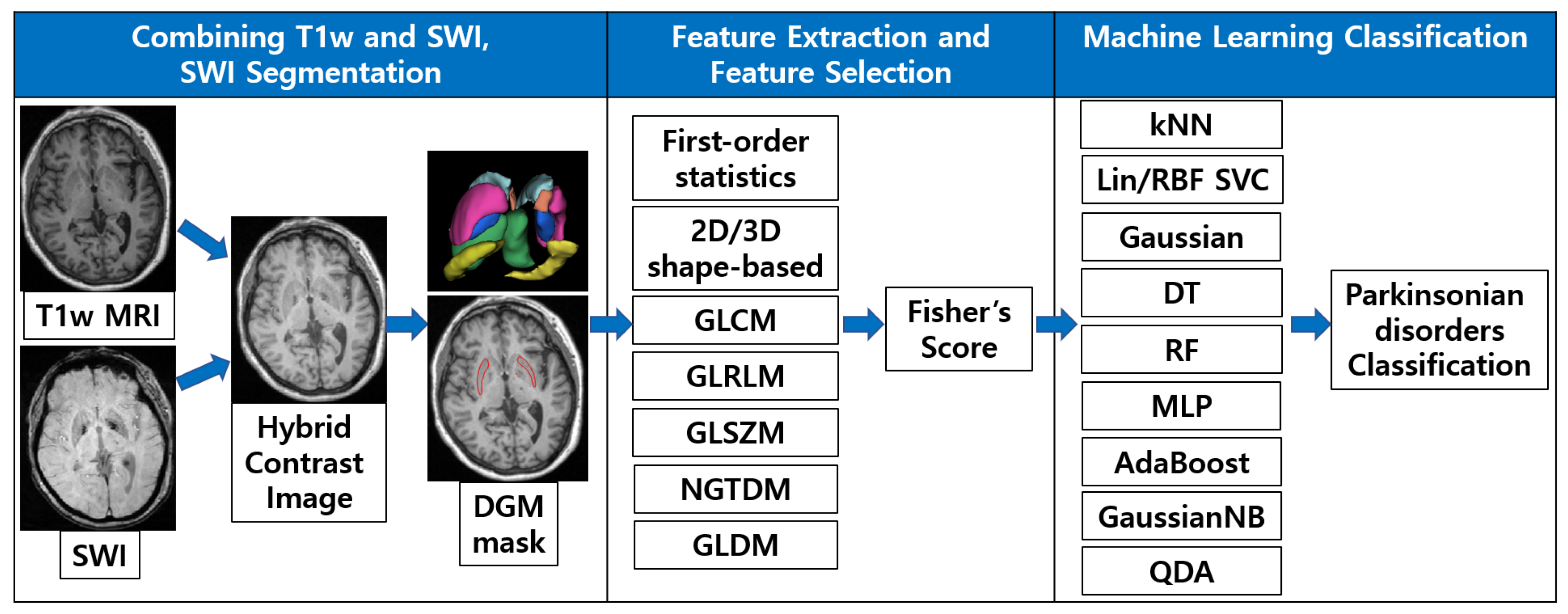
- We proposed a fully automatic framework for the analysis of iron deposition patterns in SWI.
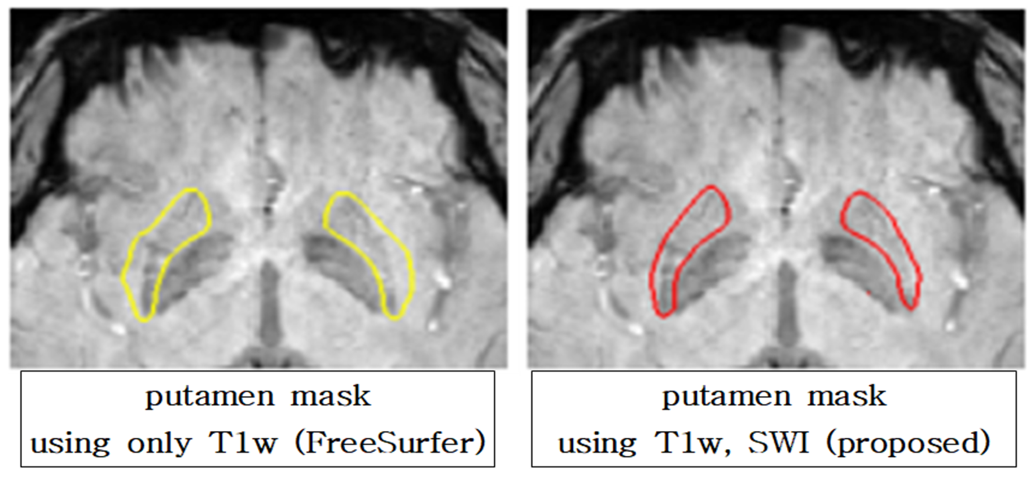
- We developed segmentation that reflects more the contrast of iron accumulation than conventional methods using a hybrid contrast image, which is created by image processing and combining T1w and SWI.
- We designed machine learning classifiers trained using texture-representing features extracted by our segmentation method.
- We demonstrated the improved performance of the machine learning classifier for differentiating APS using our segmentation framework.
2. Materials and Methods
2.1. Patients
2.2. Imaging Acquisition
2.3. Data Preprocessing and SWI Registration
2.4. SWI Segmentation Using Hybrid Contrast Image
2.5. Feature Extraction and Selection
2.6. Machine Learning Classifier Training and Testing
3. Results
3.1. Demographic Characteristics
3.2. SWI Segmentation Results
3.3. Feature Extraction and Selection Results
3.4. SVM Results
4. Discussion and Conclusions
Author Contributions
Funding
Institutional Review Board Statement
Informed Consent Statement
Data Availability Statement
Conflicts of Interest
Appendix A


Appendix B
Appendix B.1

| HC Features | MSA-P | MSA-C | T1w-Only Features | MSA-P | MSA-C |
|---|---|---|---|---|---|
| glszm_GrayLevelVariance | 6.8645 | 4.0758 | glcm_Id4 | 0.4473 | 0.5428 |
| glszm_HighGrayLevel- ZoneEmphasis | 70.981 | 40.6072 | glcm_ClusterTendency7 | 8.4945 | 3.201 |
| ngtdm_Strength | 0.2515 | 0.0898 | ngtdm_Strength | 0.2409 | 0.085 |
| ngtdm_Strength4 | 0.1409 | 0.0534 | gldm_SmallDependenceEmphasis | 0.0638 | 0.0331 |
| ngtdm_Strength7 | 0.1223 | 0.0495 | gldm_SmallDependence- LowGrayLevelEmphasis | 0.0021 | 0.0016 |
| glrlm_ShortRunHigh- GrayLevelEmphasis | 51.2291 | 24.4967 | glcm_ClusterShade | −61.4694 | −7.7083 |
| glcm_Imc24 | 0.5442 | 0.3803 | glcm_SumSquares4 | 6.3807 | 1.9578 |
| glcm_JointAverage7 | 8.1353 | 5.728 | glcm_Idm4 | 0.3788 | 0.4915 |
| glcm_SumAverage7 | 16.2706 | 11.4561 | glcm_ClusterShade4 | −12.6393 | −2.0909 |
| glszm_SmallAreaHigh- GrayLevelEmphasis | 34.8355 | 18.1394 | gldm_DependenceVariance | 23.2205 | 27.458 |
Appendix B.2
| HC Features | MSA-P | PD | T1w-Only Features | MSA-P | PD |
|---|---|---|---|---|---|
| glszm_ZoneVariance | 10,415.4 | 16,002.22 | ngtdm_Busyness4 | 6.2355 | 13.1834 |
| ngtdm_Busyness | 3.2868 | 6.393 | glcm_DifferenceAverage7 | 2.6958 | 1.9655 |
| glcm_JointAverage4 | 7.762 | 5.2133 | gldm_GrayLevelNonUniformity | 556.3621 | 736.7501 |
| glcm_ClusterShade4 | −11.6021 | −0.0316 | gldm_LargeDependence- HighGrayLevelEmphasis | 7484.096 | 3824.813 |
| gldm_SmallDependence- LowGrayLevelEmphasis | 0.0027 | 0.0028 | ngtdm_Strength | 0.2409 | 0.1118 |
| gldm_GrayLevelNonUniformity | 438.2295 | 550.6763 | gldm_HighGrayLevelEmphasis | 75.7005 | 38.6685 |
| gldm_DependenceNonUniformity | 186.9766 | 175.5947 | glcm_Idn4 | 0.8595 | 0.8683 |
| glcm_Imc14 | −0.074 | −0.0451 | glcm_DifferenceVariance4 | 4.8392 | 2.0783 |
| glcm_MCC4 | 0.3823 | 0.2921 | glrlm_GrayLevelNonUniformity | 344.9109 | 470.024 |
| glcm_Autocorrelation4 | 63.6349 | 28.8556 | glszm_HighGrayLevel- ZoneEmphasis | 75.1588 | 47.8979 |
Appendix B.3
| HC Features | MSA-C | PD | T1w-Only Features | MSA-C | PD |
|---|---|---|---|---|---|
| glcm_ClusterShade | −7.7694 | −1.3529 | glcm_ClusterShade4 | −2.0909 | 0.5222 |
| glcm_ClusterShade4 | −2.4839 | −0.4058 | glcm_ClusterShade | −7.7083 | −0.0626 |
| glcm_MCC4 | 0.2742 | 0.2319 | glcm_MCC4 | 0.3167 | 0.2744 |
| glcm_Imc14 | −0.0384 | −0.0291 | glcm_JointAverage7 | 5.8946 | 5.5243 |
| glcm_Imc24 | 0.3803 | 0.3244 | glcm_ClusterShade7 | −1.1194 | −0.1304 |
| glrlm_RunEntropy | 3.8955 | 3.7793 | gldm_DependenceVariance | 27.458 | 27.8954 |
| glcm_ClusterShade7 | −1.1463 | −0.3319 | glcm_Imc24 | 0.422 | 0.364 |
| gldm_DependenceEntropy | 6.499 | 6.3396 | glcm_Imc1 | −0.2039 | −0.1892 |
| glrlm_GrayLevelNon- UniformityNormalized | 0.2082 | 0.2397 | gldm_DependenceEntropy | 6.6475 | 6.518 |
| glcm_SumEntropy | 3.1802 | 2.9418 | glcm_MCC | 0.6602 | 0.6362 |
Appendix B.4
| HC Features | MSA-P | PD | T1w-Only Features | MSA-P | PD |
|---|---|---|---|---|---|
| glcm_MCC | 0.6103 | 0.6006 | gldm_DependenceVariance | 27.458 | 21.3893 |
| glrlm_RunEntropy | 3.8955 | 3.8289 | gldm_DependenceNon- UniformityNormalized | 0.0555 | 0.0642 |
| glcm_JointAverage7 | 5.728 | 5.4607 | ngtdm_Coarseness | 0.0024 | 0.0028 |
| glcm_Imc24 | 0.3803 | 0.4196 | glrlm_RunEntropy | 4.0075 | 4.0395 |
| glcm_MCC4 | 0.2742 | 0.2921 | glszm_LargeAreaHigh- GrayLevelEmphasis | 1,495,719 | 946,080.3 |
| gldm_LargeDependence- LowGrayLevelEmphasis | 6.085 | 6.0346 | glszm_LargeAreaLow- GrayLevelEmphasis | 1948.349 | 1398.383 |
| gldm_DependenceNonUniformity | 195.5685 | 175.5947 | glszm_LowGrayLevelZoneEmphasis | 0.0673 | 0.0777 |
| glszm_ZoneVariance | 31,931.73 | 16,002.22 | gldm_LargeDependenceEmphasis | 138.6942 | 109.827 |
| glszm_SmallAreaLow- GrayLevelEmphasis | 0.0275 | 0.0305 | gldm_GrayLevelVariance | 2.1446 | 2.9733 |
| glszm_ZoneEntropy | 5.0788 | 5.0619 | gldm_SmallDependence- LowGrayLevelEmphasis | 0.0016 | 0.002 |
Appendix B.5
| HC Features | MSA-P | PD | T1w-Only Features | MSA-P | PD |
|---|---|---|---|---|---|
| glcm_Autocorrelation7 | 27.9998 | 31.5698 | glcm_SumEntropy4 | 2.7913 | 3.1555 |
| glcm_Contrast7 | 2.7699 | 4.5716 | glcm_SumAverage7 | 11.0487 | 11.8343 |
| gldm_LargeDependenceHigh- GrayLevelEmphasis | 3796.027 | 2722.489 | gldm_HighGrayLevelEmphasis | 32.9521 | 38.6685 |
| glrlm_RunEntropy | 3.7793 | 3.8289 | gldm_LargeDependence- HighGrayLevelEmphasis | 4652.988 | 3824.813 |
| glcm_DifferenceAverage4 | 1.1238 | 1.4629 | gldm_LowGrayLevelEmphasis | 0.0474 | 0.0488 |
| gldm_DependenceVariance | 27.5647 | 19.9317 | glszm_ZonePercentage | 0.0192 | 0.0266 |
| glcm_ClusterProminence4 | 29.37 | 74.0809 | glcm_JointEnergy4 | 0.0702 | 0.0402 |
| glcm_JointAverage4 | 5.0443 | 5.2133 | glcm_ClusterShade | -0.0626 | 0.2446 |
| glcm_Imc24 | 0.3244 | 0.4196 | glcm_DifferenceEntropy4 | 2.007 | 2.306 |
| glrlm_RunPercentage | 0.6247 | 0.6961 | glszm_SizeZoneNonUniformity | 17.0448 | 19.3692 |
Appendix C
Appendix C.1
| Differentiating Diseases | Train | Test | ||
|---|---|---|---|---|
| HC | T1w-Only | HC | T1w-Only | |
| MSA-P vs. MSA-C | 0.8589 | 0.7677 | 0.8621 | 0.7910 |
| MSA-P vs. PD | 0.8839 | 0.8203 | 0.8865 | 0.8340 |
| MSA-P vs. PSP | 0.8357 | 0.8356 | 0.8569 | 0.8272 |
| MSA-C vs. PD | 0.6870 | 0.6613 | 0.6805 | 0.6613 |
| MSA-C vs. PSP | 0.7908 | 0.7855 | 0.7932 | 0.7813 |
| PD vs. PSP | 0.8895 | 0.7323 | 0.8761 | 0.8369 |
| Differentiating Diseases | Train | Test | ||||||||||
|---|---|---|---|---|---|---|---|---|---|---|---|---|
| HC | T1w-Only | HC | T1w-Only | |||||||||
| bAcc | Sen | Spe | bAcc | Sen | Spe | bAcc | Sen | Spe | bAcc | Sen | Spe | |
| MSA-P vs. MSA-C | 0.7915 | 0.8581 | 0.7250 | 0.6843 | 0.7889 | 0.5797 | 0.7906 | 0.8542 | 0.7269 | 0.7108 | 0.8054 | 0.6161 |
| MSA-P vs. PD | 0.8775 | 0.8682 | 0.8868 | 0.8057 | 0.7711 | 0.8402 | 0.8569 | 0.8259 | 0.8879 | 0.7924 | 0.7226 | 0.8622 |
| MSA-P vs. PSP | 0.7791 | 0.8574 | 0.7009 | 0.7712 | 0.8403 | 0.7020 | 0.8101 | 0.8803 | 0.7399 | 0.7867 | 0.8860 | 0.6874 |
| MSA-C vs. PD | 0.6513 | 0.4944 | 0.8082 | 0.6604 | 0.5292 | 0.7915 | 0.6779 | 0.5617 | 0.7949 | 0.6347 | 0.4776 | 0.7918 |
| MSA-C vs. PSP | 0.7196 | 0.7360 | 0.7032 | 0.6741 | 0.7237 | 0.6246 | 0.7242 | 0.7380 | 0.7103 | 0.6973 | 0.7305 | 0.6642 |
| PD vs. PSP | 0.8315 | 0.9033 | 0.7597 | 0.6147 | 0.8178 | 0.4116 | 0.8094 | 0.8981 | 0.7207 | 0.7330 | 0.8731 | 0.5928 |
| Differentiating Diseases | Train | Test | ||
|---|---|---|---|---|
| HC | T1w-Only | HC | T1w-Only | |
| MSA-P vs. MSA-C | 0.7955 | 0.6970 | 0.8006 | 0.7333 |
| MSA-P vs. PD | 0.8789 | 0.8163 | 0.8642 | 0.8095 |
| MSA-P vs. PSP | 0.8055 | 0.7929 | 0.8277 | 0.8123 |
| MSA-C vs. PD | 0.7387 | 0.7379 | 0.7420 | 0.722 |
| MSA-C vs. PSP | 0.7070 | 0.6644 | 0.7167 | 0.7016 |
| PD vs. PSP | 0.8667 | 0.7324 | 0.8569 | 0.8116 |
Appendix C.2
| Differentiating Diseases | Train | Test | ||
|---|---|---|---|---|
| HC | T1w-Only | HC | T1w-Only | |
| MSA-P vs. MSA-C | 0.8809 | 0.8790 | 0.8703 | 0.8631 |
| MSA-P vs. PD | 0.9159 | 0.8902 | 0.9156 | 0.8799 |
| MSA-P vs. PSP | 0.8840 | 0.8882 | 0.8928 | 0.8821 |
| MSA-C vs. PD | 0.7314 | 0.7097 | 0.7408 | 0.7261 |
| MSA-C vs. PSP | 0.9694 | 0.9349 | 0.9381 | 0.9300 |
| PD vs. PSP | 0.9433 | 0.8232 | 0.9346 | 0.8294 |
| Differentiating Diseases | Train | Test | ||||||||||
|---|---|---|---|---|---|---|---|---|---|---|---|---|
| HC | T1w-Only | HC | T1w-Only | |||||||||
| bAcc | Sen | Spe | bAcc | Sen | Spe | bAcc | Sen | Spe | bAcc | Sen | Spe | |
| MSA-P vs. MSA-C | 0.7995 | 0.8693 | 0.7297 | 0.7540 | 0.8907 | 0.6173 | 0.7832 | 0.8562 | 0.7102 | 0.7700 | 0.8962 | 0.6437 |
| MSA-P vs. PD | 0.8998 | 0.9178 | 0.8818 | 0.8593 | 0.8524 | 0.8662 | 0.8964 | 0.9075 | 0.8854 | 0.8495 | 0.8383 | 0.8607 |
| MSA-P vs. PSP | 0.7720 | 0.8705 | 0.6735 | 0.7459 | 0.8376 | 0.6542 | 0.7904 | 0.8824 | 0.6983 | 0.7733 | 0.8834 | 0.6633 |
| MSA-C vs. PD | 0.7830 | 0.7737 | 0.7923 | 0.7899 | 0.8111 | 0.7687 | 0.8212 | 0.8753 | 0.7670 | 0.7854 | 0.8026 | 0.7682 |
| MSA-C vs. PSP | 0.9038 | 0.8987 | 0.9089 | 0.8210 | 0.8166 | 0.8254 | 0.8573 | 0.8552 | 0.8594 | 0.8500 | 0.8355 | 0.8645 |
| PD vs. PSP | 0.8291 | 0.9108 | 0.7475 | 0.6747 | 0.8329 | 0.5166 | 0.8314 | 0.9140 | 0.7489 | 0.7377 | 0.8481 | 0.6272 |
| Differentiating Diseases | Train | Test | ||
|---|---|---|---|---|
| HC | T1w-Only | HC | T1w-Only | |
| MSA-P vs. MSA-C | 0.8052 | 0.7890 | 0.7921 | 0.7738 |
| MSA-P vs. PD | 0.8926 | 0.8619 | 0.8892 | 0.8392 |
| MSA-P vs. PSP | 0.8002 | 0.7732 | 0.8161 | 0.8019 |
| MSA-C vs. PD | 0.7883 | 0.7697 | 0.7691 | 0.7670 |
| MSA-C vs. PSP | 0.8907 | 0.8125 | 0.8419 | 0.8340 |
| PD vs. PSP | 0.8638 | 0.7781 | 0.8742 | 0.8127 |
Appendix C.3
| Differentiating Diseases | Train | Test | ||
|---|---|---|---|---|
| HC | T1w-Only | HC | T1w-Only | |
| MSA-P vs. MSA-C | 0.7420 | 0.6935 | 0.8529 | 0.6632 |
| MSA-P vs. PD | 0.9243 | 0.8753 | 0.9141 | 0.8790 |
| MSA-P vs. PSP | 0.8880 | 0.8277 | 0.8936 | 0.8735 |
| MSA-C vs. PD | 0.7018 | 0.6893 | 0.7185 | 0.6957 |
| MSA-C vs. PSP | 0.7354 | 0.7274 | 0.7574 | 0.7322 |
| PD vs. PSP | 0.6305 | 0.5029 | 0.5221 | 0.5000 |
| Differentiating Diseases | Train | Test | ||||||||||
|---|---|---|---|---|---|---|---|---|---|---|---|---|
| HC | T1w-Only | HC | T1w-Only | |||||||||
| bAcc | Sen | Spe | bAcc | Sen | Spe | bAcc | Sen | Spe | bAcc | Sen | Spe | |
| MSA-P vs. MSA-C | 0.7357 | 0.7826 | 0.6887 | 0.6948 | 0.7990 | 0.5905 | 0.7868 | 0.8738 | 0.6998 | 0.7388 | 0.8015 | 0.6762 |
| MSA-P vs. PD | 0.8916 | 0.8982 | 0.8849 | 0.8449 | 0.8238 | 0.8661 | 0.9024 | 0.9097 | 0.8951 | 0.8800 | 0.8958 | 0.8642 |
| MSA-P vs. PSP | 0.7412 | 0.8423 | 0.6401 | 0.7171 | 0.8159 | 0.6182 | 0.7590 | 0.8596 | 0.6584 | 0.7393 | 0.8532 | 0.6253 |
| MSA-C vs. PD | 0.7858 | 0.7922 | 0.7794 | 0.7781 | 0.7555 | 0.8006 | 0.7993 | 0.818 | 0.7806 | 0.7824 | 0.7836 | 0.7812 |
| MSA-C vs. PSP | 0.6655 | 0.7110 | 0.6201 | 0.6098 | 0.5594 | 0.6603 | 0.7171 | 0.7104 | 0.7238 | 0.6076 | 0.5661 | 0.6491 |
| PD vs. PSP | 0.7260 | 0.7909 | 0.6611 | 0.5803 | 0.8032 | 0.3574 | 0.7718 | 0.8081 | 0.7355 | 0.7699 | 0.7990 | 0.7408 |
| Differentiating Diseases | Train | Test | ||
|---|---|---|---|---|
| HC | T1w-Only | HC | T1w-Only | |
| MSA-P vs. MSA-C | 0.7515 | 0.7369 | 0.7933 | 0.7682 |
| MSA-P vs. PD | 0.8901 | 0.8530 | 0.8964 | 0.8571 |
| MSA-P vs. PSP | 0.7918 | 0.7690 | 0.8032 | 0.7884 |
| MSA-C vs. PD | 0.7929 | 0.78 | 0.7816 | 0.7770 |
| MSA-C vs. PSP | 0.6720 | 0.5594 | 0.7096 | 0.5661 |
| PD vs. PSP | 0.7857 | 0.7505 | 0.8033 | 0.8009 |
Appendix C.4
| Differentiating Diseases | Train | Test | ||
|---|---|---|---|---|
| HC | T1w-Only | HC | T1w-Only | |
| MSA-P vs. MSA-C | 0.8725 | 0.7894 | 0.8840 | 0.8504 |
| MSA-P vs. PD | 0.9135 | 0.8400 | 0.9078 | 0.8553 |
| MSA-P vs. PSP | 0.8462 | 0.8418 | 0.8632 | 0.8497 |
| MSA-C vs. PD | 0.7159 | 0.6951 | 0.7099 | 0.6649 |
| MSA-C vs. PSP | 0.9641 | 0.8880 | 0.9458 | 0.8152 |
| PD vs. PSP | 0.8896 | 0.8260 | 0.8869 | 0.8648 |
| Differentiating Diseases | Train | Test | ||||||||||
|---|---|---|---|---|---|---|---|---|---|---|---|---|
| HC | T1w-Only | HC | T1w-Only | |||||||||
| bAcc | Sen | Spe | bAcc | Sen | Spe | bAcc | Sen | Spe | bAcc | Sen | Spe | |
| MSA-P vs. MSA-C | 0.8168 | 0.8737 | 0.7599 | 0.7366 | 0.8170 | 0.6561 | 0.8138 | 0.8863 | 0.7412 | 0.7826 | 0.8847 | 0.6804 |
| MSA-P vs. PD | 0.8879 | 0.8924 | 0.8833 | 0.8301 | 0.8088 | 0.8514 | 0.8924 | 0.9013 | 0.8835 | 0.8645 | 0.8573 | 0.8717 |
| MSA-P vs. PSP | 0.7734 | 0.8299 | 0.7169 | 0.7262 | 0.8144 | 0.6380 | 0.7781 | 0.8530 | 0.7032 | 0.7753 | 0.8529 | 0.6976 |
| MSA-C vs. PD | 0.7196 | 0.6327 | 0.8065 | 0.7101 | 0.6278 | 0.7924 | 0.7359 | 0.6821 | 0.7898 | 0.7192 | 0.6453 | 0.7932 |
| MSA-C vs. PSP | 0.8920 | 0.8921 | 0.8918 | 0.7960 | 0.8117 | 0.7803 | 0.8674 | 0.8612 | 0.8736 | 0.8192 | 0.8233 | 0.8152 |
| PD vs. PSP | 0.7798 | 0.8696 | 0.6901 | 0.6968 | 0.8322 | 0.5614 | 0.7822 | 0.8772 | 0.6872 | 0.7234 | 0.8523 | 0.5945 |
| Differentiating Diseases | Train | Test | ||
|---|---|---|---|---|
| HC | T1w-Only | HC | T1w-Only | |
| MSA-P vs. MSA-C | 0.826 | 0.7475 | 0.8212 | 0.7902 |
| MSA-P vs. PD | 0.8855 | 0.8363 | 0.8857 | 0.8571 |
| MSA-P vs. PSP | 0.7941 | 0.7643 | 0.7994 | 0.7987 |
| MSA-C vs. PD | 0.7762 | 0.7639 | 0.7691 | 0.7670 |
| MSA-C vs. PSP | 0.8884 | 0.7839 | 0.8517 | 0.8083 |
| PD vs. PSP | 0.8295 | 0.7762 | 0.8336 | 0.8051 |
Appendix C.5
| Differentiating Diseases | Train | Test | ||
|---|---|---|---|---|
| HC | T1w-Only | HC | T1w-Only | |
| MSA-P vs. MSA-C | 0.7789 | 0.6615 | 0.7528 | 0.7000 |
| MSA-P vs. PD | 0.8568 | 0.7556 | 0.8688 | 0.7521 |
| MSA-P vs. PSP | 0.7426 | 0.7495 | 0.7631 | 0.7577 |
| MSA-C vs. PD | 0.6427 | 0.6192 | 0.6465 | 0.6208 |
| MSA-C vs. PSP | 0.8734 | 0.7890 | 0.8412 | 0.8180 |
| PD vs. PSP | 0.7453 | 0.6802 | 0.7433 | 0.7119 |
| Differentiating Diseases | Train | Test | ||||||||||
|---|---|---|---|---|---|---|---|---|---|---|---|---|
| HC | T1w-Only | HC | T1w-Only | |||||||||
| bAcc | Sen | Spe | bAcc | Sen | Spe | bAcc | Sen | Spe | bAcc | Sen | Spe | |
| MSA-P vs. MSA-C | 0.7650 | 0.8261 | 0.7040 | 0.6463 | 0.7504 | 0.5423 | 0.7409 | 0.8213 | 0.6605 | 0.6976 | 0.7371 | 0.6581 |
| MSA-P vs. PD | 0.8510 | 0.8383 | 0.8637 | 0.7745 | 0.7153 | 0.8337 | 0.8439 | 0.8189 | 0.8689 | 0.7752 | 0.6838 | 0.8666 |
| MSA-P vs. PSP | 0.7487 | 0.8268 | 0.6706 | 0.7375 | 0.8244 | 0.6507 | 0.7317 | 0.8353 | 0.6280 | 0.7271 | 0.8210 | 0.6332 |
| MSA-C vs. PD | 0.6842 | 0.5587 | 0.8096 | 0.6366 | 0.4693 | 0.8039 | 0.6529 | 0.5105 | 0.7953 | 0.6483 | 0.5017 | 0.7948 |
| MSA-C vs. PSP | 0.8725 | 0.8911 | 0.8539 | 0.7911 | 0.8082 | 0.7741 | 0.8438 | 0.8618 | 0.8257 | 0.8316 | 0.8295 | 0.8336 |
| PD vs. PSP | 0.7743 | 0.8768 | 0.6718 | 0.6794 | 0.8506 | 0.5082 | 0.7390 | 0.8808 | 0.5971 | 0.6934 | 0.8588 | 0.5281 |
| Differentiating Diseases | Train | Test | ||
|---|---|---|---|---|
| HC | T1w-Only | HC | T1w-Only | |
| MSA-P vs. MSA-C | 0.7712 | 0.6859 | 0.7539 | 0.7132 |
| MSA-P vs. PD | 0.8528 | 0.7888 | 0.8517 | 0.8035 |
| MSA-P vs. PSP | 0.7714 | 0.7746 | 0.7574 | 0.7561 |
| MSA-C vs. PD | 0.7497 | 0.7247 | 0.7329 | 0.7141 |
| MSA-C vs. PSP | 0.8712 | 0.7757 | 0.8378 | 0.8267 |
| PD vs. PSP | 0.8295 | 0.7581 | 0.8116 | 0.7878 |
Appendix C.6
| Differentiating Diseases | Train | Test | ||
|---|---|---|---|---|
| HC | T1w-Only | HC | T1w-Only | |
| MSA-P vs. MSA-C | 0.8750 | 0.7818 | 0.8768 | 0.8620 |
| MSA-P vs. PD | 0.9029 | 0.8714 | 0.9157 | 0.8770 |
| MSA-P vs. PSP | 0.8924 | 0.8753 | 0.9072 | 0.9000 |
| MSA-C vs. PD | 0.8084 | 0.7798 | 0.7900 | 0.7841 |
| MSA-C vs. PSP | 0.7850 | 0.6870 | 0.7597 | 0.6539 |
| PD vs. PSP | 0.8564 | 0.8097 | 0.8145 | 0.7541 |
| Differentiating Diseases | Train | Test | ||||||||||
|---|---|---|---|---|---|---|---|---|---|---|---|---|
| HC | T1w-Only | HC | T1w-Only | |||||||||
| bAcc | Sen | Spe | bAcc | Sen | Spe | bAcc | Sen | Spe | bAcc | Sen | Spe | |
| MSA-P vs. MSA-C | 0.6173 | 0.7607 | 0.4738 | 0.5687 | 0.6483 | 0.4891 | 0.7645 | 0.8367 | 0.6922 | 0.7135 | 0.8134 | 0.6136 |
| MSA-P vs. PD | 0.8054 | 0.8361 | 0.7748 | 0.6748 | 0.7015 | 0.6481 | 0.8951 | 0.9073 | 0.8830 | 0.8800 | 0.8958 | 0.8642 |
| MSA-P vs. PSP | 0.6904 | 0.8071 | 0.5738 | 0.6786 | 0.8146 | 0.5426 | 0.6416 | 0.8138 | 0.4693 | 0.6128 | 0.8051 | 0.4205 |
| MSA-C vs. PD | 0.7680 | 0.7275 | 0.8084 | 0.7364 | 0.6929 | 0.7798 | 0.7707 | 0.7514 | 0.7900 | 0.7386 | 0.6932 | 0.7841 |
| MSA-C vs. PSP | 0.5938 | 0.6532 | 0.5343 | 0.5134 | 0.5657 | 0.4612 | 0.5476 | 0.6254 | 0.4698 | 0.5056 | 0.4102 | 0.6010 |
| PD vs. PSP | 0.6555 | 0.7990 | 0.5121 | 0.6426 | 0.7833 | 0.5019 | 0.6943 | 0.7969 | 0.5918 | 0.6826 | 0.8099 | 0.5552 |
| Differentiating Diseases | Train | Test | ||
|---|---|---|---|---|
| HC | T1w-Only | HC | T1w-Only | |
| MSA-P vs. MSA-C | 0.7021 | 0.6444 | 0.7812 | 0.7575 |
| MSA-P vs. PD | 0.8153 | 0.7072 | 0.8875 | 0.8571 |
| MSA-P vs. PSP | 0.7886 | 0.7740 | 0.7890 | 0.7748 |
| MSA-C vs. PD | 0.7956 | 0.7685 | 0.7829 | 0.7725 |
| MSA-C vs. PSP | 0.6643 | 0.5643 | 0.6493 | 0.5172 |
| PD vs. PSP | 0.7705 | 0.7562 | 0.7551 | 0.7502 |
Appendix C.7
| Differentiating Diseases | Train | Test | ||
|---|---|---|---|---|
| HC | T1w-Only | HC | T1w-Only | |
| MSA-P vs. MSA-C | 0.8470 | 0.7486 | 0.8487 | 0.8287 |
| MSA-P vs. PD | 0.9079 | 0.8164 | 0.9021 | 0.8328 |
| MSA-P vs. PSP | 0.8697 | 0.8534 | 0.8426 | 0.8417 |
| MSA-C vs. PD | 0.7000 | 0.6536 | 0.6999 | 0.6743 |
| MSA-C vs. PSP | 0.9508 | 0.8884 | 0.9281 | 0.8939 |
| PD vs. PSP | 0.8789 | 0.7960 | 0.8806 | 0.8538 |
| Differentiating Diseases | Train | Test | ||||||||||
|---|---|---|---|---|---|---|---|---|---|---|---|---|
| HC | T1w-Only | HC | T1w-Only | |||||||||
| bAcc | Sen | Spe | bAcc | Sen | Spe | bAcc | Sen | Spe | bAcc | Sen | Spe | |
| MSA-P vs. MSA-C | 0.7619 | 0.8150 | 0.7088 | 0.6497 | 0.7368 | 0.5626 | 0.7486 | 0.8155 | 0.6816 | 0.7431 | 0.8158 | 0.6705 |
| MSA-P vs. PD | 0.8467 | 0.8163 | 0.8771 | 0.7562 | 0.6793 | 0.8330 | 0.8390 | 0.7969 | 0.8811 | 0.7770 | 0.7254 | 0.8286 |
| MSA-P vs. PSP | 0.7742 | 0.8378 | 0.7105 | 0.7450 | 0.8252 | 0.6648 | 0.7442 | 0.8369 | 0.6514 | 0.7275 | 0.8311 | 0.6239 |
| MSA-C vs. PD | 0.6421 | 0.4887 | 0.7956 | 0.6340 | 0.4683 | 0.7997 | 0.6632 | 0.5359 | 0.7906 | 0.6255 | 0.4586 | 0.7924 |
| MSA-C vs. PSP | 0.8725 | 0.8733 | 0.8716 | 0.8176 | 0.8336 | 0.8015 | 0.8656 | 0.8792 | 0.8521 | 0.8189 | 0.8321 | 0.8057 |
| PD vs. PSP | 0.7710 | 0.8879 | 0.6542 | 0.6861 | 0.8432 | 0.5290 | 0.7481 | 0.8743 | 0.6218 | 0.7143 | 0.8648 | 0.5638 |
| Differentiating Diseases | Train | Test | ||
|---|---|---|---|---|
| HC | T1w-Only | HC | T1w-Only | |
| MSA-P vs. MSA-C | 0.77 | 0.6896 | 0.7529 | 0.7563 |
| MSA-P vs. PD | 0.8535 | 0.7760 | 0.85 | 0.7976 |
| MSA-P vs. PSP | 0.7960 | 0.7728 | 0.7690 | 0.7587 |
| MSA-C vs. PD | 0.7262 | 0.7254 | 0.7279 | 0.7145 |
| MSA-C vs. PSP | 0.8696 | 0.8062 | 0.8588 | 0.8094 |
| PD vs. PSP | 0.8333 | 0.7733 | 0.8176 | 0.8036 |
Appendix C.8
| Differentiating Diseases | Train | Test | ||
|---|---|---|---|---|
| HC | T1w-Only | HC | T1w-Only | |
| MSA-P vs. MSA-C | 0.8915 | 0.8397 | 0.8849 | 0.8683 |
| MSA-P vs. PD | 0.9279 | 0.8787 | 0.9245 | 0.8817 |
| MSA-P vs. PSP | 0.9054 | 0.8765 | 0.8961 | 0.8777 |
| MSA-C vs. PD | 0.7088 | 0.6610 | 0.7120 | 0.6652 |
| MSA-C vs. PSP | 0.9658 | 0.8840 | 0.9493 | 0.8721 |
| PD vs. PSP | 0.9198 | 0.8600 | 0.9154 | 0.8657 |
| Differentiating Diseases | Train | Test | ||||||||||
|---|---|---|---|---|---|---|---|---|---|---|---|---|
| HC | T1w-Only | HC | T1w-Only | |||||||||
| bAcc | Sen | Spe | bAcc | Sen | Spe | bAcc | Sen | Spe | bAcc | Sen | Spe | |
| MSA-P vs. MSA-C | 0.8417 | 0.9317 | 0.7517 | 0.7596 | 0.8622 | 0.6571 | 0.8225 | 0.9231 | 0.7218 | 0.8138 | 0.9066 | 0.7210 |
| MSA-P vs. PD | 0.8938 | 0.8860 | 0.9016 | 0.8434 | 0.7991 | 0.8876 | 0.8922 | 0.8713 | 0.9132 | 0.8073 | 0.7518 | 0.8629 |
| MSA-P vs. PSP | 0.7722 | 0.8789 | 0.6656 | 0.7670 | 0.9023 | 0.6317 | 0.7867 | 0.8889 | 0.6845 | 0.7626 | 0.8838 | 0.6413 |
| MSA-C vs. PD | 0.6767 | 0.5359 | 0.8175 | 0.6600 | 0.5099 | 0.8100 | 0.7179 | 0.6320 | 0.8039 | 0.6850 | 0.5569 | 0.8132 |
| MSA-C vs. PSP | 0.8806 | 0.9005 | 0.8607 | 0.7567 | 0.7839 | 0.7295 | 0.8383 | 0.8792 | 0.7974 | 0.7493 | 0.7840 | 0.7146 |
| PD vs. PSP | 0.7566 | 0.9218 | 0.5913 | 0.7179 | 0.8922 | 0.5435 | 0.7515 | 0.9353 | 0.5676 | 0.7083 | 0.9123 | 0.5042 |
| Differentiating Diseases | Train | Test | ||
|---|---|---|---|---|
| HC | T1w-Only | HC | T1w-Only | |
| MSA-P vs. MSA-C | 0.8465 | 0.7705 | 0.8308 | 0.8272 |
| MSA-P vs. PD | 0.8948 | 0.8557 | 0.8964 | 0.8125 |
| MSA-P vs. PSP | 0.8030 | 0.7988 | 0.8135 | 0.7890 |
| MSA-C vs. PD | 0.7579 | 0.7322 | 0.7691 | 0.7562 |
| MSA-C vs. PSP | 0.8774 | 0.7556 | 0.8362 | 0.7581 |
| PD vs. PSP | 0.8162 | 0.7857 | 0.8133 | 0.7807 |
Appendix C.9
| Differentiating Diseases | Train | Test | ||
|---|---|---|---|---|
| HC | T1w-Only | HC | T1w-Only | |
| MSA-P vs. MSA-C | 0.8953 | 0.8550 | 0.9029 | 0.8749 |
| MSA-P vs. PD | 0.9317 | 0.8898 | 0.9200 | 0.9000 |
| MSA-P vs. PSP | 0.8915 | 0.8929 | 0.9150 | 0.9091 |
| MSA-C vs. PD | 0.6925 | 0.6929 | 0.7457 | 0.6580 |
| MSA-C vs. PSP | 0.9368 | 0.8589 | 0.9056 | 0.8382 |
| PD vs. PSP | 0.8870 | 0.7944 | 0.8951 | 0.8638 |
| Differentiating Diseases | Train | Test | ||||||||||
|---|---|---|---|---|---|---|---|---|---|---|---|---|
| HC | T1w-Only | HC | T1w-Only | |||||||||
| bAcc | Sen | Spe | bAcc | Sen | Spe | bAcc | Sen | Spe | bAcc | Sen | Spe | |
| MSA-P vs. MSA-C | 0.7903 | 0.8005 | 0.7801 | 0.6847 | 0.7916 | 0.5778 | 0.8179 | 0.8595 | 0.7762 | 0.7937 | 0.8567 | 0.7307 |
| MSA-P vs. PD | 0.8818 | 0.8510 | 0.9126 | 0.8445 | 0.8005 | 0.8885 | 0.8804 | 0.8501 | 0.9107 | 0.8273 | 0.7688 | 0.8858 |
| MSA-P vs. PSP | 0.7996 | 0.7916 | 0.8076 | 0.7877 | 0.7975 | 0.7779 | 0.8381 | 0.8561 | 0.8201 | 0.8199 | 0.8655 | 0.7742 |
| MSA-C vs. PD | 0.7051 | 0.5971 | 0.8130 | 0.6555 | 0.5179 | 0.7932 | 0.7204 | 0.6295 | 0.8112 | 0.6669 | 0.5567 | 0.7772 |
| MSA-C vs. PSP | 0.8885 | 0.8281 | 0.9489 | 0.7630 | 0.7646 | 0.7614 | 0.7948 | 0.7871 | 0.8025 | 0.7655 | 0.7607 | 0.7704 |
| PD vs. PSP | 0.7868 | 0.8655 | 0.7081 | 0.7213 | 0.8434 | 0.5991 | 0.7841 | 0.8926 | 0.6755 | 0.7414 | 0.8892 | 0.5937 |
| Differentiating Diseases | Train | Test | ||
|---|---|---|---|---|
| HC | T1w-Only | HC | T1w-Only | |
| MSA-P vs. MSA-C | 0.7921 | 0.7478 | 0.8266 | 0.8111 |
| MSA-P vs. PD | 0.8880 | 0.8564 | 0.8857 | 0.8392 |
| MSA-P vs. PSP | 0.7944 | 0.7816 | 0.8445 | 0.8374 |
| MSA-C vs. PD | 0.7706 | 0.7362 | 0.7741 | 0.7341 |
| MSA-C vs. PSP | 0.8479 | 0.7287 | 0.7812 | 0.7478 |
| PD vs. PSP | 0.8314 | 0.7933 | 0.8407 | 0.8180 |
References
- Barbagallo, G.; Sierra-Peña, M.; Nemmi, F.; Traon, A.P.L.; Meissner, W.G.; Rascol, O.; Péran, P. Multimodal MRI assessment of nigro-striatal pathway in multiple system atrophy and Parkinson disease. Mov. Disord. 2016, 31, 142–149. [Google Scholar] [CrossRef] [PubMed]
- Jellinger, K.A. Neuropathological spectrum of synucleinopathies. Mov. Disord. 2003, 18, 2–12. [Google Scholar] [CrossRef] [PubMed]
- Ward, R.J.; Zucca, F.A.; Duyn, J.H.; Crichton, R.R.; Zecca, L. The role of iron in brain ageing and neurodegenerative disorders. Lancet Neurol. 2014, 13, 1045–1060. [Google Scholar] [CrossRef] [Green Version]
- Kaindlstorfer, C.; Jellinger, K.A.; Eschlböck, S.; Stefanova, N.; Weiss, G.; Wenning, G.K. The relevance of iron in the pathogenesis of multiple system atrophy: A viewpoint. J. Alzheimer’s Dis. 2018, 61, 1253–1273. [Google Scholar] [CrossRef] [Green Version]
- Peeraully, T. Multiple system atrophy. Semin. Neurol. 2014, 34, 290–292. [Google Scholar] [CrossRef] [PubMed]
- Wang, N.; Edmiston, E.K.; Luo, X.; Yang, H.; Chang, M.; Wang, F.; Fan, G. Comparing abnormalities of amplitude of low-frequency fluctuations in multiple system atrophy and idiopathic Parkinson’s disease measured with resting-state fMRI. Psychiatry Res. Neuroimaging 2017, 269, 73–81. [Google Scholar] [CrossRef]
- Hikishima, K.; Ando, K.; Yano, R.; Kawai, K.; Komaki, Y.; Inoue, T.; Itoh, T.; Yamada, M.; Momoshima, S.; Okano, H.J.; et al. Parkinson disease: Diffusion MR imaging to detect nigrostriatal pathway loss in a marmoset model treated with 1-methyl-4-phenyl-1,2,3,6-tetrahydropyridine. Radiology 2015, 275, 430–437. [Google Scholar] [CrossRef]
- Pang, H.; Yu, Z.; Li, R.; Yang, H.; Fan, G. MRI-based radiomics of basal nuclei in differentiating idiopathic Parkinson’s disease From parkinsonian variants of multiple system atrophy: A susceptibility-weighted imaging study. Front. Aging Neurosci. 2020, 12, 587250. [Google Scholar] [CrossRef]
- Saeed, U.; Lang, A.E.; Masellis, M. Neuroimaging Advances in Parkinson’s Disease and Atypical Parkinsonian Syndromes. Front. Neurol. 2020, 11, 572976. [Google Scholar] [CrossRef]
- Aludin, S.; Schmill, L.A. MRI Signs of Parkinson’s Disease and Atypical Parkinsonism. Rofo 2021, 193, 1403–1410. [Google Scholar]
- Sodickson, A.; Baeyens, P.F.; Andriole, K.P.; Prevedello, L.M.; Nawfel, R.D.; Hanson, R.; Khorasani, R. Recurrent CT, cumulative radiation exposure, and associated radiation-induced cancer risks from CT of adults. Radiology 2009, 251, 175–184. [Google Scholar] [CrossRef] [PubMed]
- Alster, P.; Nieciecki, M.; Migda, B.; Kutyłowski, M.; Madetko, N.; Duszyńska-Wąs, K.; Charzyńska, I.; Koziorowski, D.; Królicki, L.; Friedman, A. The Strengths and Obstacles in the Differential Diagnosis of Progressive Supranuclear Palsy—Parkinsonism Predominant (PSP-P) and Multiple System Atrophy (MSA) Using Magnetic Resonance Imaging (MRI) and Perfusion Single Photon Emission Computed Tomography (SPECT). Diagnostics 2022, 12, 385. [Google Scholar] [PubMed]
- Lee, J.H.; Baik, S.K. Putaminal hypointensity in the parkinsonian variant of multiple system atrophy: Simple visual assessment using susceptibility-weighted imaging. J. Mov. Disord. 2011, 4, 60–63. [Google Scholar] [CrossRef] [PubMed]
- Lee, J.H.; Lee, M.S. Brain iron accumulation in atypical parkinsonian syndromes: In vivo MRI evidences for distinctive patterns. Front. Neurol. 2019, 10, 74. [Google Scholar] [CrossRef] [Green Version]
- Gupta, D.; Saini, J.; Kesavadas, C.; Sarma, P.S.; Kishore, A. Utility of susceptibility-weighted MRI in differentiating Parkinson’s disease and atypical parkinsonism. Neuroradiology 2010, 52, 1087–1094. [Google Scholar] [CrossRef]
- Harder, S.L.; Hopp, K.M.; Ward, H.; Neglio, H.; Gitlin, J.; Kido, D. Mineralization of the deep gray matter with age: A retrospective review with susceptibility-weighted MR imaging. Am. J. Neuroradiol. 2008, 29, 176–183. [Google Scholar] [CrossRef] [Green Version]
- Cheng, Z.; Zhang, J.; He, N.; Li, Y.; Wen, Y.; Xu, H.; Tang, R.; Jin, Z.; Haacke, E.M.; Yan, F.; et al. Radiomic features of the nigrosome-1 region of the substantia nigra: Using quantitative susceptibility mapping to assist the diagnosis of idiopathic Parkinson’s disease. Front. Aging Neurosci. 2019, 11, 167. [Google Scholar] [CrossRef] [Green Version]
- Fischl, B.; Salat, D.H.; Busa, E.; Albert, M.; Dieterich, M.; Haselgrove, C.; van der Kouwe, A.; Killiany, R.; Kennedy, D.; Klaveness, S.; et al. Whole brain segmentation: Automated labeling of neuroanatomical structures in the human brain. Neuron 2002, 33, 341–355. [Google Scholar] [CrossRef] [Green Version]
- Fischl, B. FreeSurfer. NeuroImage 2012, 62, 774–781. [Google Scholar] [CrossRef] [Green Version]
- Patenaude, B.; Smith, S.M.; Kennedy, D.N.; Jenkinson, M. A Bayesian model of shape and appearance for subcortical brain segmentation. Neuroimage 2011, 56, 907–922. [Google Scholar] [CrossRef] [Green Version]
- Wang, J.; Vachet, C.; Rumple, A.; Gouttard, S.; Ouziel, C.; Perrot, E.; Du, G.; Huang, X.; Gerig, G.; Styner, M. Multi-atlas segmentation of subcortical brain structures via the AutoSeg software pipeline. Front. Neuroinform. 2014, 8, 7. [Google Scholar] [CrossRef] [PubMed] [Green Version]
- Morey, R.A.; Selgrade, E.S.; Wagner, H.R., 2nd; Huettel, S.A.; Wang, L.; McCarthy, G. Scan-rescan reliability of subcortical brain volumes derived from automated segmentation. Hum. Brain Mapp. 2010, 31, 1751–1762. [Google Scholar] [PubMed] [Green Version]
- Nugent, A.C.; Luckenbaugh, D.A.; Wood, S.E.; Bogers, W.; Zarate, C.A., Jr.; Drevets, W.C. Automated subcortical segmentation using FIRST: Test-retest reliability, interscanner reliability, and comparison to manual segmentation. Hum. Brain Mapp. 2013, 34, 2313–2329. [Google Scholar] [CrossRef] [PubMed] [Green Version]
- de Sitter, A.; Verhoeven, T.; Burggraaff, J.; Liu, Y.; Simoes, J.; Ruggieri, S.; Palotai, M.; Brouwer, I.; Versteeg, A.; Wottschel, V.; et al. Reduced accuracy of MRI deep grey matter segmentation in multiple sclerosis: An evaluation of four automated methods against manual reference segmentations in a multi-center cohort. J. Neurol. 2020, 267, 3541–3554. [Google Scholar] [CrossRef] [PubMed]
- Derakhshan, M.; Caramanos, Z.; Giacomini, P.S.; Narayanan, S.; Maranzano, J.; Francis, S.J.; Arnold, D.L.; Collins, D.L. Evaluation of automated techniques for the quantification of grey matter atrophy in patients with multiple sclerosis. Neuroimage 2010, 52, 1261–1267. [Google Scholar] [CrossRef]
- Litvan, I.; Agid, Y.; Calne, D.; Campbell, G.; Dubois, B.; Duvoisin, R.C. Clinical research criteria for the diagnosis of progressive supranuclear palsy (Steel-Richardson-Olszewski syndrome): Report of the NINDSSPSP international workshop. Neurology 1996, 47, 1–9. [Google Scholar] [CrossRef]
- Gilman, S.; Wenning, G.K.; Low, P.A.; Brooks, D.J.; Mathias, C.J.; Trojanowski, J.Q.; Wood, N.W.; Colosimo, C.; Dürr, A.; Fowler, C.J.; et al. Second consensus statement on the diagnosis of multiple system atrophy. Neurology 2008, 71, 670–676. [Google Scholar] [CrossRef]
- Hughes, A.J.; Daniel, S.E.; Kilford, L.; Lees, A.J. Accuracy of clinical diagnosis of idiopathic Parkinson’s disease: A clinico-pathological study of 100 cases. J. Neurol. Neurosurg. Psychiatry 1992, 55, 181–184. [Google Scholar] [CrossRef] [Green Version]
- Tustison, N.J.; Avants, B.B.; Cook, P.A.; Zheng, Y.; Egan, A.; Yushkevich, P.A.; Gee, J.C. N4ITK: Improved N3 bias correction. IEEE Trans. Med. Imaging 2010, 29, 1310–1320. [Google Scholar] [CrossRef] [Green Version]
- Feng, X.; Deistung, A.; Dwyer, M.G.; Hagemeier, J.; Polak, P.; Lebenberg, J.; Frouin, F.; Zivadinov, R.; Reichenbach, J.R.; Schweser, F. An improved FSL-FIRST pipeline for subcortical gray matter segmentation to study abnormal brain anatomy using quantitative susceptibility mapping (QSM). Magn. Reason. Imaging 2017, 39, 110–122. [Google Scholar] [CrossRef]
- Jones, B.C.; Nair, G.; Shea, C.D.; Crainiceanu, C.M.; Cortese, I.C.; Reich, D.S. Quantification of multiple-sclerosis-related brain atrophy in two heterogeneous MRI datasets using mixed-effects modeling. Neuroimage Clin. 2013, 3, 171–179. [Google Scholar] [CrossRef] [PubMed] [Green Version]
- Avants, B.B.; Tustison, N.J.; Song, G.; Cook, P.A.; Klein, A.; Gee, J.C. A reproducible evaluation of ANTs similarity metric performance in brain image registration. Neuroimage 2011, 54, 2033–2044. [Google Scholar] [CrossRef] [PubMed] [Green Version]
- Klein, A.; Andersson, J.; Ardekani, B.A.; Ashburner, J.; Avants, B.; Chiang, M.C.; Christensen, G.E.; Collins, D.L.; Gee, J.; Hellier, P.; et al. Evaluation of 14 nonlinear deformation algorithms applied to human brain MRI registration. Neuroimage 2009, 46, 786–802. [Google Scholar] [CrossRef] [PubMed] [Green Version]
- Van Griethuysen, J.J.M.; Fedorov, A.; Parmar, C.; Hosny, A.; Aucoin, N.; Narayan, V.; Beets-Tan, R.G.H.; Fillion-Robin, J.C.; Pieper, S.; Aerts, H.J.W.L. Computational radiomics system to decode the radiographic phenotype. Cancer Res. 2017, 77, e104–e107. [Google Scholar] [CrossRef] [Green Version]
- Available online: https://pyradiomics.readthedocs.io/en/latest/index.html (accessed on 22 January 2022).
- Wu, Y.; Jiang, J.H.; Chen, L.; Lu, J.Y.; Ge, J.J.; Liu, F.T.; Yu, J.T.; Lin, W.; Zuo, C.T.; Wang, J. Use of radiomic features and support vector machine to distinguish Parkinson’s disease cases from normal controls. Ann. Transl. Med. 2019, 7, 773. [Google Scholar] [CrossRef]
- Salmanpour, M.R.; Shamsaei, M.; Rahmim, A. Feature selection and machine learning methods for optimal identification and prediction of subtypes in Parkinson’s disease. Comput. Methods Programs Biomed. 2021, 206, 106131. [Google Scholar] [CrossRef]
- Suguna, N.; Thanushkodi, K. An improved k-nearest neighbor classification using genetic algorithm. Int. J. Comput. Sci. Issues 2010, 7, 18–21. [Google Scholar]
- Chang, C.C.; Lin, C.J. LIBSVM: A library for support vector machines. ACM Trans. Intell. Syst. Technol. 2011, 2, 1–27. [Google Scholar] [CrossRef]
- Kuo, B.C.; Ho, H.H.; Li, C.H.; Hung, C.C. A kernel-based feature selection method for SVM with RBF kernel for hyperspectral image classification. IEEE J. Sel. Top. Appl. Earth Obs. Remote Sens. 2013, 7, 317–326. [Google Scholar] [CrossRef]
- Rasmussen, C.E. Gaussian processes for machine learning. In Summer School on Machine Learning; Springer: Berlin/Heidelberg, Germany, 2003; pp. 63–71. [Google Scholar]
- Ali, J.; Khan, R.; Ahmad, N.; Maqsood, I. Random forests and decision trees. Int. J. Comput. Sci. Issues 2012, 9, 272–278. [Google Scholar]
- Chourasia, S. Survey paper on improved methods of ID3 decision tree classification. Int. J. Sci. Res. Publ. 2013, 3, 1–4. [Google Scholar]
- He, K.; Zhang, X.; Ren, S.; Sun, J. Delving deep into rectifiers: Surpassing human-level performance on imagenet classification. In Proceedings of the IEEE International Conference on Computer Vision, Santiago, Chile, 7–13 December 2015; pp. 1026–1034. [Google Scholar]
- Hastie, T.; Rosset, S.; Zhu, J.; Zuo, H. Multi-class adaboost. Stat. Its Interface 2009, 2, 349–360. [Google Scholar] [CrossRef] [Green Version]
- Chan, T.F.; Golub, G.H.; LeVeque, R.J. Updating formulae and a pairwise algorithm for computing sample variances. In COMPSTAT 1982 5th Symposium Held at Toulouse 1982; Physica: Heidelberg, Germany, 1982; pp. 30–41. [Google Scholar]
- Srivastava, M.R.; Gupta, M.R.; Frigyik, B.A. Bayesian quadratic discriminant analysis. J. Mach. Learn. Res. 2007, 8, 1277–1305. [Google Scholar]
- Feng, Q.; Chen, Y.; Liao, Z.; Jiang, H.; Mao, D.; Wang, M. Corpus callosum radiomics-based classification model in alzheimer’s disease: A case-control study. Front. Neurol. 2018, 9, 618. [Google Scholar] [CrossRef] [PubMed] [Green Version]
- Zwanenburg, A.; Leger, S.; Vallieres, M.; Lock, S. Image biomarker standardisation initiative. arXiv 2016, arXiv:1612.07003. [Google Scholar]
- Lee, M.J.; Kim, T.H.; Kim, S.J.; Kim, B.K.; Mun, C.W.; Lee, J.H. Quantitative Validation of a Visual Rating Scale for Defining High-Iron Putamen in Patients with Multiple System Atrophy. Front. Neurol. 2019, 10, 1014. [Google Scholar] [CrossRef] [Green Version]


| Neuroimaging Modality | Role of Modality | Potential of Differentiating PD and APS |
|---|---|---|
| Diffusion-tensor image (DTI) [7] | Detect characteristics such as fractional anisotropy (FA) and mean diffusion (MD) | Decreased FA and/or increased MD in the substantia nigra, the corpus callosum, the frontal lobes, the cingulum, and the temporal cortex |
| Positron emission tomography (PET) [9] | Measure amyloid pathology, tau pathology, a-Synuclein pathology, metabolic activity by measuring changes in the glucose consumption | PD-related spatial covariance pattern may involve increased pallidothalamic and pontine activity associated with decreased metabolism in supplementary motor area, premotor cortex, and parietal association areas |
| Single photon emission computed tomography (SPECT) [12] | Measure dopamine transporter (DAT) density, dopamine D2 receptor, metabolic activity by measuring changes in the cerebral blood flow | Decreased striatal presynaptic DAT binding contralateral to parkinsonian symptomatology with greater reduction in posterior putamen than in anterior putamen or caudate nucleus |
| Susceptibility weighted image (SWI) [13] | Visualize iron-related contents sensitively | Substantia nigra pars compacta, globus pallidus internus, the putamen, and the red nucleus have been described as regions with increased iron concentration |
| MSA-P | MSA-C | PSP | PD | Significance | |
|---|---|---|---|---|---|
| Gender (M/F) | 13/21 | 9/12 | 11/6 | 32/24 | p = 0.179 (3) = 4.894 |
| Age (years) | 59.05 ± 7.83 | 58.95 ± 6.30 | 65.64 ± 5.58 | 56.85 ± 7.60 | p < 0.001 F(3,124) = 6.052 |
| UPDRS-III | 39.73 ± 12.86 | 30.80 ± 9.73 | 35.94 ± 8.15 | 24.33 ± 9.57 | p < 0.001 F(3,124) = 16.597 |
| H-Y stage | 3.10 ± 0.76 | 3.14 ± 0.61 | 3.5 ± 0.75 | 2.02 ± 0.51 | p < 0.001 F(3,124) = 36.885 |
| Duration (months) | 30.23 ± 15.25 | 30.52 ± 13.62 | 31.11 ± 18.09 | 35.41 ± 22.23 | p = 0.661 F(3,124) = 0.532 |
| MMSE | 25.44 ± 2.73 | 24.76 ± 3.23 | 23.82 ± 4.03 | 26.89 ± 2.41 | p < 0.001 F(3,124) = 6.395 |
| Features by HC | MSA-P | PD | Features by T1w-Only | MSA-P | PD |
|---|---|---|---|---|---|
| glrlm_ShortRunHigh- GrayLevelEmphasis | 51.2291 | 20.3952 | glcm_MCC4 | 0.4166 | 0.2744 |
| glcm_Autocorrelation7 | 69.2407 | 27.9998 | glcm_Imc24 | 0.5665 | 0.364 |
| glcm_JointAverage7 | 8.1353 | 5.1994 | glcm_JointAverage7 | 8.4094 | 5.5243 |
| glcm_SumAverage7 | 16.2706 | 10.3988 | glcm_SumAverage7 | 16.8187 | 11.0487 |
| gldm_HighGrayLevelEmphasis | 64.9219 | 27.8777 | gldm_DependenceVariance | 23.2205 | 27.8954 |
| glrlm_HighGrayLevelRunEmphasis | 64.0086 | 28.202 | glrlm_GrayLevelNonUniformity | 344.9109 | 652.5307 |
| glcm_Imc24 | 0.5442 | 0.3244 | glcm_Autocorrelation7 | 72.6811 | 31.5304 |
| glcm_Autocorrelation4 | 63.6349 | 26.3972 | glcm_SumAverage4 | 16.1899 | 10.7769 |
| glcm_SumAverage4 | 15.5239 | 10.0885 | glcm_JointAverage4 | 8.095 | 5.3884 |
| glcm_JointAverage4 | 7.762 | 5.0443 | gldm_HighGrayLevelEmphasis | 75.7005 | 32.9521 |
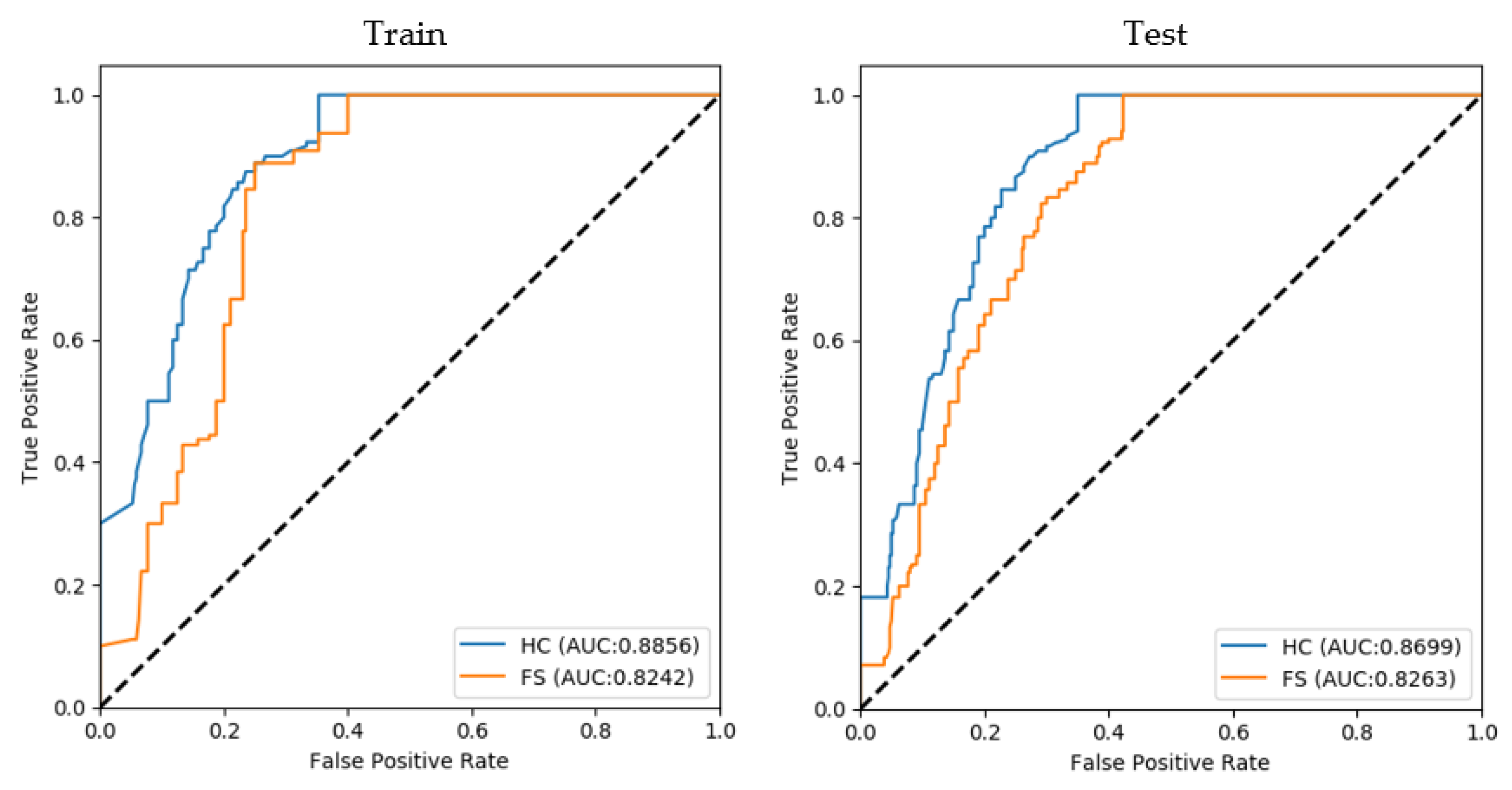
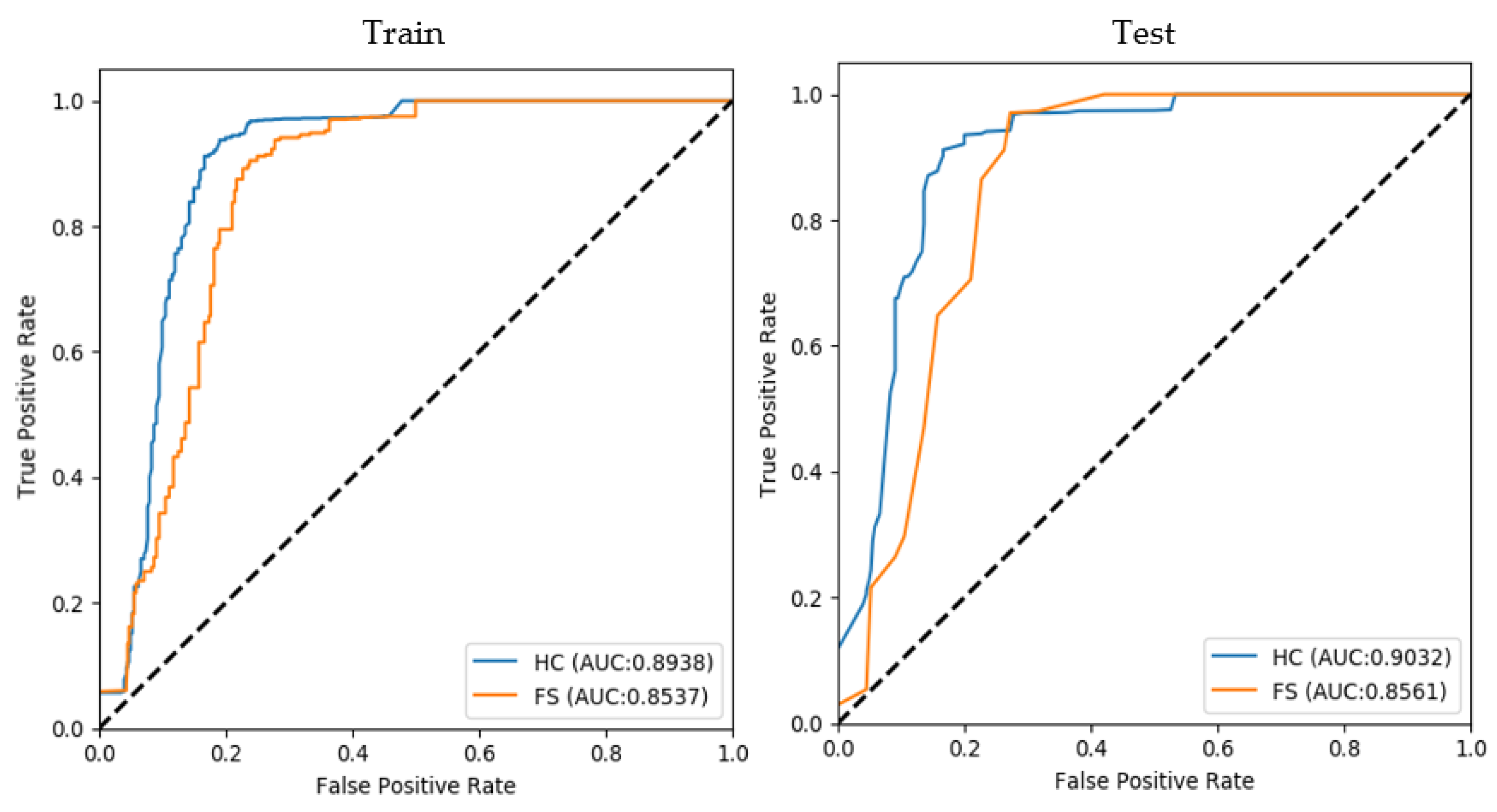
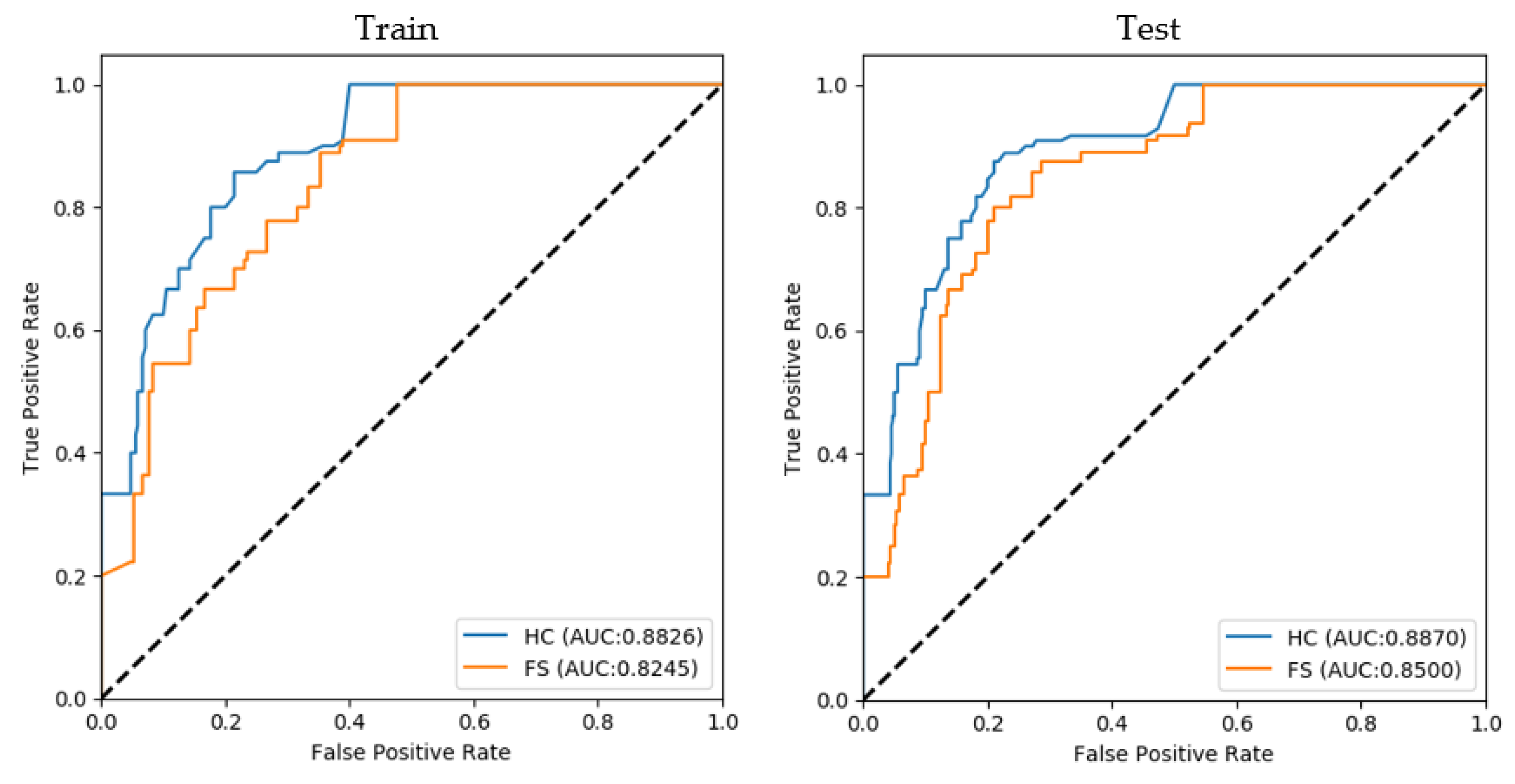
| Differentiating Diseases | Train AUC | Test AUC | ||
|---|---|---|---|---|
| HC | T1w-Only | HC | T1w-Only | |
| MSA-P vs. MSA-C | 0.8856 | 0.8242 | 0.8699 | 0.8263 |
| MSA-P vs. PD | 0.8938 | 0.8537 | 0.9032 | 0.8561 |
| MSA-P vs. PSP | 0.8825 | 0.8245 | 0.8869 | 0.8499 |
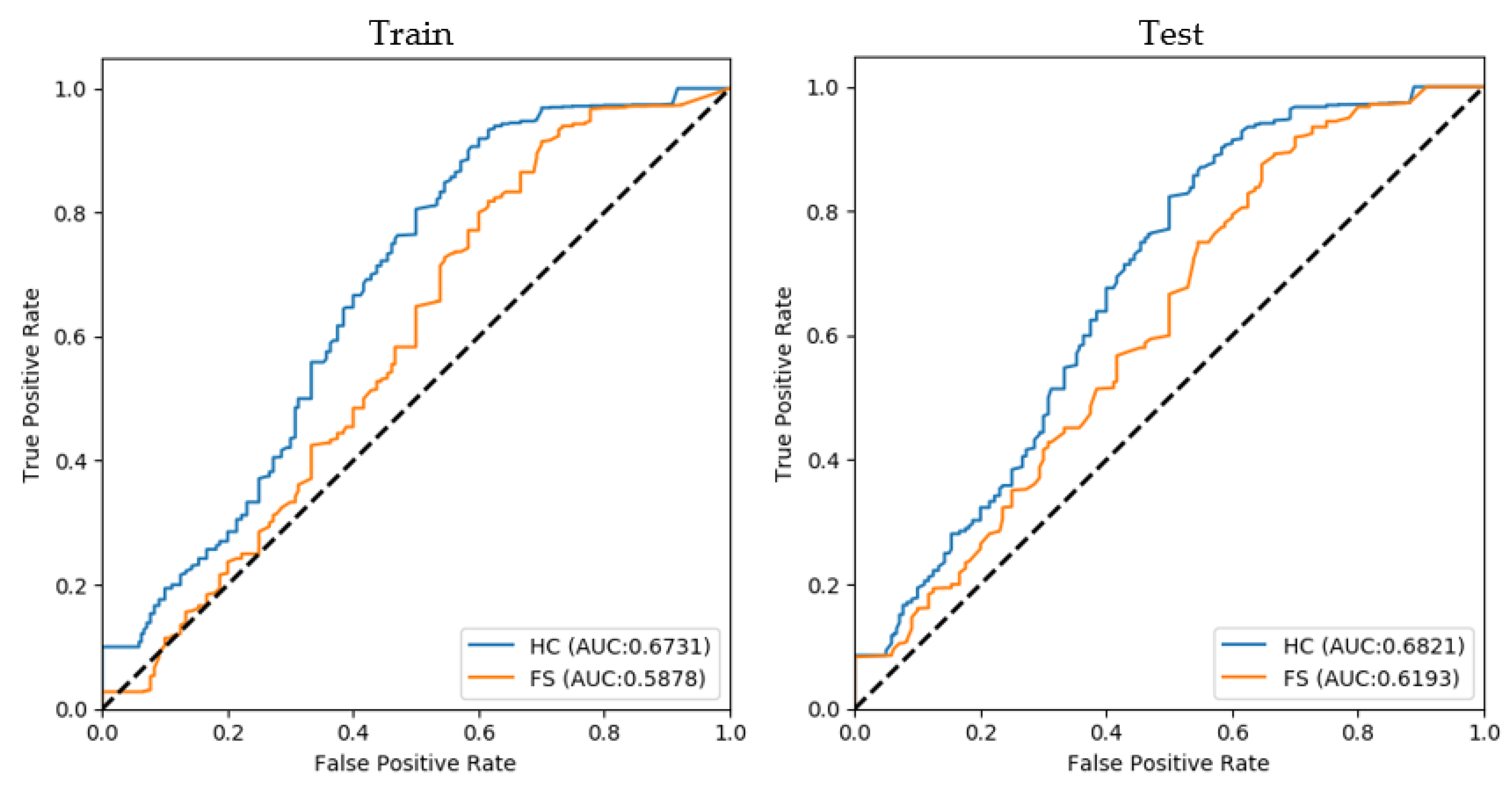
| MSA-C vs. PD | 0.6731 | 0.5878 | 0.6820 | 0.6193 |
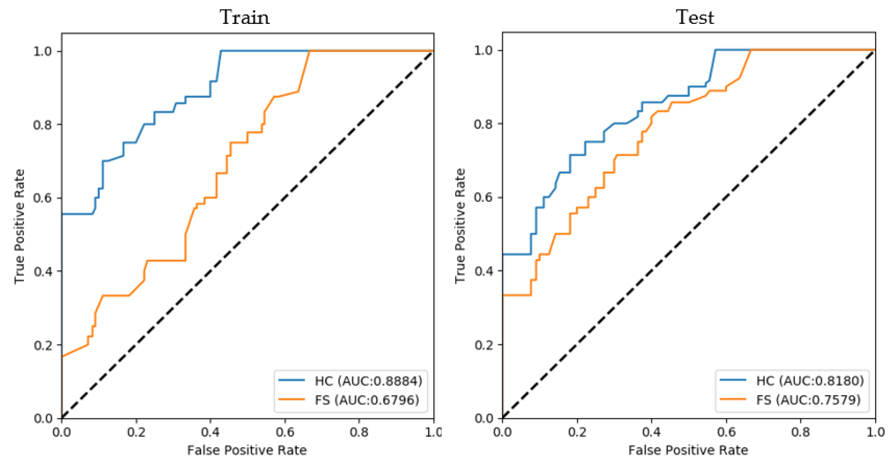
| MSA-C vs. PSP | 0.8883 | 0.6796 | 0.8180 | 0.7578 |
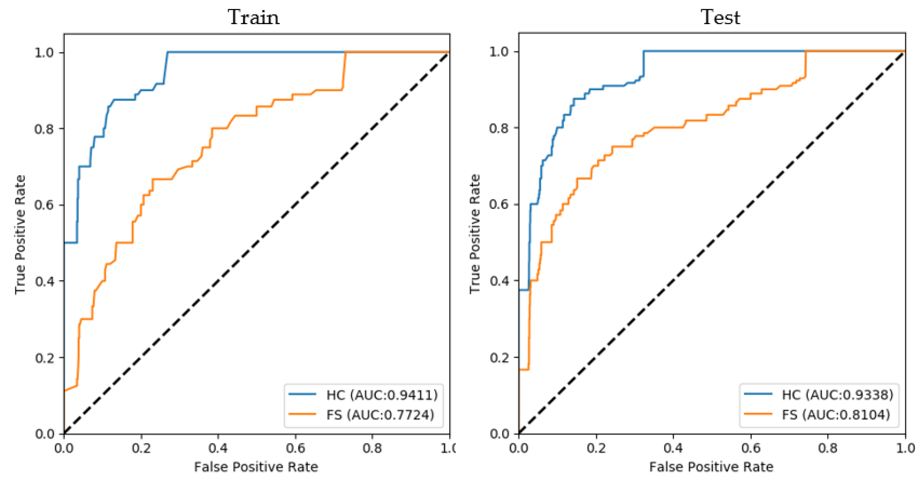
| PD vs. PSP | 0.9411 | 0.7724 | 0.9338 | 0.8104 |
| Differentiating Diseases | Train | Test | ||||||||||
|---|---|---|---|---|---|---|---|---|---|---|---|---|
| HC | T1w-Only | HC | T1w-Only | |||||||||
| bAcc | Sen | Spe | bAcc | Sen | Spe | bAcc | Sen | Spe | bAcc | Sen | Spe | |
| MSA-P vs. MSA-C | 0.7931 | 0.8472 | 0.7390 | 0.7005 | 0.8045 | 0.5963 | 0.7922 | 0.8662 | 0.7183 | 0.7313 | 0.8298 | 0.6327 |
| MSA-P vs. PD | 0.9120 | 0.8865 | 0.8937 | 0.8482 | 0.8316 | 0.8647 | 0.8981 | 0.9046 | 0.8917 | 0.8800 | 0.8958 | 0.8642 |
| MSA-P vs. PSP | 0.7790 | 0.8707 | 0.6874 | 0.6023 | 0.7854 | 0.4193 | 0.7862 | 0.8802 | 0.6922 | 0.7535 | 0.8345 | 0.6725 |
| MSA-C vs. PD | 0.7863 | 0.7727 | 0.7999 | 0.7516 | 0.7335 | 0.7698 | 0.7899 | 0.7988 | 0.7810 | 0.7872 | 0.8031 | 0.7714 |
| MSA-C vs. PSP | 0.7470 | 0.8045 | 0.6895 | 0.5491 | 0.6714 | 0.4269 | 0.7262 | 0.8020 | 0.6505 | 0.6828 | 0.6838 | 0.6818 |
| PD vs. PSP | 0.5823 | 0.7914 | 0.3732 | 0.4826 | 0.7757 | 0.1894 | 0.8027 | 0.8194 | 0.7860 | 0.7376 | 0.7807 | 0.0776 |
| Differentiating Diseases | Train ACC | Test ACC | ||
|---|---|---|---|---|
| HC | T1w-Only | HC | T1w-Only | |
| MSA-P vs. MSA-C | 0.7972 | 0.7336 | 0.8018 | 0.7552 |
| MSA-P vs. PD | 0.8944 | 0.8544 | 0.8928 | 0.8571 |
| MSA-P vs. PSP | 0.8087 | 0.6902 | 0.8135 | 0.7692 |
| MSA-C vs. PD | 0.7960 | 0.7682 | 0.7804 | 0.7708 |
| MSA-C vs. PSP | 0.7172 | 0.5973 | 0.7288 | 0.6616 |
| PD vs. PSP | 0.7867 | 0.7676 | 0.8184 | 0.778 |
Publisher’s Note: MDPI stays neutral with regard to jurisdictional claims in published maps and institutional affiliations. |
© 2022 by the authors. Licensee MDPI, Basel, Switzerland. This article is an open access article distributed under the terms and conditions of the Creative Commons Attribution (CC BY) license (https://creativecommons.org/licenses/by/4.0/).
Share and Cite
Kim, Y.S.; Lee, J.-H.; Gahm, J.K. Automated Differentiation of Atypical Parkinsonian Syndromes Using Brain Iron Patterns in Susceptibility Weighted Imaging. Diagnostics 2022, 12, 637. https://0-doi-org.brum.beds.ac.uk/10.3390/diagnostics12030637
Kim YS, Lee J-H, Gahm JK. Automated Differentiation of Atypical Parkinsonian Syndromes Using Brain Iron Patterns in Susceptibility Weighted Imaging. Diagnostics. 2022; 12(3):637. https://0-doi-org.brum.beds.ac.uk/10.3390/diagnostics12030637
Chicago/Turabian StyleKim, Yun Soo, Jae-Hyeok Lee, and Jin Kyu Gahm. 2022. "Automated Differentiation of Atypical Parkinsonian Syndromes Using Brain Iron Patterns in Susceptibility Weighted Imaging" Diagnostics 12, no. 3: 637. https://0-doi-org.brum.beds.ac.uk/10.3390/diagnostics12030637