Development of Hybrid Intelligent Models for Prediction Machining Performance Measure in End Milling of Ti6Al4V Alloy with PVD Coated Tool under Dry Cutting Conditions

Abstract

Ti6Al4V alloy is widely used in aerospace and medical applications. It is classified as a difficult to machine material due to its low thermal conductivity and high chemical reactivity. In this study, hybrid intelligent models have been developed to predict surface roughness when end milling Ti6Al4V alloy with a Physical Vapor Deposition PVD coated tool under dry cutting conditions. Back propagation neural network (BPNN) has been hybridized with two heuristic optimization techniques, namely: gravitational search algorithm (GSA) and genetic algorithm (GA). Taguchi method was used with an L27 orthogonal array to generate 27 experiment runs. Design expert software was used to do analysis of variances (ANOVA). The experimental data were divided randomly into three subsets for training, validation, and testing the developed hybrid intelligent model. ANOVA results revealed that feed rate is highly affected by the surface roughness followed by the depth of cut. One-way ANOVA, including a Post-Hoc test, was used to evaluate the performance of three developed models. The hybrid model of Artificial Neural Network-Gravitational Search Algorithm (ANN-GSA) has outperformed Artificial Neural Network (ANN) and Artificial Neural Network-Genetic Algorithm (ANN-GA) models. ANN-GSA achieved minimum testing mean square error of 7.41 × 10⁻¹³ and a maximum R-value of 1. Further, its convergence speed was faster than ANN-GA. GSA proved its ability to improve the performance of BPNN, which suffers from local minima problems.

1. Introduction

Ti alloy is an important superalloy that has many applications in the biomedical, aerospace, and chemical industries due to its properties and characteristics. Ti alloys have, therefore, a good market and demand for them is still increasing due to their unique properties [1]. Every year, many metals are transformed into chips during machining. Moreover, the issue becomes more crucial and critical for superalloys; because Ti-alloys are expensive and difficult to machine, they pose a big challenge for researchers and machinists. This is due to the high chemical reaction of Ti alloy with other materials and the low thermal conductivity.

Su et al. [2] investigated the performance of coated cemented carbide tools in high-speed end milling of Ti-6Al-4V under various cooling conditions like dry, flood coolant, nitrogen-oil-mist, compressed cold nitrogen gas (CCNG) at 0 °C and 100 °C, and compressed cold nitrogen gas and oil mist (CCNGOM). This study aimed to identify or determine the optimal cooling/lubrication condition for enhancing the tool life. The researchers observed flank wear as the most dominating mode of failure mode under all the cooling conditions.

Elmagrabi et al. [3] conducted a study in which they performed experimental tests on Ti-6Al-4V with coated and uncoated carbide cutting tools at a variety of cutting speeds of 50, 80, and 105 m/min, with a depth of cuts of 1, 1.5, and 2 mm, and feed rates of 0.1, 0.15, and 2 mm/tooth, respectively. They employed response surface methodology (RSM) in developing a statistical model for prediction of tool life and surface roughness. To determine the performance of the cutting tool, the researchers used both tool life and the quality of the surface finish. Based on the results, it was observed that the PVD-coated carbide tool was found to have a better tool life with a maximum of 11.5 min, and surface roughness showed more sensitivity to the feed rate and depth of cut.

Li et al. [4] commented that complicated wear mechanisms have been found when dry milling Ti6Al4V alloy with Chemical Vapor Deposition (CVD) coated carbide tools at a variety of high cutting speeds. Mechanical damage was observed at low cutting speed due to mechanical loading, while high cutting speed promotes thermal damage, which in turn creates main tool wear mechanisms. It was found that tool wear is a crucial variable that plays a key and deciding role.

Safari et al. [5] studied the effect of end milling conditions and tool wear on the surface integrity of Ti6Al4V alloy. New and used TiAlN + TiN PVD coated tools with different cutting speeds (100–300 m/min) and feed rates (0.03 and 0.06 mm/tooth) were utilized in carrying out the required experiments. It was found that surface roughness was highly affected by the tool condition at a higher cutting speed, where new tools achieved 185 nm in contrast with 320 nm for the used one. The high level of feed rate degraded the surface quality, particularly at low cutting speed, while high cutting speed produced plastic deformation in the sub-surface zone.

Ahmadi et al. [6] studied the effect of fine-equiaxed and enlarged equiaxed microstructures of Ti6Al4V alloys on cutting forces, build-up edge, and surface roughness during micro end milling. The microstructures of the milled surface were analyzed by electron backscatter diffraction (EBSD) technique. The authors observed that fine grain (each of α + β) with a small amount of β produced higher cutting forces. Also, the microstructure affected the formation of the build-up edge and corresponding size.

The effect of liquid nitrogen (LN2) on the surface integrity during milling Ti6Al4V alloy was investigated by Zhao et al. [7]. An improvement in the surface finish was noticed at a temperature range (20~−196), and high microhardness and compressive residual stresses were produced from using LN2 as a coolant. No noticeable variation was found for grain refinement compared to the dry milling process. The authors confirmed the usefulness of cryogenic milling in enhancing surface integrity.

Paese et al. [8] evaluated the performance of CVD, PVD, and cermet inserts after turning the AISI 1045 carbons steel shaft by using ANOVA analysis and response surface methodology. The cermet and PVD coated inserts generated minimum surface roughness compared with the CVD insert.

Danil [9] Analyzed the published works related to the machinability of titanium alloys and closed topics. They reviewed the performance of different coolants and lubricants such as traditional cooling conditions, dry cutting, cutting under minimum quantity cooling lubrication, subzero and cryogenic cutting conditions, applying the minimum quantity of lubricant to the cutting processes, and cooling with high-pressure coolants.

Creating a realistic model to predict machining performance measures will help to minimize machining time and costs. Based on previous research, there have been a vast number of techniques attempted and developed by many researchers as means of solving such kinds of parameter optimization problems, and such techniques can be categorized as traditional and non-traditional optimization techniques. For the recently well-known and extensively used non-conventional meta-heuristic search-based techniques, they are stated to be sufficiently general and based on genetic algorithm (GA), artificial neural networks (ANN), adaptive neuro-fuzzy inference system (ANFIS), tabu search (TS), particle swarm (PS), ant colony (AC), genetic programming (GP), and simulated annealing (SA) [10]. For example, neural networks can be applied in many fields and can replace large numerical simulations [11,12].

Öktem [13] developed an ANN model coupled with GA for optimizing cutting conditions and predicting surface roughness in end milling of AISI 1040 plain carbon steel. Multiple regression and ANOVA were also used to study the effect of cutting conditions on surface roughness. The proposed integrated method (GA with feed-forward BP neural networks) reduced the machining time to 20% with a 3.27% error.

Del Prete et al. [14] utilized RSM to develop a prediction model for surface roughness in flat-end mill operation. ANN was applied to estimate surface roughness; however, GA was applied to optimize the surface roughness model. Feed rate, depth of cut, radial engage, and speed were taken as the process parameters in this study. The developed RSM model was merged with a developed GA to find the optimal process parameters leading to the minimum surface roughness value. The estimated adequate process parameters were validated with experimental measurements showing that, depending on the different examined process parameters, GA enhanced the surface roughness with respect to non-optimized experimental tests from 13% to 27%. The developed RSM model merged with GA, and the optimization methodology proved effective mainly if the developed RSM model was accurate.

Bharathi and Baskar [15] applied particle swarm optimization to predict surface roughness while milling aluminium materials. An analytical model was established to predict surface roughness by using Particle Swarm Optimization (PSO) from the basis of these experimental results. The author discovered that the constraints associated with both the theoretical and the experimental approaches were similar to the actual roughness.

Zain et al. [16] suggested the implementation of ANN and GA techniques to the process parameter values (speed, feed, and radial rake angle) of end milling machining that result in a minimum value of surface roughness. According to the experimental results, the minimal surface roughness value achieved was 0.139 μm, and the optimal process parameters were speed = 167.029 m/min, feed = (0.025 mm/tooth), and radial rake angle = 4.769°. The authors affirmed that the surface roughness value achieved was much lower, about 26.8%, 25.7%, 26.1%, and 49.8%, compared to the experimental, regression, ANN, and RSM results, respectively. The experiments also diminished the mean surface roughness value and the number of iterations by about 0.61% and 23.9%, respectively, compared to the conventional GA results.

Moghri et al. [17] conducted a study in which they used a combination of experiments and an artificial intelligence approach to optimize surface roughness in milling polyamide-6 (PA-6) nanocomposites to develop a predictive model. The researchers developed a surface roughness ANN predictive model based on milling parameters (spindle speed and feed rate) and nano clay (NC) content using an artificial neural network (ANN). Since the data used in this study were the relatively small amount of data which was obtained from full factorial design, the researchers applied the genetic algorithm (GA) for ANN training since it suits the purpose of the study, which was to develop an accurate and robust ANN model. The optimization results showed that surface roughness in the milling of PA-6/NC nanocomposites is minimal at the lowest feed rate level and an intermediate spindle speed level.

A radial basis neural network model was developed by AL-Khafaji [18] to predict cutting forces and chip thickness ratio during the turning of AA 7020-T6 aluminum alloy. A good correlation was obtained between the input parameters represented by cutting speed, feed rate, depth of cut and cutting force, and chip thickness as output responses. The developed models also found the optimum conditions that minimize both cutting forces and chip thickness ratios at 240.46 N and 1.21.

The end milling of Inconel 690 alloy was carried out by Sen et al. [19] with assistance of the minimum quantity lubricants (MQL) of vegetable oil synergy. They applied different algorithms to model the achieved experimental data. The selected algorithms were gene expression programming (GEP) to produce the equation to enable the non-dominated sorting genetic algorithm to search for various solutions in order to permit the technique for order preference by similarity to the ideal solution model (TOPSIS) to pick up the best solution among non-dominated Pareto optimized solutions. The average error between experimental and predicted results was 3.31%.

Ibrahim [20] modeled the cutting forces produced during metal cutting of AISI 52100 by using an artificial neural network. Cutting speed, feed rate, and depth of cut values were fed into the neural network model to predict cutting, feed, and radial forces. Twenty-five experimental runs were divided into two subsets: 19 experiments for network training and 6 for testing the generalization of the developed neural model. The most significant factors affecting the generated forces were feed rate followed by the cut depth and good mapping produced between experimental and predicted values.

Rahimi et al. [21] integrated machine learning network with a physics-based model to estimate the amount of chatter during the milling process. The hybrid model reached 98% prediction accuracy of chatter and permitted extra training of the network with the assistance of a deterministic physical-based model during the production process.

Boga et al. [22] examined the influence of end milling parameters of carbon fiber composite material with high strength. Further, a combined neural network-genetic algorithm model was introduced to predict the achieved surface roughness. The findings analysis showed that surface finish was highly impacted by cutting tool and feed rate, whose optimized values were: coated tool with TiAlN, 250 mm/rev, and the cutting speed of 5000 rev/min. The hybrid model achieved a Mean Square Error (MSE) of 0.074.

Unfortunately, the backpropagation algorithm that was applied widely by several investigators suffers from sticking in local minima that impede reaching the global solution. In the last few years, numerous metaheuristic optimization algorithms have been developed to solve several complicated engineering issues, and they are mostly inspired by the work on natural and swarm conduct. The gravitational search algorithm is one of the metaheuristic optimization approaches that was firstly proposed by [23] to solve the optimization problem for combinatorial benchmark data. It works based on the laws of Newtonian and gravitational motion. Later, it was applied to solve various engineering problems; for example, Chatterjee et al. [24] integrated GSA with wavelet mutation (GSAWM) [25,26] and used it to solve the Economic Load Dispatch (ELD) problem taking into account the effect of valve-point. Mondal et al. [27] implemented the GSA for the IEEE 30-bus framework with six traditional thermal generators. Also, Duman et al. [28] adopted GSA to solve the IEEE 30-bus test system having six generators under various conditions using different fitness functions. The reactive power dispatch problem in multiple cases has been solved by applying GSA by Duman et al. [29]. The issue of the real-time energy management system has been solved by using GSA by Marzband et al. [30] in micro-grids involving various kinds of distributed generation units with particular precaution paid to the technical limits. The GSA was combined with the K-means method by Hatamlou et al. [31] to optimize the clustering problem. The classification problem is also solved by GSA Bahrololoum et al. [32]. The problem of the traveling salesman was also solved by GSA Dowlatshahi et al. [33].

The GSA was also implemented in the filter design and communication system, where Saha et al. [34] optimized the design of the IIR filter by integrating Wavelet Mutation with GSA. Competitive findings were achieved by Ji et al. [35] when they applied binary GSA to the wind power system for the unit commitment.

Based on what was stated above, the authors were motivated to contribute to the current study by developing a hybrid intelligence model via integrating the backpropagation neural network (BPNN) with a gravitational search algorithm to overcome the possibility of entrapping the BPNN with local minima. The study validated the capability of the gravitational search algorithm in optimizing the backpropagation neural network parameters to minimize the MSE between actual and desired targets. The details of the best model were illustrated in terms of its coefficients (weights and biases), unlike other studies that present the best structure of the ANN models.

Further, an extensive statistical evaluation was performed to prove the superiority of the developed ANN-GSA over other neural models by utilizing four statistical measures (MEAN, MEDIAN, Standard Deviation (STDV), and Best) and applying a post hoc test.

2. Experimental Work

The Ti6Al4V alloy was machined using a 5-Axis Milling Machine DMU 70 (DMG MORI Aktiengesellschaft, Bielefeld, Germany). It is a new model and had not been used yet in the GMI (German Malaysian Institute). It was selected to achieve accurate results because it is free from any vibrations and works in excellent condition. It has spindle speeds of up to 18,000 rpm and rapid traverses of 24 m/min.

The material that has been investigated in this study was Ti6Al4V alloy. It is an aerospace material and classified as difficult to machine.

Table 1. Mechanical properties of Ti6Al4V alloy [36].

Ultimate Tensile Strength MPa	Yield Strength MPa	Rockwell Hardness HRC	Modulus of Elasticity GPa	Poisson’s Ratio
950	880	36	113.8	0.342

shows the mechanical properties of Ti6Al4V alloy.

The cutting tool used in end milling Ti6Al4V alloy under dry cutting conditions is a PVD coated cutting tool.

Table 2. Cutting tools specifications.

Tool Type	Insert Cutting Rake Angle	Insert Side Clearance Angle	Insert Helix Angle	Insert Radius
1-ISO grade K20-(S20-S30)-XOMX090308TR ME06 (SECO Tools, SDN.BHD., Kuala Lumpur, Malaysia), F40 (PVD-Coated Carbide Ti-Al-N) with chamfer of 0.06 width at 4°	24°	11°	15°	8 mm

shows the specifications and geometrical dimensions of this cutting tool. The cutting inserts were mounted in a tool holder type R217.69-1612.0-09-1A with a diameter of 12 mm.

Generally, classical experimental design methods are too complex and not so easy to use. A large number of experiments have to be carried out when the number of process parameters increases. To solve this problem, the Taguchi method [37] used a special design of orthogonal arrays to successfully design and conduct fractional factorial experiments that can collect all the statistically significant data with a minimum possible number of repetitions.

Two-level and three-level orthogonal array structures are commonly used to accommodate the factor and level in the Taguchi method. A fractional factorial design was chosen in conducting 27 experimental runs and used a standard orthogonal array (L27 (313)). This array is selected based on its ability to investigate the interaction among parameters that affect the response.

Table 3. Factors levels.

	Levels	1	2	3
Factors
A-Cutting speed (m/min.)		50	77.5	105
B-Feed rate (mm/rev.)		0.1	0.15	0.2
C-Depth of cut (mm)		1	1.5	2

presents the cutting conditions: cutting speed (m/min), feed rate (mm/min), and depth of cut (mm). Each cutting condition was coded with low, medium, and high levels to disguise the problem domain and investigate its effect on surface roughness. The lower and upper limits of the cutting conditions are shown in Table 3. The radial depth of the cut was kept constant at 8 mm.

Table 4. Design matrix of L27 orthogonal array.

No.	Cutting Speed (m/min.)	Feed Rate (mm/Tooth)	Depth of Cut (mm)
1	50	0.1	1
2	50	0.15	1.5
3	50	0.2	2
4	77.5	0.1	1
5	77.5	0.15	1.5
6	77.5	0.2	2
7	105	0.1	1
8	105	0.15	1.5
9	105	0.2	2
10	50	0.1	1.5
11	50	0.15	2
12	50	0.2	1
13	77.5	0.1	1.5
14	77.5	0.15	2
15	77.5	0.2	1
16	105	0.1	1.5
17	105	0.15	2
18	105	0.2	1
19	50	0.1	2
20	50	0.15	1
21	50	0.2	1.5
22	77.5	0.1	2
23	77.5	0.15	1
24	77.5	0.2	1.5
25	105	0.1	2
26	105	0.15	1
27	105	0.2	1.5

shows the design matrix of the L 27 Taguchi orthogonal array. It consists of 27 runs with different cutting conditions but within the indicated range in Table 1.

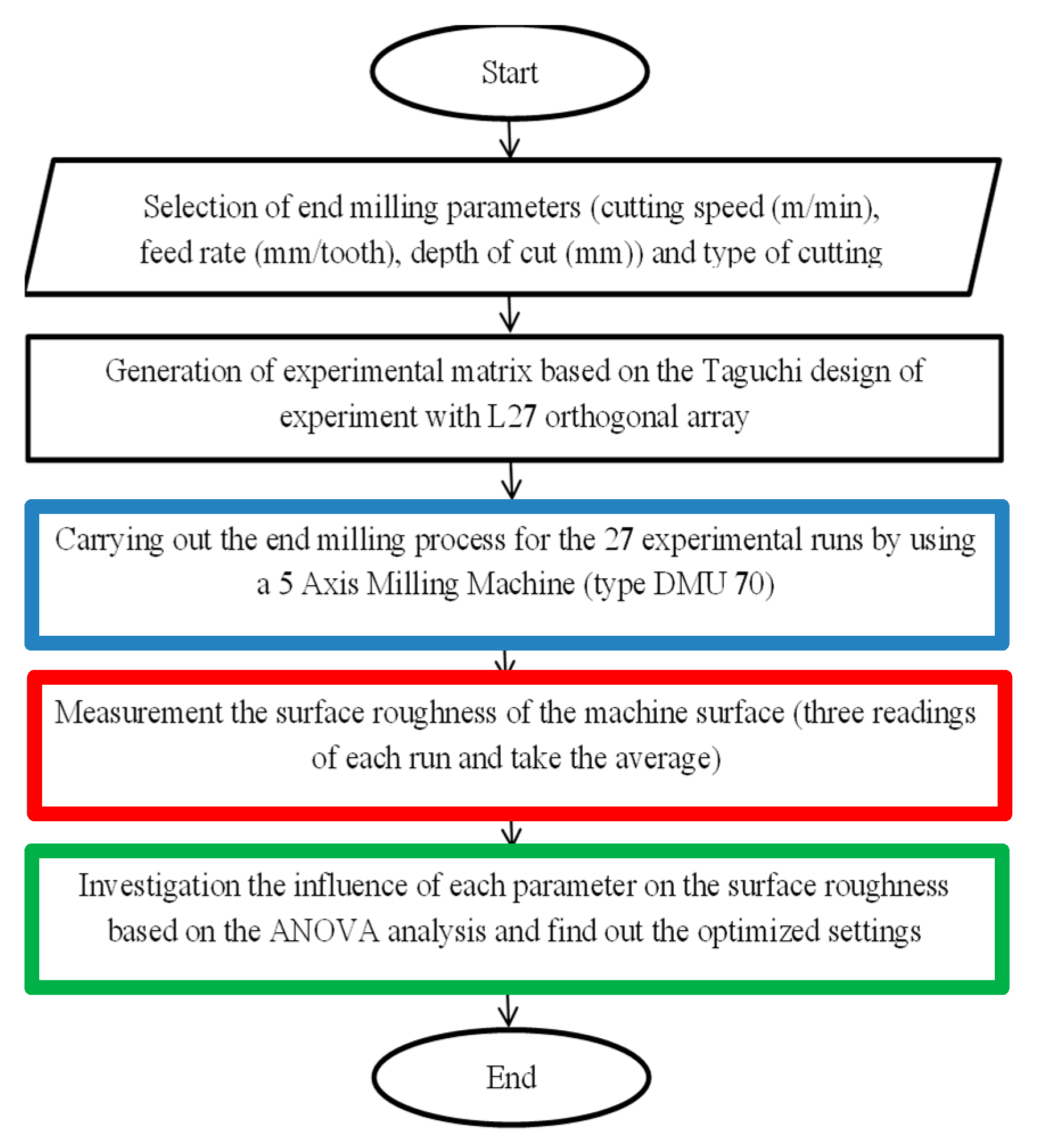
Ti6Al4V block with dimensions (166 × 105 × 30 mm³) was clamped tightly with vice and machined by using a pocketing process to remove dust and contaminations or residual stresses and prepare the block for experimental run. A G-code program was written, and after each pass, the surface roughness value Ra of the machined surface was measured in the direction parallel to feed motion by using a portable surface roughness tester (Mpi Mahr perthometer model, Mahr GMbH, Göttingen Germany). Arithmetic surface roughness was adopted, and the Ra values of the machined surface were calculated by taking the average value for three readings located at the beginning, mid, and end of the milling pass. A 0.8 mm width cut-off was chosen, and surface roughness values were recorded online after each pass.

The surface roughness tester used in this study is a portable type. Figure 1 shows the overall flowchart of the developed approach using the surface roughness tester, which is used in recording three surface roughness values. It has three cut-offs: 0.25, 0.8, and 2.5 mm.

3. Neural Network Models

The use of neural network models is vital in the modern manufacturing environment. Neural networks are dynamic systems that consist of processing units called neurons with weighted connections to each other. Neural networks can learn, remember and retrieve data. The significant functions of a neural network are tackling non-linearity and mapping input-output information. The different types of neural networks which are in practice are back propagation neural networks, counter propagation neural networks, and radial basis function neural networks. Each intelligent technique has specific strengths and weaknesses and cannot be applied universally to every problem. This limitation is the central driving force behind the creation of intelligent hybrid systems where two or more techniques are combined to overcome the limitations of individual techniques. The motivation for combining different intelligent methods is an assortment of application tasks, technique enhancement, and realizing multifunctional tasks. Hence, optimization techniques like the GA and GSA algorithms are employed in developing neural network models.

3.1. Back Propagation Neural Network

The most important and most commonly applied neural network by researchers in metal cutting is the backpropagation neural network (BPNN). This is a forward feed system and consists of multiple layers that are input and output layers; in addition, there are hidden layers that sit in between the input and output layers. Each layer has a number of nodes called neurons. The number of input and output layers for the neurons is specified by the problem parameters. Anyone is free to select the hidden layers and their neurons because, up to now, there is no general guide in selecting network parameters, and the process depends primarily on trial and error.

The parameters that judge the performance of ANN are as follows:

• ANN algorithm;
• Network topology (number of hidden layers and their neurons);
• Performance function;
• Transfer function;
• Training function;
• Learning function;
• Learning rate and momentum;
• Size of training, validation, and testing data sets;
• Pre-processing of data (normalization);
• Weight and bias.

There are no clear guiding rules for the selection of the types or values for the above parameters. Hence, the process is completely dependent on trial and error, and this is considered a common issue when dealing with ANN, although there have been some attempts and hints presented by some researchers to identify the types and values of these variables [38].

The design steps of a neural network are summarized with the following seven steps:

• Data collection;
• Creating of neural network;
• Neural network configuration;
• Selection of neural network parameters;
• Training neural network;
• Validation of network;
• Testing and using of network.

The size and type of data set are two important issues because they affect the ability of the neural network to train on different patterns, which in turn determine its generalization to predict the output of unseen data. In the machining process, the researchers face many constraints in doing experimental work due to the big challenges represented by cost and time factors, especially when the machined materials are expensive, like superalloys. Hence, they always use the design of experiments because it allows them to carry out a minimum number of experiments. At the same time, these experiments represent the problem domain in one way or another.

Before training the neural network, it should be created and configured to be consonant with the case study being solved. The optimization of network performance depends on the tuning process for its parameters to achieve high accuracy with the minimum error between the desired output and the targets.

Taking care of parameter selection is highly required because it will affect network performance later.

Table 5. BPNN parameters.

Neural network type	Feed forward backpropagation
Normalization function	mapminmax
Data dividing function	dividerand
Training samples	19 (70%)
Validating sample	4 (15%)
Testing sample	4 (15%)
Training function	Levenberg–Marquardt (L–M)
Transfer functions	tansig in hidden layer, purlin in output layer
Performance function	MSE
Performance goal	0
Epoch	1000
Gradient	1.00 × 10−5
Stopping criteria	Minimum gradient reach
Learning function	traingdm
Learning rate	0.01
Momentum	0.9
Maximum validation failures	6
Number of hidden layers	1
Number of neurons	1–20

shows the BPNN parameters that were chosen in this study.

The feed-forward phase involves each input node getting the input signal Xi and sending it to hidden nodes. Hidden nodes make a summation of their weighted inputs to obtain the net output (hk) as below:

$$hk={\displaystyle \sum }_{j=1}^{J}Wj,k\ast Xj+biask$$

(1)

The hidden layer bias is the synaptic weights between input-hidden layers, referred to Wj,k and biask.

After that, the activation function must be applied to this hidden net to get the total hidden output Hk

$$Hk=f\left(hk\right)$$

(2)

And then the output layer will receive this signal. In the same way as the hidden layer, output nodes sum their weighted inputs

$$yz={\displaystyle \sum }_{k=1}^{K}Wk,z\ast Hk+biasz$$

(3)

where Wk,z stands for weights on the hidden-output layer and biasz is the output neuron bias.

To obtain the output value (Yz), the activation function is applied to yz

$$Yz=f\left(yz\right)$$

(4)

To calculate the error in the back propagation phase, each output must be compared with the real target to obtain the error δz as below:

$$\delta z=\left(tz-yz\right)f^{\prime }\left(yz\right)$$

(5)

tz and yz represent real target and predicted outputs. The subtraction of two outputs is multiplied by the differentiation of activation function $f^{\prime }\left(yz\right)$ in Equation (4).

Each hidden node gets its delta inputs (δk) from the nodes in the output layer.

$$\delta k={{\displaystyle \sum }}_{k=1}^K\delta zWkz$$

(6)

And then the error δK is calculated as:

$$\delta K=\delta k{f}^{\prime }\left(h\right)$$

(7)

where $f^{\prime }\left(h\right)$ is the derivative function of the hidden output in Equation (2).

After the calculation of errors in the back propagation phase, weights and biases of the output and hidden layers must be tuned and adjusted.

The weights and biases correction ($\Delta Wk,z$ and $\Delta biasz$) between hidden and output layers are given by:

$$\Delta Wk,z=\alpha \delta zhk$$

(8)

$$\Delta biasz=\alpha \delta z$$

(9)

where α is momentum parameters.

Therefore,

$$Wk,z\left(new\right)=Wk,z\left(old\right)+\Delta Wk,z$$

(10)

$$\Delta biasz\left(new\right)=\Delta biasz\left(old\right)+\Delta biasz$$

(11)

3.2. Development of Hybrid Evolutionary-Artificial Neural Network Models

To improve the performance of back propagation neural networks (BPNN) and increase and minimize its accuracy and MSE, this section has attempted to hybridize BPNN with two evolutionary techniques, namely: genetic algorithm (GA) and gravitational search algorithm (GSA).

To handle this task, those two optimization techniques were applied to find the optimum weights and biases to maintain the minimum mean square error of BPNN, considering that the mechanisms of those techniques differ from the gradient descent algorithm used in BPNN. The formulation of the fitness function is an essential step in showing how hybridization will be done in the following subsections. The evolutionary techniques use the error function obtained from BPNN and is minimized as low as possible. This error function is considered a fitness or objective function, and its formula is:

$$E={\displaystyle \sum }_{i=1}^n\frac{\left(t_i-y_i\right)2}{n}$$

(12)

where E overall mean square error between the targets ($t_i$), and the desired output ($y_i$) of neural network, which represents the predicted surface roughness; and n is the number of training patterns.

The weight and bias values affect the error function; hence, optimum weight and bias will produce minimum mean square error.

3.2.1. Development of Hybrid ANN-GA Models

Genetic algorithms are popular techniques used in many applications. Genetic algorithms are inspired by the evolution of the population. In a particular environment, the individuals that fit better for the environment can survive and drop off chromosomes to their grandchildren, while less fit individuals will become extinct. Genetic algorithms aim to use simple representations to encode complex structures and simple operations to improve these structures.

In this study, the ability of this algorithm has been exploited to improve the performance of BPNN. It consists of general steps to solve any optimization problems:

• Problem coding;
• Initialization of population;
• Fitness evaluating;
• Crossover;
• Mutation.

The back propagation neural network was created and configured. The same experimental data were used to develop the ANN-GA model. They were also divided randomly into three data sets: training, validation, and testing. All the data sets were normalized within the range [−1, 1] to avoid computation problems during training.

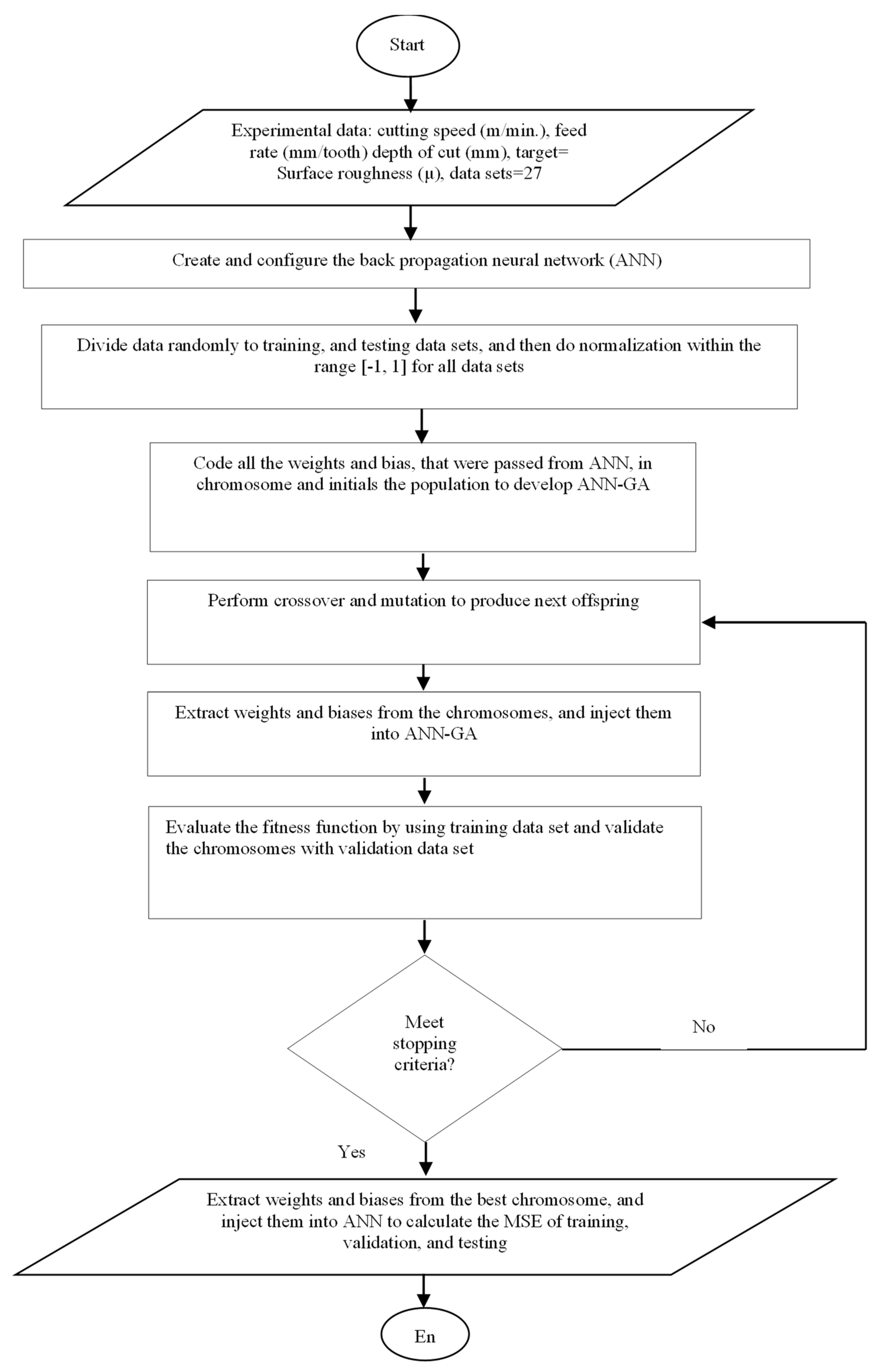
The steps that have been followed to develop the ANN-GA model are summarized as follows:

• Initialize the population of random weights, including biases imported from BPNN. All those weights and biases were coded for the hybrid model. Each chromosome (string) in the population represents the set of weights and biases.
• Later, the crossover and mutation should be carried out for the population to produce the next offspring. The GA performance is determined by adequately selecting its main parameters represented by initial population, crossover, and mutation probability.
• The weights and biases are extracted once the crossover and mutation are finished and injected to the ANN-GA to calculate the MSE for training and validation data.
• If the stopping criterion has been reached, the training should be stopped, and the best chromosome (weights and biases) of GA is extracted and injected again in ANN-GA to calculate the performance (MSE) of the developed model in training, validation, and testing, respectively.

Table 6. GA parameters.

No.	Parameters	Value
1	Population size	20
2	No. of generations	500
3	Crossover probability	0.9
4	Mutation probability	0.01
5	Selection function	Ranking
6	Fitness function	MSE
7	Stopping criterion	Maximum no. of generations exceeded

shows the GA parameters selected based on trial and error to reach the optimum solution. Figure 2 shows the flowchart that illustrates the GA steps that have been followed in this study.

3.2.2. Development of Hybrid ANN-GSA Model

GSA was developed by Rashidi et al. [23] based on the metaphor of gravitational kinematics (Newton’s law), where each particle in the universe attracts each other with force depending on their masses and distance. In this section, GSA has been applied to train BPNN to minimize the mean square error between the targets and desired output. In order to carry out the hybridizing process between GSA and BPNN, some steps should be carried out. Firstly, the weights and biases that were generated from BPNN will be passed to the ANN-GSA hybrid model to initialize the population. Secondly, each agent represents a candidate solution like chromosomes in GA. Thirdly, the fitness function in equation (12) that has been used in the GA hybrid model, is also used here to evaluate the performance in training, validation, and testing phases.

Consider a system with N agents (masses). The position of the ith agent is defined by:

$$Xi=\left(x_i^1,\dots ,x_i^d,\dots ,x_i^n\right) Where i=1,2,3,\dots ,N$$

(13)

where $x_i^d$ presents the position of the ith agent in the dth dimension.

At certain times, ‘t’, the force acting on mass ‘i’ from mass ‘j’, is defined as:

$$F_{ij}^d\left(t\right)=G\left(t\right)\frac{M_{pi}\left(t\right)\times M_{aj}\left(t\right)}{R_{ij}\left(t\right)+\epsilon }\left(x_j^d\left(t\right)-x_i^d\left(t\right)\right)$$

(14)

where M_aj is the active gravitational mass related to agent j, M_pi is the passive gravitational mass related to agent i, G(t) is the gravitational constant at time t, ε is a minor constant, and R_ij(t) is the Euclidian distance between the two agents i and j:

$$R_{ij}\left(t\right)=\Vert X_i\left(t\right),X_j\left(t\right)\Vert 2$$

(15)

It is alleged that the total force that acts on agent i in dimension d is a randomly weighted sum of the dth components of the forces exerted from other agents to provide a stochastic characteristic for the algorithm:

$$F_i^d\left(t\right)={\displaystyle \sum }_{j=1,j\ne i}^{N}ran{d}_j{F}_{ij}^d\left(t\right)$$

(16)

where randj is a random number in the interval [0, 1].

Therefore, by the law of motion, the acceleration of the agent i at time t, and in direction dth, $a_i^d\left(t\right)$ is expressed as in the following:

$$a_i^d\left(t\right)=\frac{F_i^d}{M_{ii}\left(t\right)}$$

(17)

where M_ii is the inertial mass of the ith agent.

Additionally, the next velocity of an agent is thought to be a fraction of its current velocity added to its acceleration. Its position and its velocity, therefore, could be calculated as the following:

$$V_i^d\left(t+1\right)=ran{d}_i\times V_i^d\left(t\right)+a_i^d\left(t\right)$$

(18)

$$X_i^d\left(t+1\right)=X_i^d\left(t\right)+V_i^d\left(t+1\right)$$

(19)

where randi is a standard random variable in the interval [0, 1]. The gravitational constant, G, is initialized at the inception and will decrease with time to control the search accuracy. Simply speaking, G is a function of the initial time (t) and value (G₀):

$$G=G\left(G_0,t\right)$$

(20)

Gravitational and inertia masses are calculated simply by the fitness evaluation. A heavier mass indicates an agent with more efficiency. This means that better agents have heightened attraction and work at a slower pace. By guessing the equality of the gravitational and inertia mass, the values of masses are calculated using the fitness map. Gravitational and inertial masses are updated through the following equations:

$$M_{ai}=M_{pi}=M_{ii}=M_i i=1,2,3,\dots ,N$$

(21)

$$m_i\left(t\right)=\frac{fi{t}_i\left(t\right)-worst\left(t\right)}{best\left(t\right)-worst\left(t\right)}$$

(22)

$$M_i\left(t\right)=\frac{m_i\left(t\right)}{{{\displaystyle \sum }}_{j=1}^N{m}_j\left(t\right)}$$

(23)

where $fi{t}_i\left(t\right)$ represents the fitness values of the agent i at time t, and $worst\left(t\right)$ and $best\left(t\right)$ are defined as follows (for a minimization problem):

$$best\left(t\right)=\mathit{max}fi{t}_j\left(t\right)$$

(24)

$$worst\left(t\right)=\mathit{min}fi{t}_j\left(t\right)$$

(25)

It should be noted that, for a maximization problem, Equations (24) and (25) should be changed to Equations (26) and (27):

$$best\left(t\right)=\mathit{min}fi{t}_j\left(t\right)$$

(26)

$$worst\left(t\right)=\mathit{max}fi{t}_j\left(t\right)$$

(27)

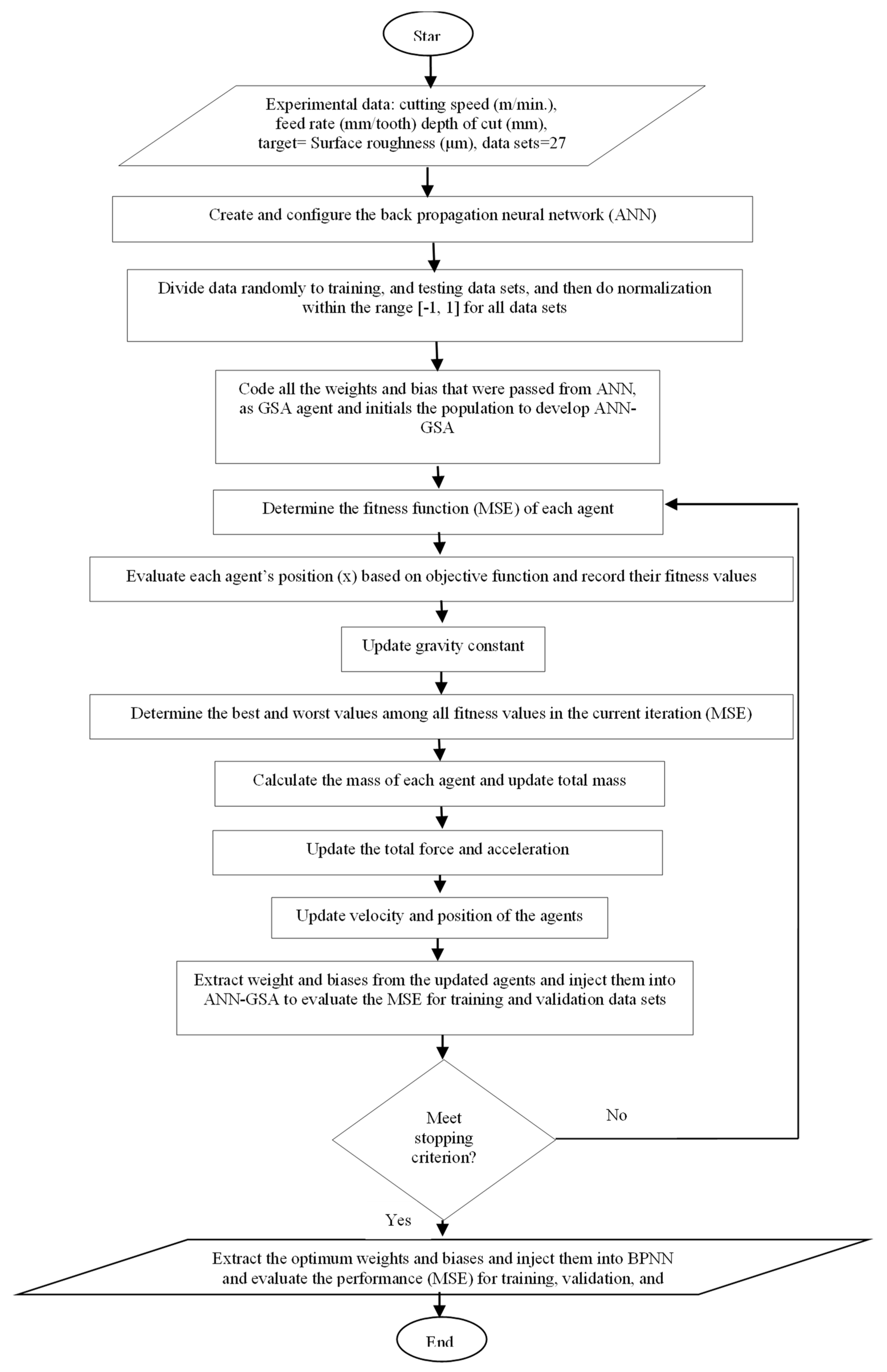
Figure 3 shows the flowchart of how the ANN-GSA hybrid model has been developed, while the steps of ANN-GSA algorithm coding are summarized below:

• Initialize population from sets of weights and biases coming from BPNN.
• Code the weight and bias into agent position vectors.
• Evaluate each agent’s position (x) based on the objective function and record their fitness values.
• Update gravity using the equation.
• Determine the best and worst values among all fitness values in the current iteration based on agent performance (MSE).
• Calculate the mass of each agent and update the total mass value.
• Calculate the total force and then acceleration.
• Update velocity and position of all agents.
• Evaluate the fitness function over the training data set by extracting the weights and biases from updated agents and calculating the mean square error.
• If the stopping criterion has been met, stop and extract the optimum weights and biases and inject them into ANN-GSA and evaluate the performance (MSE) for training, validation, and testing. Otherwise, do steps 3–10.

As in ANN and GA, the control parameters of GSA that judge its performance have been selected based on trial and error.

Table 7. GSA parameters.

No.	Parameters	Value
1	Population size	30
3	Gravity constant	100
4	Fitness	MSE
5	Maximum no. of iterations	500
6	Stopping criterion	Maximum iterations reached

shows the GSA control parameters. It can be seen from Figure 3 that the information is sent out and sent back between GSA and ANN to reach the optimum solution. The same thing happened in ANN-GA in the training phase.

4. Results and Discussion

This section consists of two parts. The first one is the analysis of experimental results by using ANOVA analysis with design expert software. Also, the same software was used to find the optimum cutting conditions that achieve minimum surface roughness. The second part is the development of hybrid intelligent models of ANN-GA and ANN-GSA based on experimental data to predict the surface roughness of the Ti6Al4V machined surface.

4.1. Surface Roughness Analysis for PVD Coated Tools

The surface roughness was evaluated to investigate the significant factors that affect the surface roughness when end milling titanium Ti-6Al-4V with PVD insert under dry cutting conditions. The surface finish gradually deteriorated as the wear at the cutting edges increased. Taguchi method was applied in this study to investigate the most significant factors and their contributions by using design expert software. The same software was used to determine the optimum cutting conditions that achieve minimum surface roughness. The experiment results are shown in

Table 8. Experimental data for surface roughness of PVD cutting tool.

No.	Cutting Speed (m/min.)	Feed Rate (mm/Tooth)	Depth of Cut (mm)	Surface Roughness (μ)
1	50	0.1	1	0.352
2	50	0.15	1.5	0.793
3	50	0.2	2	1.556
4	77.5	0.1	1	0.512
5	77.5	0.15	1.5	0.799
6	77.5	0.2	2	1.495
7	105	0.1	1	0.305
8	105	0.15	1.5	0.579
9	105	0.2	2	1.194
10	50	0.1	1.5	0.578
11	50	0.15	2	0.676
12	50	0.2	1	0.871
13	77.5	0.1	1.5	0.360
14	77.5	0.15	2	0.760
15	77.5	0.2	1	1.037
16	105	0.1	1.5	0.452
17	105	0.15	2	0.872
18	105	0.2	1	0.875
19	50	0.1	2	0.370
20	50	0.15	1	0.593
21	50	0.2	1.5	0.812
22	77.5	0.1	2	0.509
23	77.5	0.15	1	0.638
24	77.5	0.2	1.5	0.832
25	105	0.1	2	0.474
26	105	0.15	1	0.495
27	105	0.2	1.5	0.945
Maximum value				1.556
Minimum value				0.305
Average value				0.744609

.

Analysis of variance (ANOVA) clarifies which factor has many effects on response and also reveals the significance of the model that has been built. Furthermore, the contributions of each factor and their interaction are also shown in

Table 9. Analysis of variance (ANOVA) for surface roughness using PVD cutting tools.

Source	Sum of Squares	Degree of Freedom	Mean Square	F Value	Prob > F	Contribution %
Model	2.51757	18	0.139865	7.233067	0.0038	-
A	0.031363	2	0.015681	0.81096	0.4779	1.173645
B	1.831244	2	0.915622	47.35106	<0.0001	68.52779
C	0.3065	2	0.15325	7.92527	0.0127	11.46967
AB	0.003866	4	0.000967	0.049983	0.9943	0.144673
AC	0.032945	4	0.008236	0.425933	0.7864	1.232844
BC	0.311652	4	0.077913	4.02924	0.0445	11.66246

. The model adequacy should be checked because an inadequate model will result in misleading conclusions.

By investigating Table 9, the Model F-value of 7.233067 implies the model is significant. There is only a 0.38% chance that a “Model F-value” this large could occur due to noise. Values of “Prob > F” less than 0.05 indicate model factors are significant. Since the “Prob > F” value of feed rate (B) is less than 0.0001, that means this factor is significant. Similarly, the 0.0127 value of depth of cut (C) is less than 0.05, and it reveals its significance. Further, the feed rate and cut depth (BC) interaction are also significant. Values greater than 0.1 indicate the model factors are not significant. Therefore, in this case, the cutting speed (A), the interactions (cutting speed and feed rate (AB), cutting speed, and depth of cut (AC)) are insignificant due to their large “Prob > F” values, which are greater than 0.1. The R2 of this model is 0.9421, and it is considered a good value. The mean square error value is 0.015359226. Adeq Precision measures the signal-to-noise ratio. A ratio greater than 4 is desirable. In this case, the ratio of 9.724 indicates an adequate signal. Hence, this model can be used to navigate the design space. 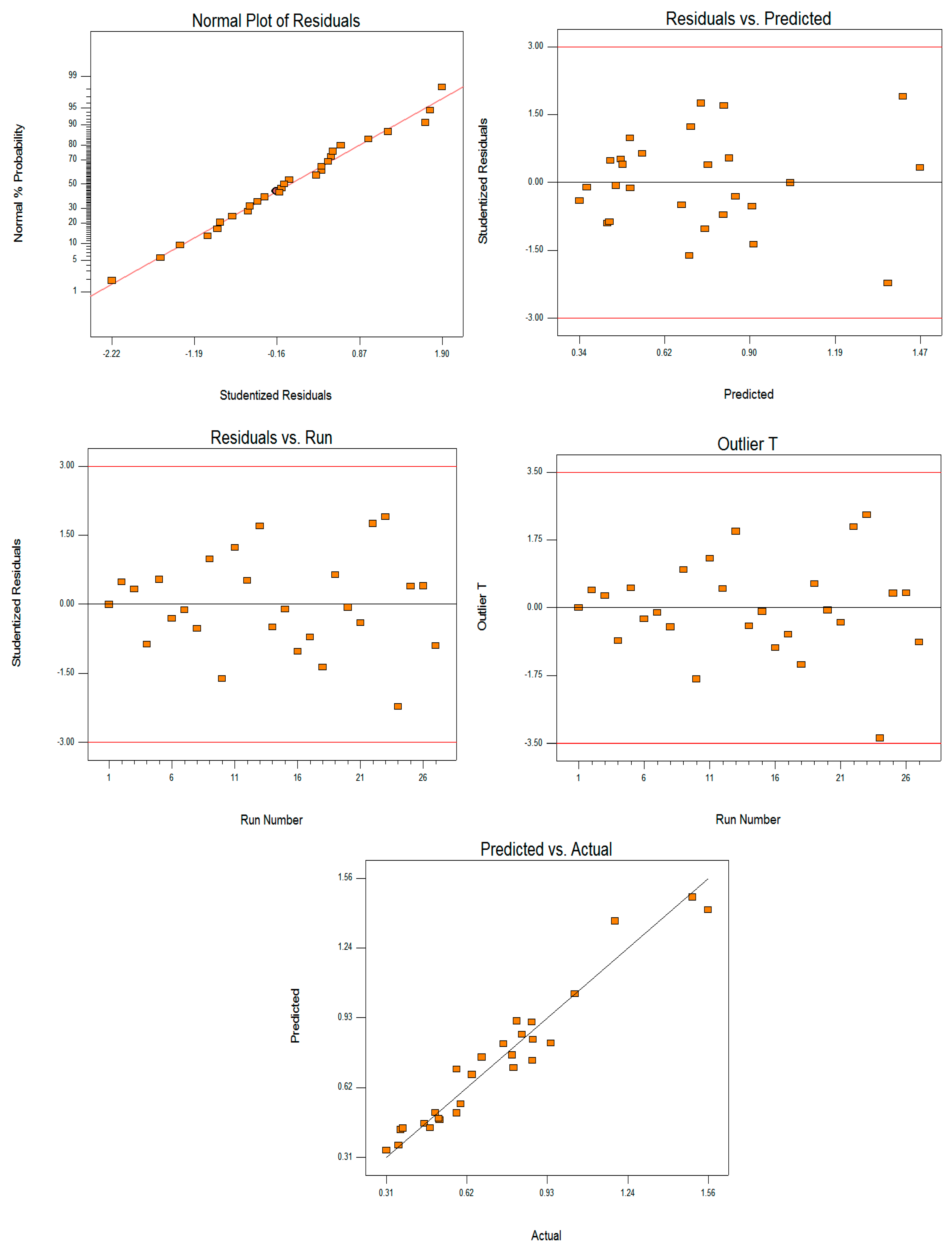By looking at the same table (Table 9), the feed rate’s high contribution (68.52779) compared with depth of cut and cutting speed is clear. This explains why feed rate is the most significant factor, followed by the depth of cut. Moreover, design expert software provides residual graphs as part of the model statistical report. The five graphs in Figure 4 of normal %probability, residuals versus predicted, residual versus run, outlier, and predicted versus actual plots, gave an indication of normal distribution for the data and verified that this model satisfied goodness of fit.

4.1.1. Effects of Cutting Process Parameters on Surface Roughness

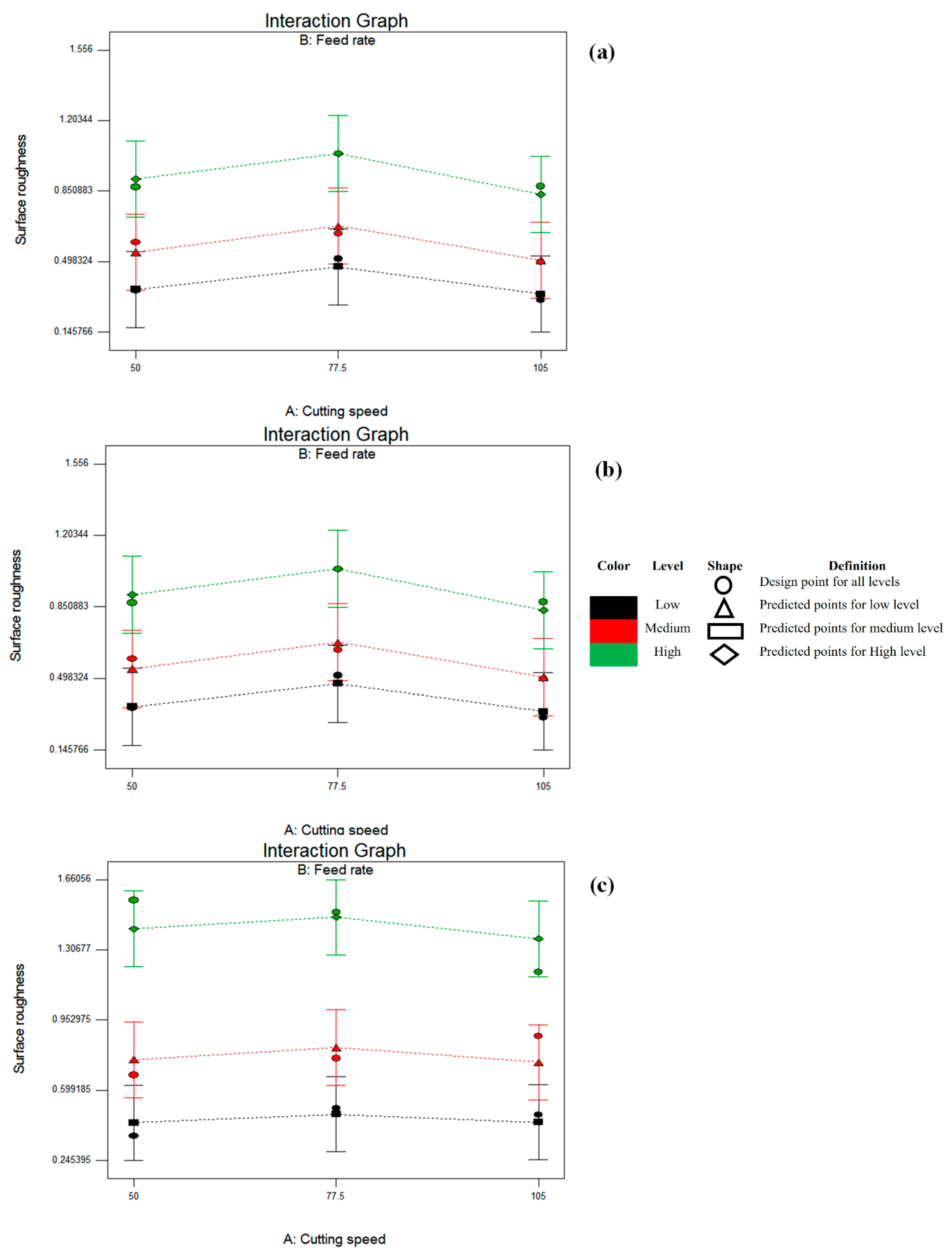
One of this study’s objectives is to investigate the effect of cutting parameters on output response represented by surface roughness. Interaction graphs are generated using design expert software to do this task. Figure 5, Figure 6 and Figure 7 represent the interaction graphs of cutting speed-feed rate, cutting speed-depth of cut, and feed rate-depth of cut, respectively. Each graph consists of three plots to clarify the effect of two factors while keeping the third constant. Circular points represent the design points, while the square, triangle, and rhomboid refer to the predicted points of the model. For both design and predicted points, the cutting conditions’ low, medium, and high levels are drawn by black, red, and green colors, respectively. The dotted lines connect the predicted points. Figure 5 revealed that the cutting speed effect is less dominant than the feed rate. For the depth of cut = 1 mm, the low value of Ra was achieved at low feed rate with high cutting speed (design point 7 with 0.305333 μ). Moving to the second plot of Figure 5, the depth of cut was held at 1.5 mm, and the minimum roughness value was obtained with a medium cutting speed (77.5 m/min.) with low feed rate (design point 13 with 0.36 μ). The third plot of the same figure revealed the high impact of feed rate when a high depth of cut accompanies it. Obtaining low surface roughness for this plot is located at the left bottom corner (design point 19 with 0.369667 μ). This result is statistically logical by considering the high contribution percentage of feed rate (68.53) while cutting speed contributed only 1.17.

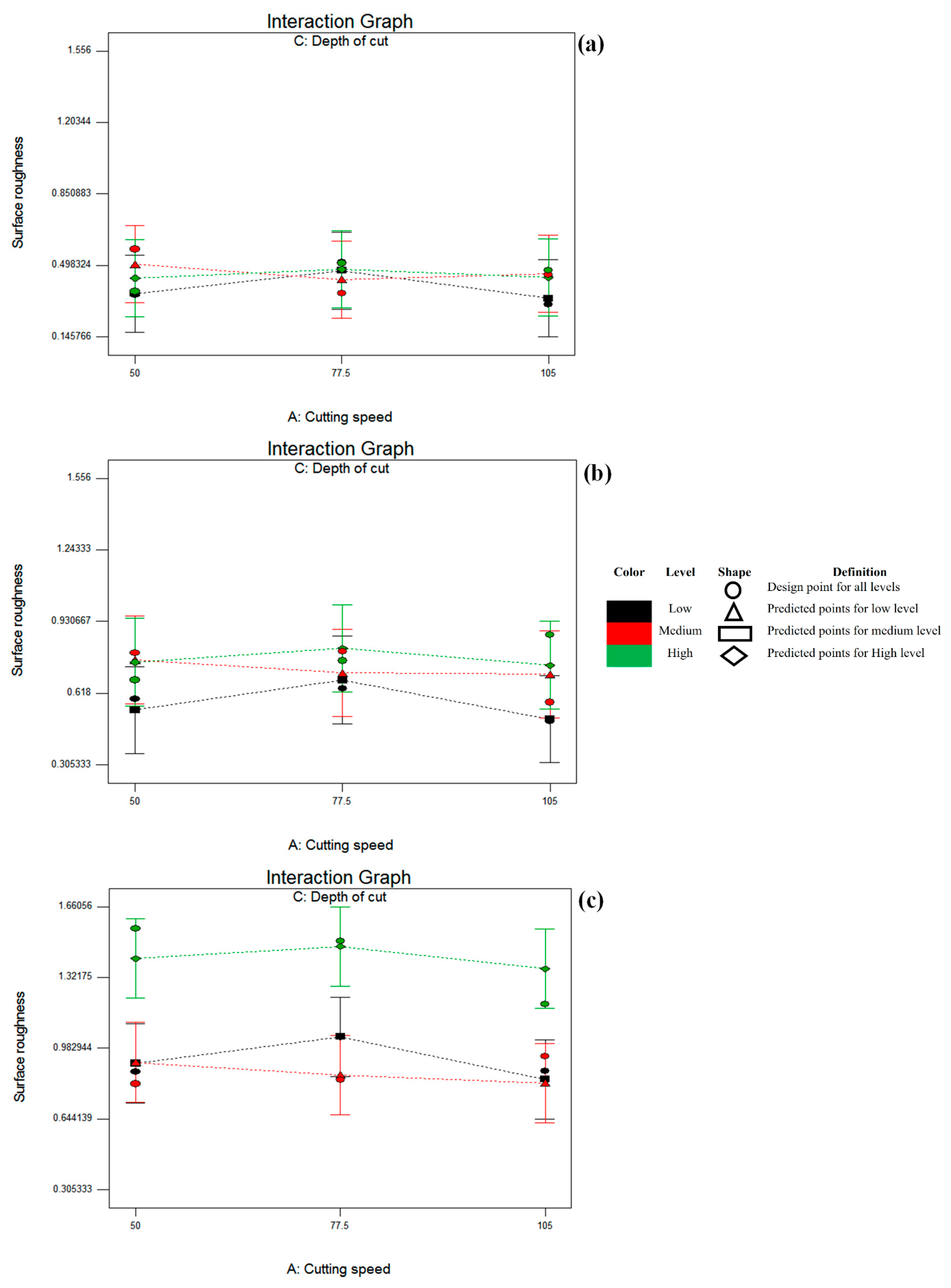
Figure 6 shows the effect of cutting speed and depth of cut with feed rate holding values of 0.1, 0.15, and 0.2, respectively. For low feed rate, the Ra value ranged from 0.30533 to 0.577 μ (design points 7 and 10) for all cutting ranges of cutting speed and depth of cut. For depth of cut 1 and 2 mm with low feed rate, the surface roughness value increases over low to medium cutting speeds and decreases towards high cutting speed. However, the reverse is found for 1.5 mm depth of cut with low feed rate. Hence, a low surface roughness value for medium cutting speed is achieved at a low feed rate accompanied with a medium depth of cut. At a high depth of cut with a medium feed rate, the Ra value increases with the cutting speed from 50 to 105 m/min. 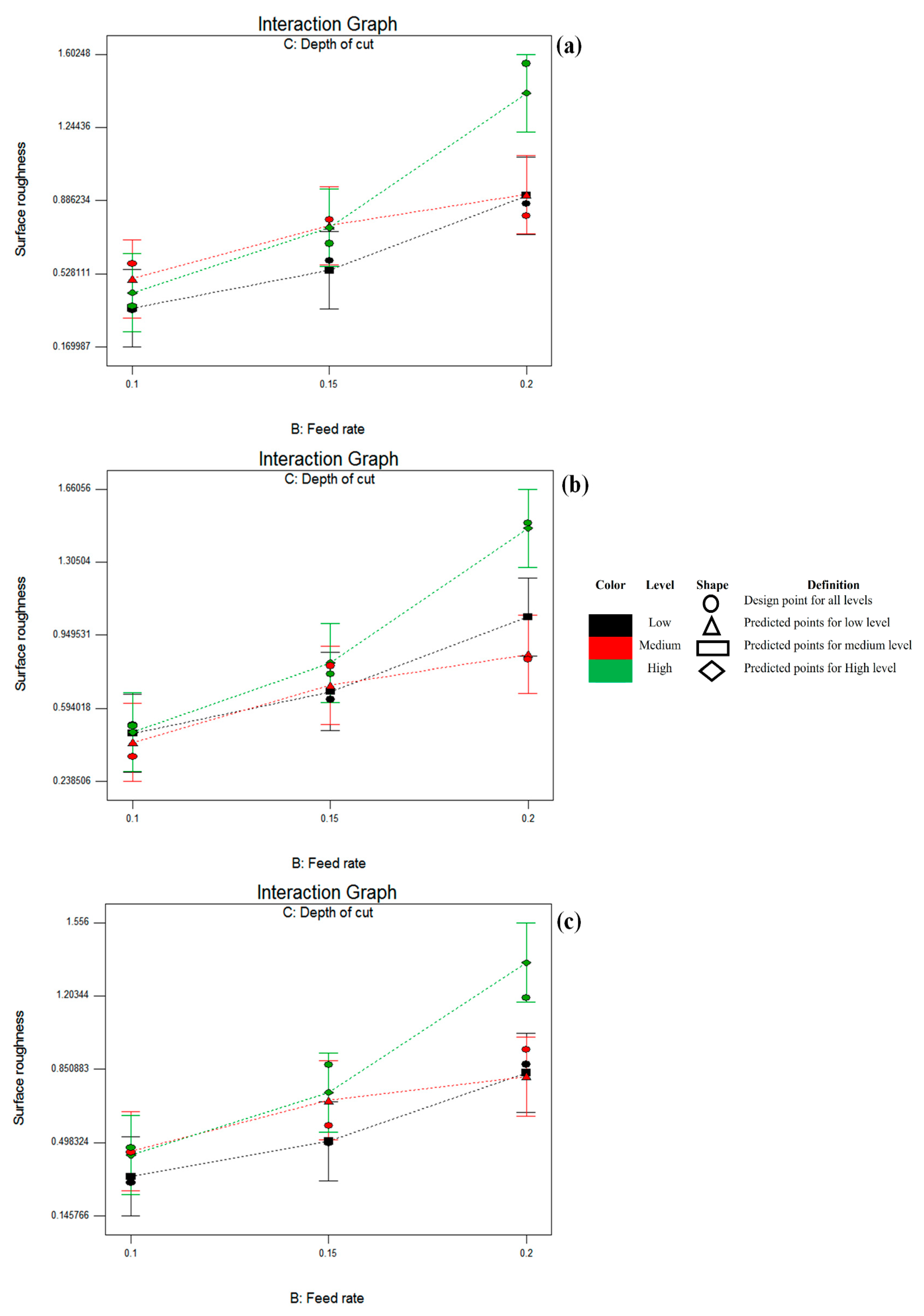The lowest roughness value for this range is obtained at low depth of cut and high cutting speed (design point 26 with 0.495 μ). The maximum surface roughness value is 1.506 μ and is obtained at a high feed rate and depth of cut with low cutting speed (design point 3). It is evident from Figure 7 that the combined effect of feed rate and depth of cut is diverse at different cutting speeds. The roughness values are increasing with the increase of feed rate and depth of cut.

To sum up, the results and analysis revealed that the most significant factor affecting the surface is feed rate, followed by the depth of cut. Better surface roughness could be achieved at both low and high cutting speed and low feed rate and depth of cut. Also, if the cutting speed, feed rate, and depth of cut are set on medium, low, and medium levels, respectively, this could achieve a low surface roughness value. In the next section, the optimum value of surface roughness and cutting conditions can also be found using design expert software.

The surface roughness was improved with a low feed rate (0.1 mm/tooth), particularly when it is accompanied by a high cutting speed. However, worse surface roughness was obtained with a high feed rate and depth of cut (design point 3), especially when accompanied by low cutting speed.

The influence of cutting speed on machined surface roughness is quite complex and dependent on the material type of the cutting tools. For example, for relatively low hardness and fracture toughness cutting tools, the roughness value increases as the cutting speed increases. On the other hand, the behavior is different for the carbide tool, either coated or uncoated. The surface roughness decreases as cutting speed increases. During machining, the temperature in the cutting zone is high due to friction between cutting tool and the workpiece, which generates considerable heat. This makes the machined surface softened, resulting in a fine surface. The worst value of surface roughness for PVD cutting tools is 1.556 µm. High feed rate produces marks on the surface being machined, thus producing a coarser surface with a higher roughness value. Moreover, a high feed rate may cause fracture of the cutting edge and create a rough surface.

The temperature rises in metal cutting result from two heat sources. The first is the frictional heat source due to friction at the tool-chip interface. The second one is the shear zone heat source which results from the development of plastic deformation at the shear plane. Therefore, the machining of titanium alloy requires a cutting tool with high thermal conductivity and low reactivity to increase the surface contact area at the tool-chip interface, which results in the enlargement of the heat affected zone, which accelerates the heat dissipation away from the cutting zone. In other words, as chip/tool contact length increases, the heat-affected area increases also. Further, it needs tougher and harder tool grades to withstand the dynamic load [39].

Though straight tungsten carbide tools have revealed good performance in titanium machining, they suffer from rapid crater wear and plastic deformation of the cutting edges at higher cutting speed. This resulted in heat generation close to the cutting insert nose. As a result, the heat-affected zone will be minimal due to the concentration of heat in a small area. In other words, it accelerates the plastic deformation when it is accompanied with a high dynamic load due to high cutting speed, feed rate, and depth of cut. Consequently, it causes chipping at the cutting edge and rapid tool failure, producing a poor surface finish. Furthermore, metallurgical changes due to diffusion between the cutting tool and Ti6Al4V work part result in increasing micro-hardness and microstructure alteration. This explains why this study utilized the PVD coated tool instead of the uncoated cutting tool [40].

On the other hand, the PVD coated tool performs differently by producing a good surface finish compared with an uncoated tool. Metallurgists play a significant role in serving engineering and science disciplines by innovating new materials that could meet the demand. Here, the PVD coated tool is characterized by aspects that make it achieve good machining performance compared with an uncoated tool. The coatings were developed for cutting tools to provide significant properties and aspects that allow cutting tools to cover a wide range of machining different materials. For example, coatings have good wear resistance and less affinity towards the material being machined.

Meanwhile, they keep their hot hardness at a high temperature. Furthermore, the coating layer minimizes material hardness change. Meanwhile, it has low thermal conductivity, meaning it dissipates less heat for the substrate and acts as a thermal barrier. Also, it has a low coefficient of friction which in turn reduces frictional heat. Because of the wearing out of the cutting tools due to the chemical reactivity of titanium alloy during the machining process, the coating layer provides excellent chemical stability and wear resistance. TiAlN that exists in the PVD tool has the above properties and acts as a dry lubricant, chemical, and thermal barrier for the substrate. Therefore, the findings of the PVD coated tool provided better results and improved the machining performance of carbide tools, especially with high-speed machining [41].

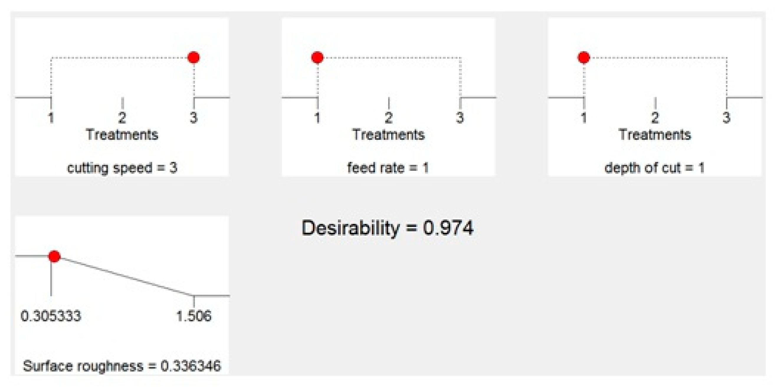
4.1.2. Optimization of End Milling Parameters

The previous subsection investigated the effect of milling parameters on machinability index (surface roughness) when end milling Ti6Al4V alloy with PVD coated cutting tool under dry cutting conditions. The interaction graphs could indicate optimum cutting conditions that achieve minimum surface roughness, but this could not be defined and specified well from those graphs. Therefore, the optimum settings with minimum surface roughness can be determined by using the optimization solution provided by the design expert software. The criterion that has been followed is holding all the cutting conditions within the range while maintaining the surface roughness at a minimum. Following this criterion achieved minimum surface roughness with 0.336346 μ. The optimum settings that led to this lowest value are high cutting speed (105 m/min), low feed rate (0.1 mm/tooth), and low depth of cut (1 mm), respectively. Confirm test using these optimum settings obtained minimum surface roughness with 0.25 µm. The ramp plot of optimum conditions is shown in Figure 8, with a desirability of 0.974.

Table 10. Optimum settings of cutting conditions.

Parameters and Reponses	Objective	Lower Limit	Upper Limit	Optimum Settings for Cutting Parameters with 0.974 Desirability
Cutting speed	is in range	50	105	105
Feed rate	is in range	0.1	0.2	0.1
Depth of cut	is in range	1	2	1
Surface roughness	minimize	0.305333	1.506	0.335976

shows the optimum setting and followed criterion.

4.2. Prediction of Surface Roughness by Using Back Propagation Neural Network Algorithm (BPNN)

Modeling the machining process is an important issue that has attracted researchers in the last few decades. Due to its complexity and nonlinearity, statistical techniques could not handle this relationship. Artificial neural network (ANN) exists to solve this kind of problem. However, ANN has some parameters that need adjusting. The central idea of the artificial neural network is that such parameters can be tuned so that ANN achieves interesting behavior and exhibits good output close to actual targets.

The experimental data sets in Table 8 have been used in training, validating, and testing of the BPNN model. It has three inputs and one output representing the three cutting parameters and surface roughness, respectively.

These data sets are divided to the following subsets:

• 70% for training (19 patterns).
• 15% for validating (4 patterns).
• 15% for testing (4 patterns).

Feed forward back propagation neural network is commonly used by researchers due to its accuracy compared with other networks [38]. It can be used for solving prediction and pattern recognition problems. Therefore, it is like a backbone for neural networks. The data sets have been divided randomly into three subsets: training, validation, and testing set, with division percentages of 70%, 30%, and 30%, respectively. Based on this division, 19, 4, and 4 samples will be used in the training, validation, and testing phases, respectively. These data sets with input-target pairs should be normalized before training to avoid computation problems. The normalization range for the input/target pair is -1 to 1, and the Levenberg–Marquardt is selected as the training function because it is characterized by fast convergence. The most commonly used transfer functions are logsig, tan sig, and purelin functions. The tan sig is differentiable and constantly used in hidden layer and squashes the net value between −1 and 1. For pattern recognition and classification, it is also used in the output layer. However, in this case study, purelin function has been used because the problem is function approximation and fitting. The learngdm is the gradient descent with momentum, weight, and bias learning function with learning rate and momentum 0.01 and 0.9, respectively. The performance function is mean square error (MSE), which can be calculated by taking the average of square error for the targets-desired outputs pairs. Single hidden layer was used and neurons number was changed from 1 to 20.

Full analysis of developed BPNN models should be done after the training, validation, and testing phases to assess and evaluate the performance and accuracy of each model. This critical step aims to select the best model for predicting surface roughness of end milled Ti6Al4V alloy with PVD-coated cutting tools under dry cutting conditions.

After finishing the training, validation, and testing phases, their results are tabulated and plotted to do the analysis. The accomplished results are shown in

Table 11. Statistical measures of mean square error of ANN models.

No. of Neurons	MEAN			MEDIAN			STDV			BEST
	Training	Validation	Testing	Training	Validation	Testing	Training	Validation	Testing	Training	Validation	Testing
1	0.040206	0.042626	0.051391	0.023684	0.027	0.036452	0.039337	0.060298	0.043889	0.007096	0.004081	0.009791
2	0.031045	0.033027	0.051078	0.015201	0.028109	0.029039	0.036435	0.022642	0.056132	0.002297	0.005117	0.002219
3	0.028323	0.026508	0.060675	0.024069	0.01347	0.039685	0.016904	0.027694	0.051952	8.21 × 10−3	3.57 × 10−3	8.17 × 10−3
4	0.026437	0.033058	0.047803	2.31 × 10−2	0.016225	0.023347	2.08 × 10−2	3.96 × 10−2	4.41 × 10−2	2.02 × 10−3	3.74 × 10−3	3.92 × 10−3
5	3.58 × 10−2	0.03247	0.089984	1.07 × 10−2	2.41 × 10−2	3.65 × 10−2	7.98 × 10−2	0.03693	0.131291	1.27 × 10−3	5.20 × 10−3	6.64 × 10−3
6	3.58 × 10−2	0.03247	0.089984	1.07 × 10−2	2.41 × 10−2	3.65 × 10−2	0.079828	0.03693	1.31 × 10−1	1.27 × 10−3	5.20 × 10−3	6.64 × 10−3
7	0.023978	0.037127	0.065278	1.51 × 10−2	3.17 × 10−2	3.54 × 10−2	0.037428	0.028924	0.055127	6.75 × 10−5	5.78 × 10−3	1.21 × 10−2
8	2.53 × 10−2	6.97 × 10−2	0.110559	2.40 × 10−2	5.12 × 10−2	1.15 × 10−1	2.08 × 10−2	0.059071	0.068551	8.13 × 10−6	1.74 × 10−3	5.76 × 10−3
9	2.89 × 10−2	0.063191	0.091423	1.74 × 10−2	3.81 × 10−2	8.65 × 10−2	3.06 × 10−2	5.47 × 10−2	7.25 × 10−2	4.85 × 10−13	3.24 × 10−3	4.47 × 10−3
10	1.65 × 10−2	0.06648	0.092383	1.25 × 10−2	4.61 × 10−2	6.54 × 10−2	1.61 × 10−2	0.063356	0.085663	2.07 × 10−14	2.08 × 10−3	1.14 × 10−2
11	2.62 × 10−2	0.091054	0.150916	2.28 × 10−2	4.41 × 10−2	8.08 × 10−2	0.024622	0.103321	0.172433	3.23 × 10−14	1.68 × 10−3	1.37 × 10−2
12	6.71 × 10−2	1.01 × 10−2	9.97 × 10−1	6.73 × 10−3	8.97 × 10−2	1.00 × 10−1	3.30 × 10−1	0.07527	0.149881	1.11 × 10−5	1.66 × 10−2	2.26 × 10−2
13	2.10 × 10−2	0.071451	0.123736	1.35 × 10−2	5.64 × 10−2	8.67 × 10−2	2.27 × 10−2	4.57 × 10−2	1.30 × 10−1	5.66 × 10−13	4.54 × 10−3	5.63 × 10−3
14	4.56 × 10−2	0.09757	0.15118	6.85 × 10−3	8.10 × 10−2	1.33 × 10−1	1.51 × 10−1	7.92 × 10−2	1.55 × 10−1	4.77 × 10−21	1.61 × 10−2	9.47 × 10−3
15	1.89 × 10−2	0.137334	0.137201	1.02 × 10−2	9.23 × 10−2	1.21 × 10−1	2.63 × 10−2	0.148896	0.110262	4.24 × 10−6	8.90 × 10−3	4.90 × 10−3
16	1.38 × 10−2	0.119961	0.191153	1.07 × 10−2	1.01 × 10−1	1.60 × 10−1	1.55 × 10−2	7.77 × 10−2	1.48 × 10−1	2.78 × 10−19	3.13 × 10−2	3.21 × 10−2
17	7.09 × 10−3	0.116351	0.155743	1.12 × 10−5	1.19 × 10−1	1.34 × 10−1	1.13 × 10−2	0.079677	0.099157	3.53 × 10−21	8.31 × 10−3	1.79 × 10−2
18	9.82 × 10−3	0.120316	0.179504	5.88 × 10−3	1.02 × 10−1	1.24 × 10−1	1.18 × 10−2	0.083271	0.203434	1.45 × 10−20	2.37 × 10−2	8.86 × 10−3
19	1.70 × 10−1	0.139485	0.160501	8.14 × 10−3	1.07 × 10−1	1.28 × 10−1	6.90 × 10−1	0.1102	0.110138	2.89 × 10−19	1.02 × 10−2	5.50 × 10−3
20	6.93 × 10−3	0.161342	0.219837	2.49 × 10−3	1.41 × 10−1	1.83 × 10−1	0.011261	0.128847	0.149723	3.73 × 10−18	2.95 × 10−3	2.01 × 10−2
minimum	0.006931	0.010072	0.047803	1.12 × 10−5	0.01347	0.023347	0.011261	0.022642	0.043889	3.53 × 10−21	0.001676	0.002219

, where twenty neural network structures have been developed with single hidden layers and variable neurons ranging from 1–20. In general, a single hidden layer is enough if it achieves an accurate result. Otherwise, it is better to try two or more hidden layers. According to the literature related to machining processes, no authors used more than three layers. The number of layers and their neurons is proportional to the degree of complexity and nonlinearity of the problem under investigation. Hence, the performance of a single hidden layer is satisfactory; there is no need to try more hidden layers because it could potentially do input-output mapping in this case study. The number of hidden layers and neurons is case sensitive because their improper selection may lead to either under-fitting or over-fitting. The main objective is to achieve good fitting between the targets and the desired output. This good fitting oscillates between under and over-fitting points. Therefore, taking care is required for this critical issue.

Before starting the analysis, it is necessary to specify the criterion that should be followed to select the best models. In this study, the performance of each network structure has been assessed based on the criterion that picks up the minimum MSE value in testing. The testing phase checks the neural network’s generalization by detecting the output of unseen input data not included in the training phase. However much the neural network outputs are close or near to the testing targets is how much the MSE is minimized.

It is known that the generated weight matrix and biases values are not the same for each run. In other words, each run will give different results. To overcome this issue, it is better to make multiple runs for each network structure and evaluate all the runs by using common statistical measures like mean, median, standard deviation, and the best.

The best model selection is based on minimum MSE among all best testing values to get maximum prediction accuracy. By checking the statistical measures of MSE values in Table 11 for all twenty neural networks and applying the above criterion, it can be concluded that the best model for the PVD tool is 3-2-1 because it accomplished minimum MSE (0.002219) in testing. This best model consists of a single hidden layer with two neurons. The three and one stand for cutting parameters and surface roughness, respectively. More investigation for these tables reveals that the mean and best MSE in testing were no less than 0.05 and 0.002, respectively. This means that the best MSE is less than the mean by more than ten times.

Regarding the median, it picks up the mid value from all twenty values of each network structure. The twenty values refer to the twenty runs of each network structure. In general, its values are no less than 0.02 and 0.04. This implies that the lower half of twenty runs has achieved relatively high MSE. The dispersion of observations (MSE of each run for each network structure) around the mean represents the standard deviation. In general, the trend of mean, median, standard deviation, and best MSE was good.

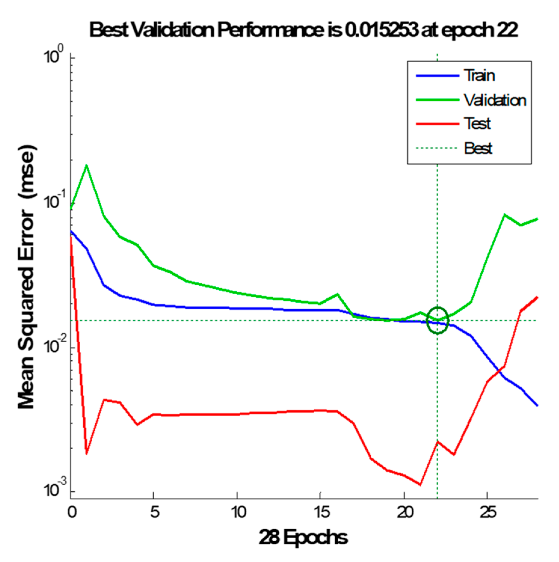
The performances of the best models are shown in Figure 9. The best validation mean square error is accomplished at epoch 22 with 0.015253, which is indicated with a green circle and dotted line. This figure shows the training, validation, and testing performance curves. However, Figure 9 shows no significant problems with the training curves. The trend of validation and testing curves seems similar from the viewpoint of decreasing and increasing their errors. If the testing curve had increased and jumped significantly before the validation curve increased, it would have implied some overfitting might have occurred. It can be seen from this figure that the trend of the testing curve is located under the training and validation curves. This explains why a model 3-2-1 has achieved R testing values of 0.9951 (Figure 10). In other words, the mean square error of testing is less than the training and validation ones and this confirms the generalization of the developed models through recognizing the output of unseen input data that were not involved in training and validation.

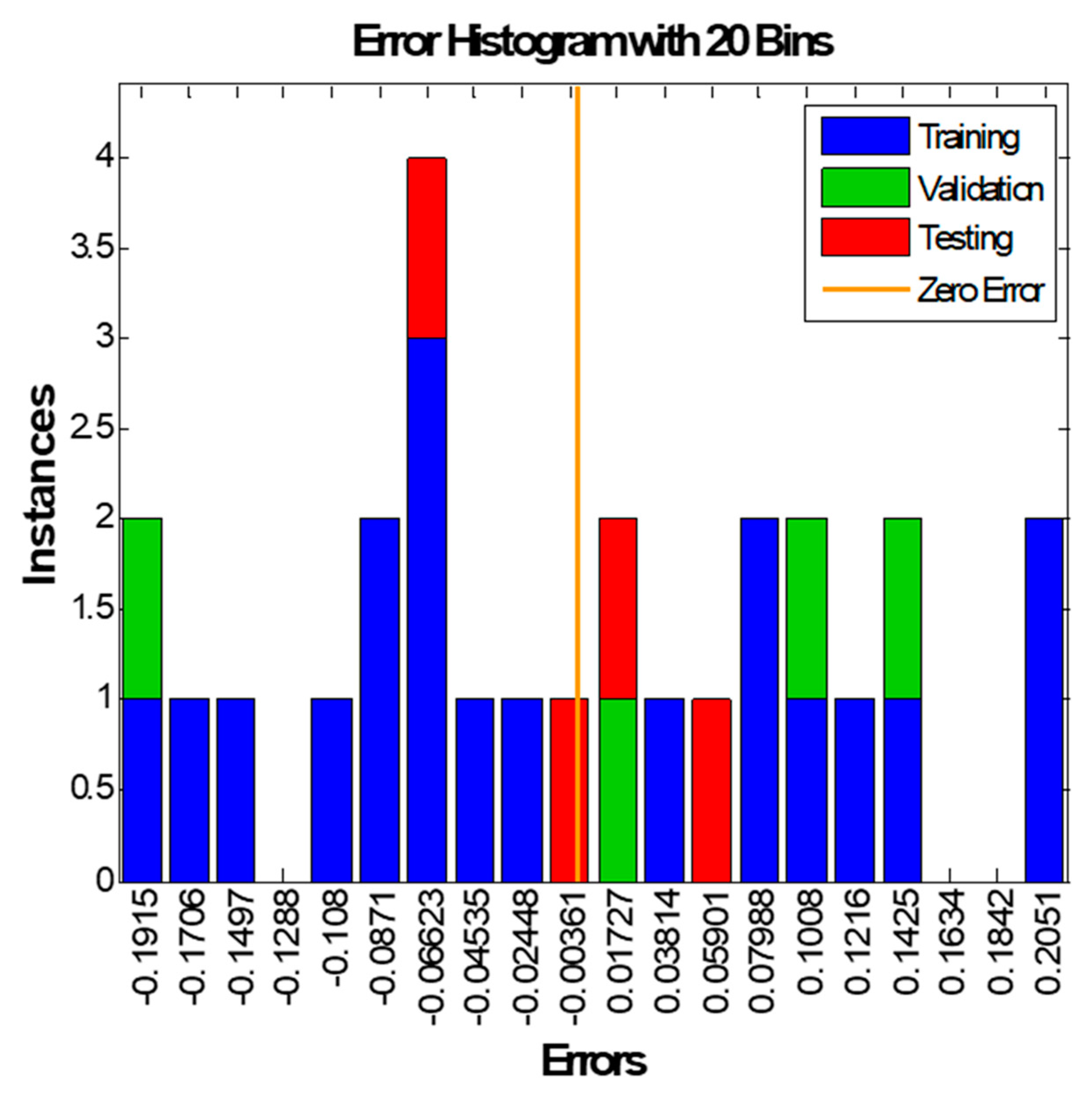
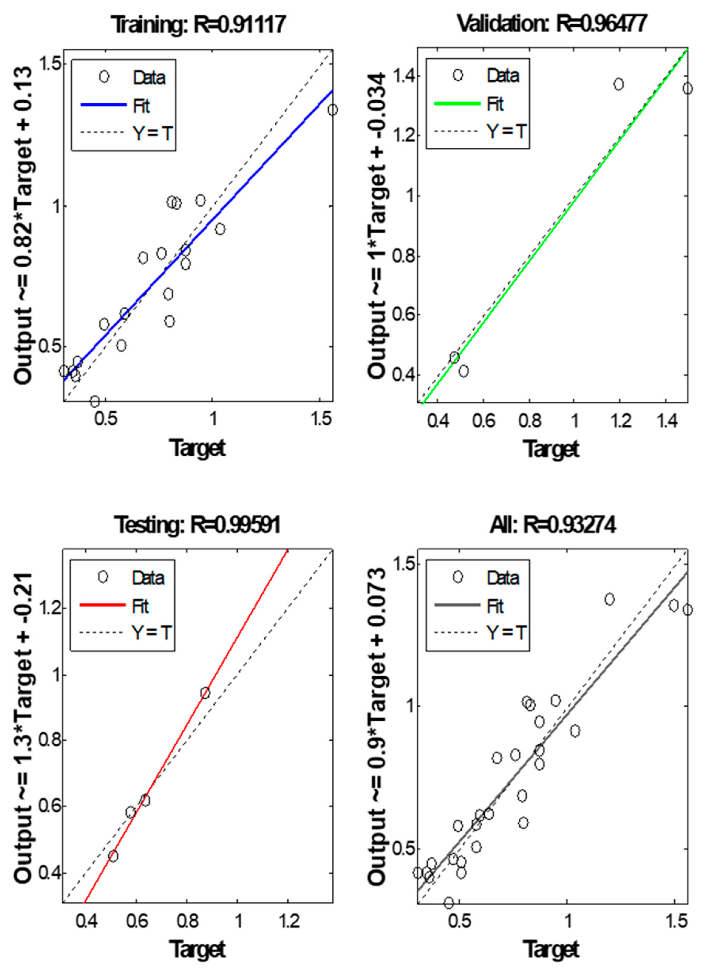
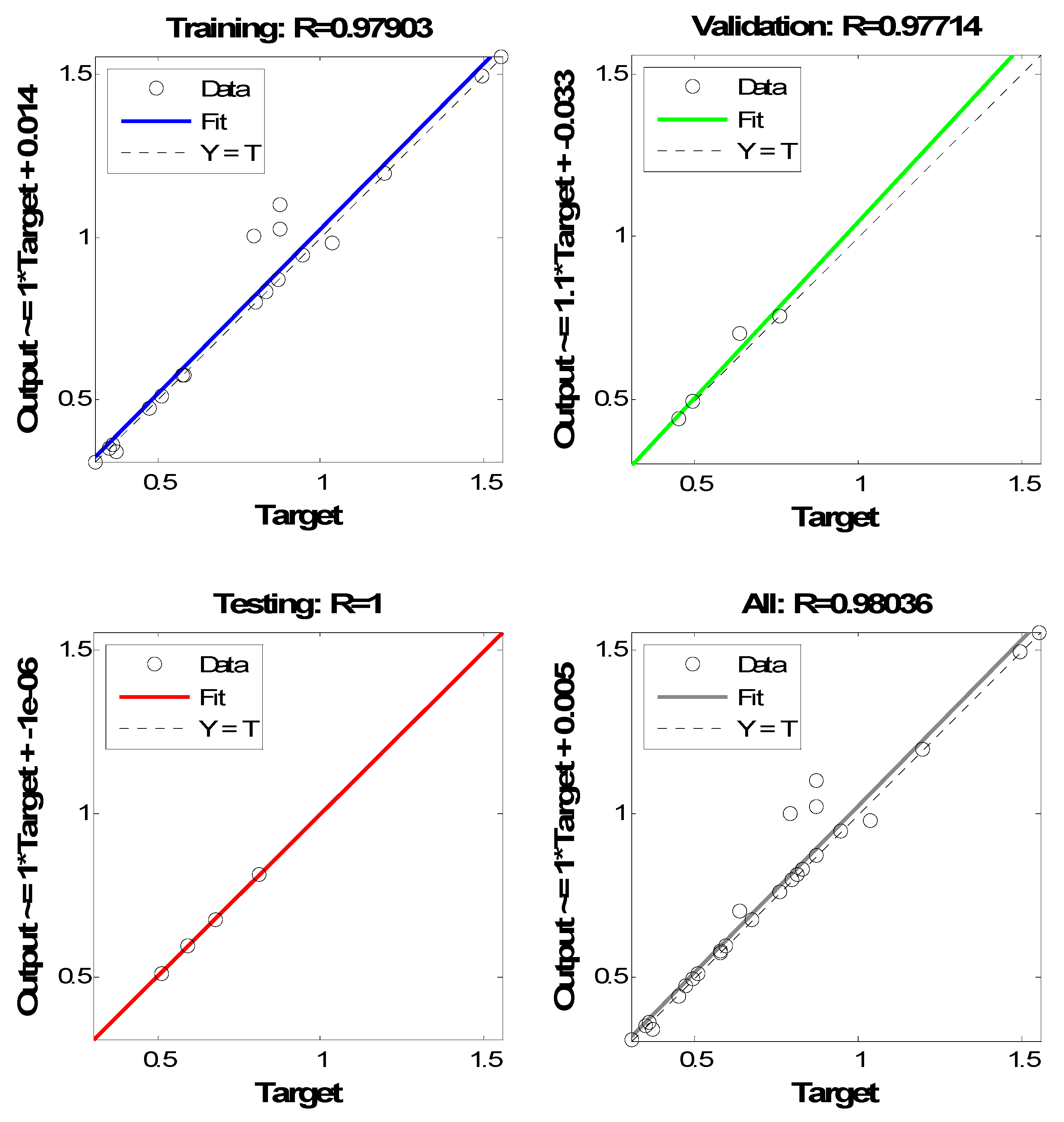
Figure 11 shows the histogram plots of the 3-2-1 model. It consists of twenty bins or intervals. The training, validation, and testing errors are assigned blue, green, and red bars. These figures clarify that the PVD tool’s testing error ranges from −0.06623–0.5901. Figure 10 shows the regression plots for training, validation, testing, and all with their respective values. The R values in testing are greater than 0.9, which refers to the good fit between the targets and the output in testing. Most of the desired outputs with open circles are located around the best fit line; hence, there is no big scattering in testing concerning the targets.

4.3. Prediction of Surface Roughness by Hybrid Neural-Genetic Algorithm Model

Fitness function evaluated all the chromosomes that stood for weights and biases. Probability-based is the criterion applied for chromosome selection for breeding (crossover) and mutation operation. After each generation, the poor solutions should be eliminated to keep the population size fixed. This genetic operation was performed until it reached the maximum generation value. The stopping criterion is reaching maximum generation. At this point, the final solution has been achieved, and the best chromosome (weights and biases) will be extracted and injected into ANN-GA again to evaluate the performance measure (MSE) in training, validation, and testing.

The main aim of this model is to minimize the fitness function as much as possible to improve the BPNN performance. The optimum weight and bias values represent the optimum mean square error.

Table 12. Statistical measures of mean square error of ANN-GA models.

No. of Neurons	MEAN			MEDIAN			STDV			BEST
	Training	Validation	Testing	Training	Validation	Testing	Training	Validation	Testing	Training	Validation	Testing
1	0.020043	0.007849	0.029546	0.019466	0.004424	0.026594	0.00318	0.00864	0.021852	0.014345	0.001115	0.006307
2	0.012002	0.003439	0.030103	0.010262	0.003362	0.025057	0.005703	0.002056	0.022737	0.005005	5.23 × 10−4	0.006279
3	0.008663	0.001341	0.046969	0.006618	8.24 × 10−4	0.038099	0.004042	0.001297	0.041109	0.00453	1.78 × 10−4	0.006969
4	0.006721	0.001131	0.033635	0.006342	7.17 × 10−4	0.02975	0.002543	9.43 × 10−4	0.02044	0.003783	2.04 × 10−4	0.007055
5	0.006932	0.001128	0.045651	0.006282	7.44 × 10−4	0.036915	0.003187	0.001398	0.035331	0.003433	7.43 × 10−5	0.006348
6	0.006272	4.65 × 10−4	0.071438	0.004961	3.58 × 10−4	0.051409	0.004003	3.27 × 10−4	0.050351	0.002535	1.14 × 10−4	0.01378
7	0.00604	4.86 × 10−4	0.066006	0.005912	4.24 × 10−4	0.047141	0.00239	2.97 × 10−4	0.052029	0.001125	2.16 × 10−5	0.004
8	0.00366	2.69 × 10−4	0.054198	0.003774	2.02 × 10−4	0.046996	0.001308	1.84 × 10−4	0.034274	0.0013	3.40 × 10−5	0.005644
9	0.004547	5.17 × 10−4	0.076893	0.004132	3.66 × 10−4	0.062762	0.002277	4.69 × 10−4	0.053425	0.001263	4.30 × 10−5	0.0226
10	0.004262	2.44 × 10−4	0.062407	0.004025	9.06 × 10−2	0.047542	0.002379	1.56 × 10−4	0.060901	0.001244	9.71 × 10−6	0.005093
11	0.005933	4.39 × 10−4	0.075299	0.004851	3.12 × 10−4	0.060623	0.003792	5.59 × 10−4	0.051738	0.001886	1.82 × 10−5	0.011778
12	0.0047	3.80 × 10−4	0.095625	0.004047	2.86 × 10−4	0.079354	0.002324	2.61 × 10−4	0.079545	0.001914	7.15 × 10−5	0.007599
13	0.003751	4.33 × 10−4	0.095619	0.00369	3.44 × 10−4	0.078122	0.001301	3.75 × 10−4	0.058673	0.001711	3.18 × 10−6	0.029572
14	0.004562	4.26 × 10−4	0.119526	0.003816	1.97 × 10−4	0.08872	0.003712	6.10 × 10−4	0.084431	0.001133	1.41 × 10−5	0.030697
15	0.003724	5.21 × 10−4	0.138258	0.003333	2.01 × 10−4	0.117296	0.002439	8.54 × 10−4	0.107232	9.71 × 10−4	6.02 × 10−5	0.018088
16	0.003926	2.98 × 10−4	0.110061	0.003496	1.79 × 10−4	0.093031	0.002164	4.11 × 10−4	0.079558	0.001545	5.16 × 10−5	0.017317
17	0.003992	3.01 × 10−4	0.128749	0.003688	2.86 × 10−4	0.070157	0.001827	1.82 × 10−4	0.130686	0.001816	5.54 × 10−5	0.006587
18	0.004215	2.03 × 10−4	0.1441	0.003446	1.42 × 10−4	0.096814	0.002664	1.62 × 10−4	0.133164	6.35 × 10−4	3.85 × 10−5	0.008773
19	0.003724	2.66 × 10−4	0.147458	0.103383	0.220432	0.107348	0.001418	2.62 × 10−4	0.143352	7.79 × 10−4	2.70 × 10−5	0.036013
20	0.004892	3.12 × 10−4	0.164727	0.004778	2.51 × 10−4	0.14507	0.00278	2.91 × 10−4	0.102936	9.39 × 10−4	1.89 × 10−5	0.029413
minimum	0.00366	0.000203	0.029546	0.003333	0.000142	0.025057	0.001301	0.000156	0.02044	0.000635	3.18 × 10−6	0.004

shows the results of ANN-GA It could be seen from those tables that the best ANN-GA model is 3-7-1. This model achieved a minimum MSE of 0.004.

Investigation of Table 12 reveals that the ANN-GA algorithm could not improve ANN performances to a great extent where the recorded testing MSE values of the four statistical measures were relatively similar to those of ANNs. The best and mean MSE were not less than 0.004 and 0.02. Meanwhile, median and standard deviation values were relatively high for all twenty network structures. This is because the MSE values of each run for each network structure are located relatively far away from the mean. Further, a high median value implies that half of the executed runs achieved high MSE in testing. In other words, ANN-GA could not provide weights and biases that minimize the objective function.

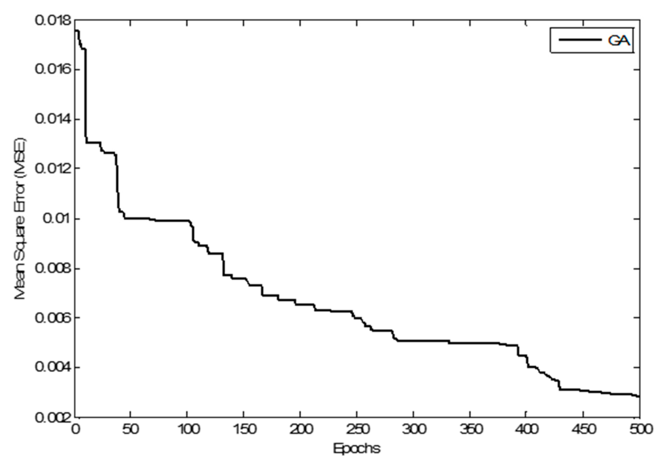
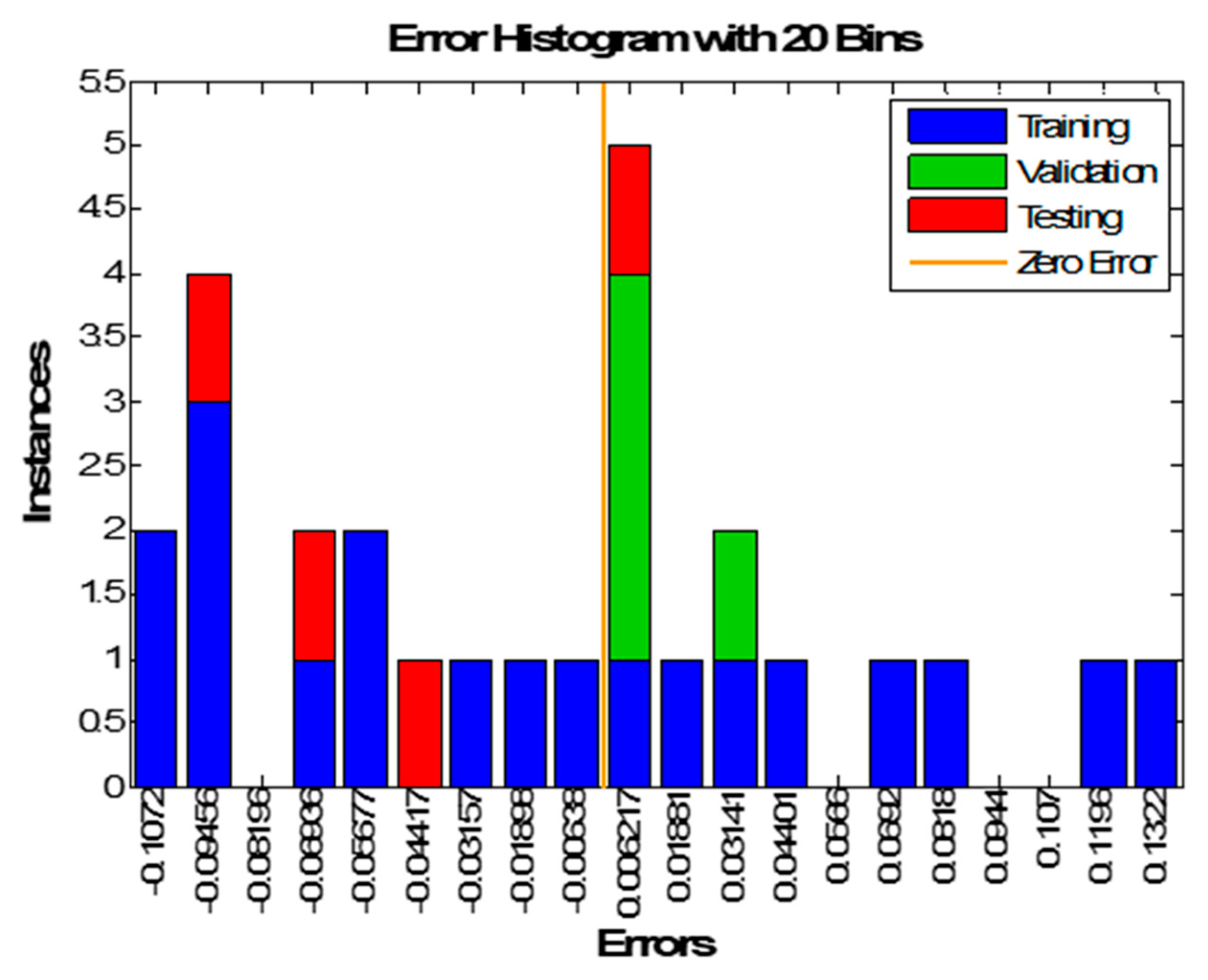
To give a comprehensive view of the GA performance, it is better to construct performance, histogram, and regression plots exactly as with BPNN. Figure 12 shows the training mean square error versus epochs of the ANN-GA model. MSE decreases with epoch until it reaches minimum values, standing for the optimum set of weights and biases. It shows that the ANN-GA has low convergence speed, which is considered one of the limitations of the genetic algorithm.

Figure 13 shows the error histogram of 3-7-1 structure. This error represents the difference between real target and the desired output. The blue, green, and red colors refer to training, validation, and testing errors, respectively. The testing errors for the ANN-GA fall between 0.09456 and 0.006217. 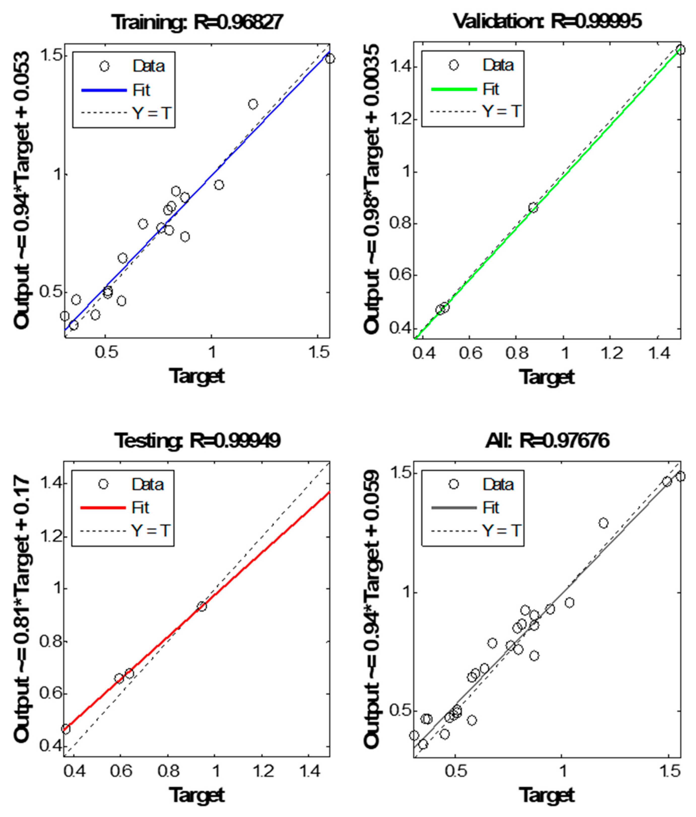To check how much the desired output matches the real target, regression plots are plotted as shown in Figure 14. Obviously, ANN-GA scattering is less than with ANN in training, validation, testing, and all, where All R-values reach around 0.97. The R-values of ANN-GA best models confirmed this issue.

As stated earlier, the mechanism of training of BPNN with gradient descent algorithm is completely different from GA, but the target and task of them in this study are the same. Neural networks apply training with inductivity while GA adopts deductive training in search space, and the assessment of fitness function is required.

4.4. Prediction of Surface Roughness by Hybrid Neural-Gravitational Search Algorithm Model

Table 13. Statistical measures of mean square error of ANN-GSA.

No. of Neurons	MEAN			MEDIAN			STDV			BEST
	Training	Validation	Testing	Training	Validation	Testing	Training	Validation	Testing	Training	Validation	Testing
1	0.019965	0.010207	0.022593	0.0172	7.12 × 10−3	0.019965	0.011205	0.008216	0.013294	0.010484	0.002983	0.005331
2	0.009958	0.00737	0.018378	0.009098	0.007049	0.011891	0.003428	0.004191	0.014087	0.006609	1.84 × 10−3	0.003677
3	1.19 × 10−2	6.55 × 10−3	0.02828	0.010919	5.00 × 10−3	0.01127	8.57 × 10−3	6.86 × 10−3	0.039868	5.26 × 10−3	2.59 × 10−4	5.48 × 10−4
4	7.73 × 10−3	3.52 × 10−3	0.029271	6.99 × 10−3	2.51 × 10−3	1.14 × 10−2	3.62 × 10−3	2.98 × 10−3	5.08 × 10−2	1.99 × 10−3	3.45 × 10−4	2.34 × 10−3
5	6.97 × 10−3	3.36 × 10−3	3.84 × 10−2	5.79 × 10−3	2.24 × 10−3	1.68 × 10−2	3.76 × 10−3	0.00355	0.06747	1.96 × 10−3	1.32 × 10−4	2.01 × 10−3
6	6.97 × 10−3	3.36 × 10−3	0.038443	5.79 × 10−3	2.24 × 10−3	1.68 × 10−2	3.76 × 10−3	3.55 × 10−3	0.06747	1.96 × 10−3	1.32 × 10−4	2.01 × 10−3
7	8.24 × 10−3	3.13 × 10−3	0.022099	6.08 × 10−3	2.20 × 10−3	1.94 × 10−2	5.75 × 10−3	3.02 × 10−3	0.018688	1.71 × 10−3	1.23 × 10−9	2.88 × 10−11
8	7.96 × 10−3	2.58 × 10−3	2.00 × 10−2	7.28 × 10−3	1.71 × 10−3	1.15 × 10−2	5.48 × 10−3	3.19 × 10−3	2.74 × 10−2	5.74 × 10−4	1.68 × 10−8	8.82 × 10−4
9	8.41 × 10−3	3.25 × 10−3	0.025986	5.21 × 10−3	1.25 × 10−3	0.019224	6.80 × 10−3	6.74 × 10−3	2.87 × 10−2	4.14 × 10−4	8.70 × 10−6	1.62 × 10−3
10	9.54 × 10−3	3.74 × 10−3	0.047148	8.56 × 10−3	2.34 × 10−3	0.031088	5.45 × 10−3	5.17 × 10−3	0.076162	2.99 × 10−4	1.33 × 10−4	7.21 × 10−6
11	9.02 × 10−3	3.62 × 10−3	0.028191	7.97 × 10−3	1.35 × 10−3	1.95 × 10−2	5.09 × 10−3	6.05 × 10−3	0.025919	1.45 × 10−3	2.19 × 10−6	1.22 × 10−4
12	8.95 × 10−2	1.13 × 10−1	1.42 × 10−1	6.78 × 10−3	2.51 × 10−3	3.22 × 10−2	8.31 × 10−3	8.68 × 10−3	0.078977	5.95 × 10−4	3.38 × 10−20	1.56 × 10−7
13	1.34 × 10−2	2.24 × 10−3	0.046845	1.25 × 10−2	2.01 × 10−3	2.55 × 10−2	1.04 × 10−2	0.002587	5.57 × 10−2	1.48 × 10−3	8.55 × 10−12	2.23 × 10−12
14	8.40 × 10−2	3.78 × 10−3	0.034314	9.16 × 10−3	1.61 × 10−3	1.86 × 10−2	6.56 × 10−3	6.02 × 10−3	0.042803	4.35 × 10−4	1.04 × 10−17	2.93 × 10−4
15	1.19 × 10−2	1.95 × 10−3	0.042868	8.14 × 10−3	1.13 × 10−3	3.01 × 10−2	9.91 × 10−3	2.37 × 10−3	0.032809	7.88 × 10−4	4.08 × 10−19	1.69 × 10−4
16	1.01 × 10−2	1.24 × 10−3	0.060574	8.81 × 10−3	4.43 × 10−4	2.68 × 10−2	7.05 × 10−3	1.89 × 10−3	8.37 × 10−2	2.32 × 10−3	1.75 × 10−13	2.30 × 10−4
17	7.07 × 10−3	1.39 × 10−3	0.083012	5.79 × 10−3	5.06 × 10−4	4.86 × 10−2	7.53 × 10−3	2.44 × 10−3	8.82 × 10−2	2.71 × 10−4	1.68 × 10−15	7.41 × 10−13
18	1.32 × 10−2	3.35 × 10−3	0.046086	1.14 × 10−2	6.12 × 10−4	3.94 × 10−2	8.01 × 10−3	7.24 × 10−3	0.039601	2.63 × 10−3	7.20 × 10−19	1.03 × 10−6
19	1.03 × 10−2	1.23 × 10−3	0.083768	1.05 × 10−2	8.11 × 10−4	8.28 × 10−2	5.58 × 10−3	1.18 × 10−3	0.069804	2.39 × 10−3	8.75 × 10−10	1.51 × 10−3
20	1.21 × 10−2	3.24 × 10−3	0.069405	1.03 × 10−2	1.03 × 10−3	5.15 × 10−2	8.13 × 10−3	4.96 × 10−3	0.077374	2.74 × 10−3	5.06 × 10−13	8.03 × 10−4
minimum	0.006968	0.001232	0.018378	0.005213	4.43 × 10−4	0.01127	0.003428	0.001178	0.013294	0.000271	3.38 × 10−20	7.41 × 10−13

shows the statistical measures of the mean square error for the training, validation, and testing phases of the ANN-GSA model. The results in Table 13 revealed the high performance of GSA when integrated with ANN. The best model for ANN-GSA of the PVD cutting tool is 3-17-1. This model has 17 hidden neurons and recorded minimum mean square errors of 7.41 × 10⁻¹³.

Table 13 shows the significant effect of hidden neurons that GSA has exploited in addition to its high convergence speed to enhance the performance of ANN. In other words, GSA was able to adopt the increasing of hidden neurons for some network structures to minimize the error between the real target and desired output to as low as possible. In addition to the 3-17-1 network structure, which has been selected as the best model, it can be shown from this table that other network structures also achieved very good results, such as the 3-7-1, 3-8-1, 3-10-1, 3-12-1, 3-13-1, and 3-18-models.

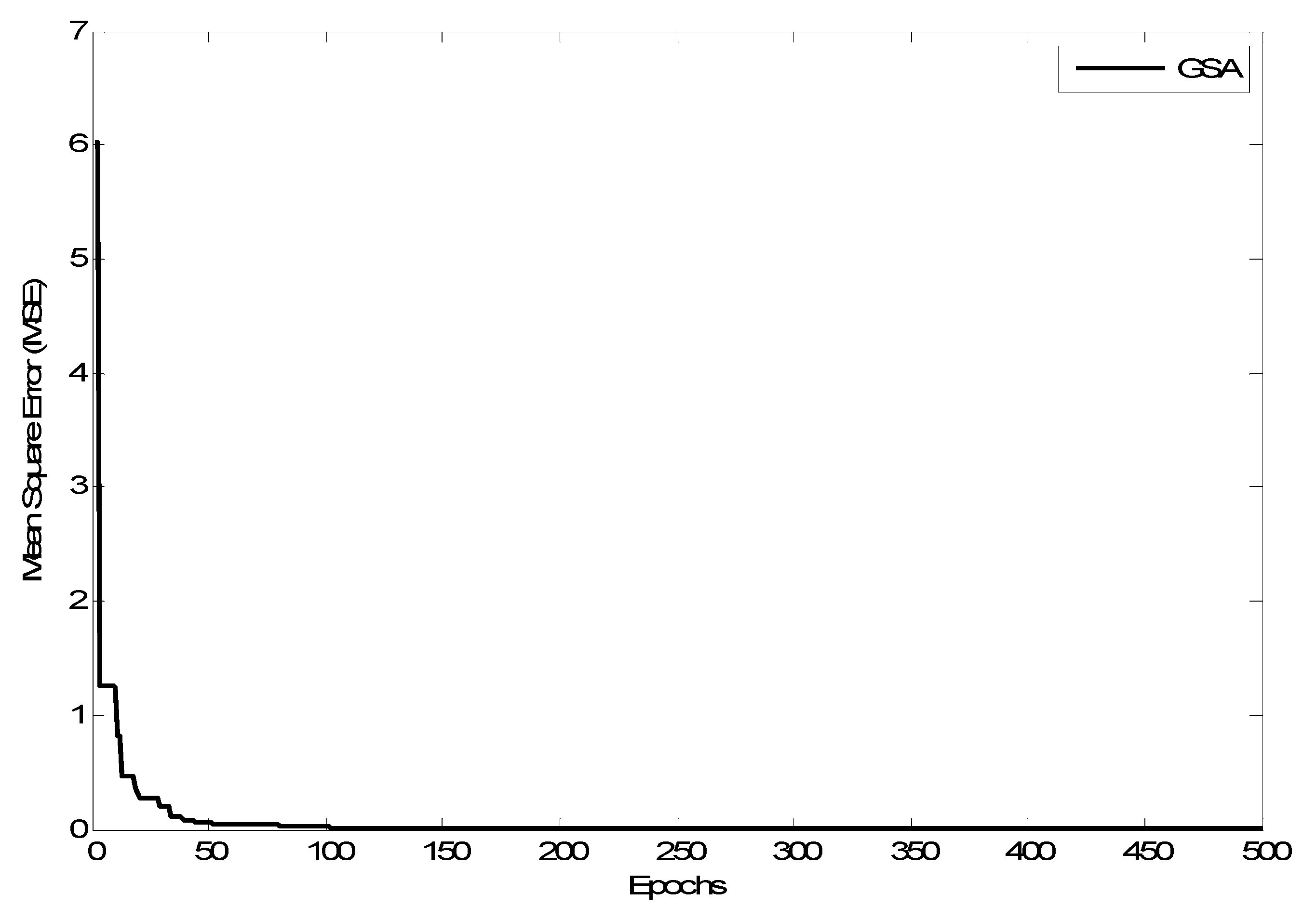
Regarding the mean, median, and standard deviation, they obtained a minimum MSE of 0.018378, 0.01127, and 0.013294, respectively, with ANN-GSA. These values are less than the corresponding ones for ANN and ANN-GA. Figure 15 shows the training mean square error versus epochs ANN-GSA model. The training performance takes like L shape, unlike the GSA algorithm. It continues to steer the solution iteration by iteration toward optimum points to achieve the best weights and biases that keep the network with minimum mean square error.

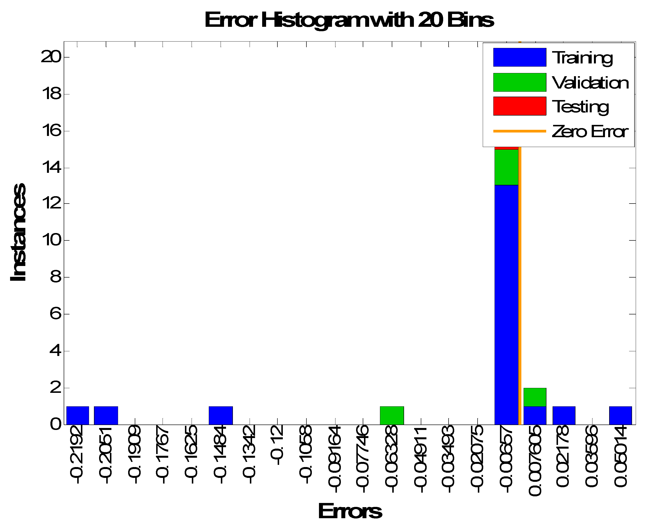
For more verification of the reliability of the developed hybrid model, the training, validation, and testing errors are plotted as histogram plots as shown in Figure 16. The same colors that have been used previously for training, validation, and testing error bars are used here in same sequence. Two differences distinguish Figure 16 from the corresponding ones of other algorithms. The first difference is the testing errors, which are close to the zero line. The second difference is that around 75% of errors centered around the zero line, including most of the training and validation data points and the full testing set. This explains why ANN-GSA got the minimum testing MSE compared with the other algorithms. The testing error of ANN-GSA was 0.00657.

The regression plots are shown in Figure 17. It can be noticed from the regression plots that ANN-GSA has a high R-value, especially in testing where it recorded 1. This issue revealed the effectiveness of GSA in training ANN by maintaining minimum testing error (Figure 16), minimum testing mean square error (Table 13), and finally, high testing R values (Figure 17). The results of performance, histogram, and regression plots seem identical and present a comprehensive view of the capability of ANN-GSA to enhance BPNN performance by providing a best set of weights and biases that make desired output much closer to the real target. These plots were very helpful in clarifying, explaining, and presenting the results in a very good view.

4.5. Performance Comparison of the Developed Neural and Hybrid-Neural Algorithms

As stated earlier, ANN is simply mimicking the task of the brain. It has processing elements known as neurons, and those neurons are interconnected with each other by synaptic weights. BPNN is sometimes trapped in local minima and cannot reach the global solution, especially with a complex problem. The neural network started its weights initialization from a point far from the global point. Therefore, it was necessary to find a solution for this problem by improving the performance of BPNN to achieve a better solution than the existing one.

Recently, there has been a trend toward enhancing the performance of neural networks by integrating them with evolutionary computation (EC). Significant efforts have been made to handle this task to evolve the neural network aspects. It can be noticed that the most commonly applied evolutionary computation techniques share the following similar characteristics:

• Starts with an initial population with a random generation.
• Evaluations of fitness function of each subject (chromosome, particle, or agent).
• Population reproducing based on values of the fitness function.
• If targets have been hit, then stop; otherwise, do steps 2-4 again.

Looking at the flowcharts of GA and GSA, it can be concluded that both of them share common aspects. Firstly, they initialize their population with random generation (weights and biases). Secondly, they evaluate the population by fitness function (MSE). Thirdly, they search for optimum solutions and update the population, and finally, they do not give a guarantee of success.

However, they are also different from each other in some points. For example, GA has crossover and mutation operations not available in GSA. GA population moves as one object because the chromosomes share information. In contrast, in GSA, since each agent can observe the performance of the others, the gravitational force is an information transference tool.

The purpose of this short introduction and simple comparison is to reveal that the performance of those hybrid models will be different from each other. However, the fitness function is the same, though the mechanism of searching for global solution is different. Hence, the results will not be same because those techniques are stochastic not deterministic based.

After training, validation, and testing of all neural and hybrid neural models, the best one of each model has been selected to make a fair performance comparison.

Table 14. Minimum testing mean square error of ANN, ANN-GA, and ANN-GSA models.

Algorithm	Mean	Median	STDV	Best
ANN	0.047803	0.023347	0.043889	0.002219
ANN-GA	0.029546	0.025057	0.02044	0.004
ANN-GSA	0.018378	0.01127	0.013294	7.41 × 10−13
Minimum	0.018378	0.01127	0.013294	7.41 × 10−13

shows the testing mean square errors of ANN, ANN-GA, and ANN-GSA, respectively. The results undoubtedly revealed that ANN-GSA’s performance is the best among the models because it accomplished minimum mean square error in the testing phase.

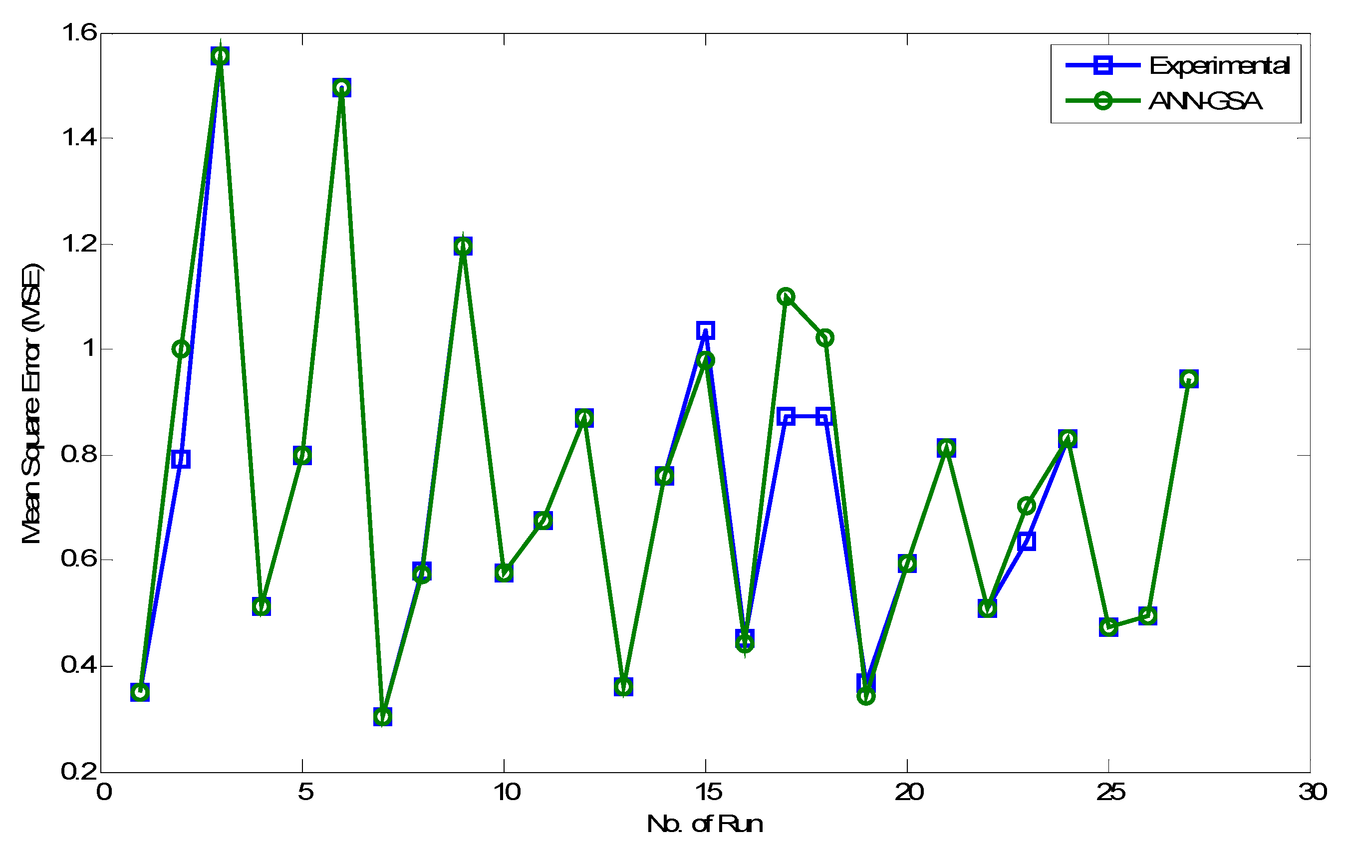
Obviously, the ANN-GSA hybrid model has overcome the performance of other algorithms in all statistical measures. The best model for ANN-GSA is the 3-17-1 network structure, and it consists of 17 hidden neurons and recorded minimum mean square errors of 7.41 × 10⁻¹³. By extracting the predicted values from the best models, Figure 18 is constructed. The impact of GSA in training BPNN is that a very good agreement has been obtained between the target and desired output.

Table 15. Weights and biases of 3-17-1 ANN-GSA hybrid model.

Hidden Neurons	Weights of Input-Hidden Layers			Bias of Input-Hidden Layers	Weights of Hidden-Output Layers	Bias of Hidden-Output Layers
	Cutting Speed (m/min)	Feed Rate (mm/Tooth)	Depth of Cut (mm)
1	0.950647	1.109773	−3.28231	−3.55006	0.138562	−0.21649
2	2.285847	2.443147	1.847223	−2.81363	0.627436
3	−0.72484	0.735741	3.468026	2.665944	−0.35846
4	−2.7085	−1.66507	−1.37738	2.391054	0.269709
5	−0.15831	3.36584	1.014338	1.832393	0.126811
6	2.329043	1.23884	−2.43448	−1.33164	−0.1353
7	−2.57064	0.63113	−2.4486	0.941609	−0.16869
8	−0.83912	2.699705	−2.11733	0.188848	0.190304
9	−2.29716	2.08027	−1.64158	−0.3477	0.228521
10	2.511161	−0.74023	2.527545	0.380805	−0.3167
11	0.997379	−1.97111	2.634426	1.262534	0.781721
12	2.581125	0.675932	2.206369	1.472184	−0.01274
13	−1.80267	2.586812	−1.77669	−1.80348	0.181059
14	0.262186	2.083198	2.3811	2.831749	0.392518
15	2.377391	−2.68754	0.208772	2.637499	0.429414
16	2.086752	−3.02313	0.358296	3.047992	−0.52273
17	−2.412	−2.45436	1.076532	−3.59588	−0.12234

presents the optimum weights and biases for the 3-17-1 model, which is the best model of the ANN-GSA algorithm. It consists of 17 hidden neurons and has 86 weight values, including 18 biases.

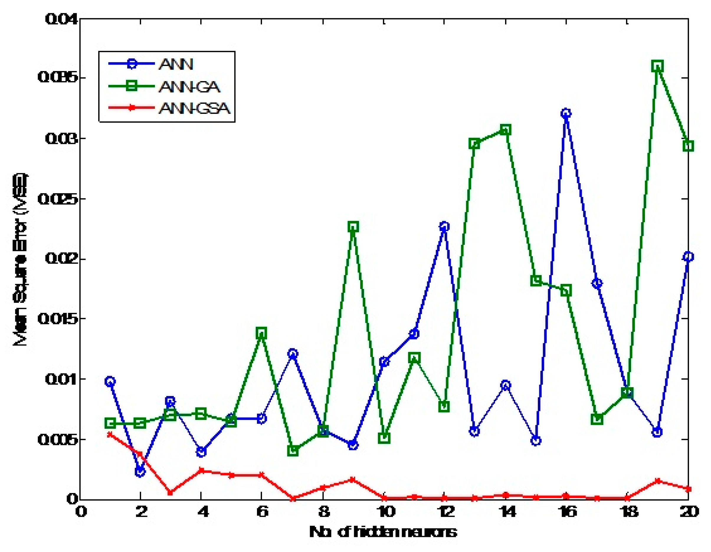
Another important thing that can be added to the discussion to support the findings is plotting the best MSE in testing all algorithms against the number of hidden neurons. Figure 19 shows the effect of hidden neurons on the performance of different algorithms. Figure 19 reveals the random response of ANN and ANN-GA algorithms to increasing the hidden neurons for a PVD coated tool. Their fluctuation and spikes over the number of hidden neurons can be seen. In contrast, the performance of ANN-GSA was very good versus the range of hidden neurons. Consequently, it achieved minimum MSE testing for all hidden neurons except neurons 1, 2, and 9.

Capability and performance of each algorithm, size and quality of data set, network structure, and starting points of initialization of weight and bias are four factors affecting the quality of the achieved result. Consequently, GSA was capable of steering and orienting the solution direction towards the global point regardless of data set nature and starting point for different network structures.

4.6. Statistical Analysis for Evaluation of Artificial Intelligence Algorithms

Statistical analysis of developed artificial intelligence models is one of the critical issues that show whether the obtained results are significant or not. Furthermore, it justifies which AI model is the best and, at the same time, provides the ranking of models based on their significance degree.

Because more than two algorithms have been developed in this study, the Post-Hoc Multiple Comparisons test has been adopted to investigate the performance of the three Artificial intelligence (AI) developed models. According to the conducted literature review, this test has never been used before in milling process statistical analysis or AI models. The analysis of variance or ANOVA is utilized to compare the means of more than two populations. It reveals the effect of independent variables and/or their interaction on the dependent variable(s). ANOVA has found extensive application in psychological research using experimental data. It can also be used in business management, especially in consumer behavior and marketing management related problems [42].

First, the developed algorithms’ results will be tested by a Post-Hoc test to know which is the best algorithm and why. Also, the rank of the developed algorithms is essential to show how these hybrid algorithms could improve the performance of ANN. The best testing results will be used in the analysis because the best testing results represent the best optimum weights and biases of that run among all the other twenty runs.

In this study, three algorithms have been used: ANN, ANN-GA, and ANN-GSA. Rejection of the null hypothesis in ANOVA only tells us that all population means are not equal. Multiple comparisons are used to assess which group means differ from which others once the overall F-test shows that at least one difference exists. Many tests are listed under “Post-Hoc” in SPSS. Tukey HSD (honestly significant difference) test is one of the most conservative and commonly used tests [42]. The one-way ANOVA results, including descriptive statistics, ANOVA, Post-Hoc test, and homogeneous subsets, are shown in

Table 16. One-way ANOVA results.

Descriptive
Algorithms	N	Mean	Std. Deviation	Std. Error
ANN	20	0.01	0.007	0.002
ANN-GA	20	0.01	0.010	0.002
ANN-GSA	20	0.00	0.001	0.000
Total	60	0.01	0.009	0.001
ANOVA
	Sum of Squares	df	Mean Square	F	Sig.
Between Groups	0.002	2	0.001	16.486	0.000
Within Groups	0.003	57	0.000
Total	0.005	59
Post-Hoc Test (Multiple comparisons)
(I) Groups	(J) Groups	Mean Difference (I–J)	Std. Error	Sig.
ANN	ANN-GA	−0.003	0.002	0.318
	ANN-GSA	0.010	0.002	0.000
ANN-GA	ANN	0.003	0.002	0.318
	ANN-GSA	0.013	0.002	0.000
ANN-GSA	ANN	−0.010	0.002	0.000
	ANN-GA	−0.013	0.002	0.000
Homogeneous Subsets
Groups	Subset for Alpha = 0.05
	1		2
ANN-GSA	0.001078
ANN			0.01
ANN-GA			0.01
Sig.	1.000		0.318

.

The null hypothesis in this case is:

H01: 

The average MSE of all four algorithms is the same.

Table 16 shows the ANOVA results. Between groups refer to the variability due to different algorithms that have been applied, the within groups present variability due to random error, and the third row shows the total variability. The F-value is 14.001, and the corresponding p-value is <0.000. Hence, the null hypothesis should be rejected, and all algorithms’ average MSE is not the same. The Post-Hoc test shows the comparison between all the possible pairs (Table 16). Since we have four algorithm pairs for each case study, a total of twelve pairs will likely be mirror images.

The following pairs of algorithms recorded p-values less than 0.05, and this means that the average difference of MSE between them is significant:

• ANN_ANN-GSA (p < 0.000)
• ANN-GA_ANN-GSA (p < 0.000)
• ANN-GSA_ANN (p < 0.000)
• ANN-GSA_ANN-GA (p < 0.000)

The ANN-GSA was superior because it outperformed all other algorithms by achieving p-values less than (0.000) compared with ANN and ANN-GA. This means the difference is significant and GSA’s ability to improve the performance of ANN is better than GA. Furthermore, the mean difference between ANN-GSA and other algorithms is minus. In other words, the average MSE of ANN-GSA is less than others.

The homogeneous subsets (Table 16) show the same results as another form. The algorithms are ranked based on increasing mean value. They have been divided into two homogeneous subsets where ANN-GSA has occupied the first subset with a minimum mean value of (0.001078). In contrast, ANN and ANN-GA have been put in the second subset, which means there is no significant difference between them. To sum up, GSA proved its effectiveness and superiority in enhancing ANN performance.

5. Conclusions

This study has investigated the effects of cutting conditions on the surface roughness of Ti6Al4V alloy during end milling with a PVD coated tool under dry cutting conditions. Taguchi method was adopted with an L27 orthogonal array to generate 27 experimental runs. The backpropagation neural network has been hybridized with a heuristic technique called gravitational search algorithm (GSA) to develop the ANN-GSA hybrid model. Also, BPNN was integrated with a genetic algorithm (GA) to produce an ANN-GA hybrid model. All the developed models were exploited to predict the surface roughness of Ti6Al4V alloy during end milling with a PVD coated tool under dry-cutting conditions. Based on the achieved results, the following conclusions could be drawn:

• The most significant factors affecting machined surface quality are feed rate and cut depth.
• High cutting speed accompanied with low feed rate and depth of cut is the optimum cutting condition that achieves minimum surface roughness.
• One way ANOVA test approved the vitality and effectiveness of GSA compared with BPNN and GA.
• The minimum testing MSE of the ANN-GSA model was 7.41 × 10⁻¹³ which is considerably less than corresponding values of BPNN and ANN-GA.
• The performance of GSA when changing the number of hidden neurons was very good while the response of BPNN and GA was random and obtained many spikes.
• The testing errors were centered on the zero line in the ANN-GSA model, unlike the BPNN and GA algorithms.
• The ANN-GSA algorithm achieved less scattering of data points in training, validation, and testing.
• Very good agreement was achieved between experimental and predicted data points.