Prediction of Tool Shape in Electrical Discharge Machining of EN31 Steel Using Machine Learning Techniques

Abstract

In the electrical discharge machining (EDM) process, especially during the machining of hardened steels, changes in tool shape have been identified as one of the major problems. To understand the aforesaid dilemma, an initiative was undertaken through this experimental study. To assess the distortion in tool shape that occurs during the machining of EN31 tool steel, variations in tool shape were examined by monitoring the roundness of the tooltip before and after machining with a coordinate measuring machine. The change in out-of-roundness of the tooltip varied from 5.65 to 37.8 µm during machining under different experimental conditions. It was revealed that the input current, the pulse on time, and the pulse off time had most significant effect in terms of changes in the out-of-roundness values during machining. Machine learning techniques (decision tree, random forest, generalized linear model, and neural network) were applied for the prediction of changes in tool shape. It was observed that the results predicted by the random forest technique were more convincing. Subsequently, it was gathered from this examination that the usage of the random forest technique for the prediction of changes in tool shape yielded propitious outcomes, with high accuracy (93.67%), correlation (0.97), coefficient of determination (0.94), and mean absolute error (1.65 µm) values. Hence, it was inferred that the random forest technique provided better results in terms of the prediction of tool shape.

1. Introduction

EDM is a type of unconventional machining process that involves the use of thermal erosion as the mechanism of material removal, and the process is primarily utilized in the manufacturing of dies. In EDM, stock from the specimen is removed by means of continuous discharges between two electrodes, i.e., the tool and the work material. It causes the creation of a plasma channel and the temperature reaches the range of 7500–19,000 °C, thereby removing the material from the electrodes via melting and evaporation [1,2,3,4,5]. As the supply of pulsating current is withdrawn, the plasma envelope collapses and the dielectric removes the melted material from the machining site in the form of debris.

The EDM process has many advantages, which include its ability to machine a large range of electrically conductive materials regardless of their hardness, with high accuracy, and without the need for any post machining in the majority cases, among other benefits. However, the EDM process is not free of problems, with associated issues including electrode wear, low material removal during the machining of hard materials and hardened steels, and changes in the profile of the tool during the machining process (especially the materials with high hardness values); these problems can be minimized by using composites that will have lower deformation. The performance of EDM process generally depends upon certain work/tool-related factors, in addition to user-specified factors such as the discharge current, breakdown voltage, gap voltage, pulse on duration, pulse off duration, machining time, duty cycle, polarity, dielectric pressure, etc. The efficiency of the EDM process is evaluated in terms of the Material Removal Rate (MRR), the Surface Roughness (SR), the Tool Wear Rate (TWR), the surface integrity, and the dimensional accuracy of the finished product. The responses have been optimized using different mathematical models and statistical techniques. At present, artificial intelligence (AI) is contributing significantly to all engineering fields. It plays an important role in every industry, especially in the machining industry. The technologies and techniques, in conjunction with AI applications, are being extensively used in machining processes [6].

Jeswani [7] used dimensional analysis to analyze the erosion that occurs in the EDM process. An empirical equation was generated, which related the tool wear with the thermophysical properties of the tool material. The coefficient of correlation for the obtained equation was 0.99, which indicates a very good fit. Tsai and Wang [8] studied various neural networks and neuro-fuzzy (ANFIS) approaches to predict the MRR of different work materials. ANFIS were found to perform better than other techniques in the prediction of MRR, with an error of 16.33%. The process parameters for the EDM process were optimized by Fenggou and Dayong [8] using ANN combined with the use of GA and a node-deleting algorithm. With the application of GA and Back Propagation (BP) algorithms, the training speed of the models was increased significantly. A similar study was conducted by Singh et al. [9] to optimize the process variables for MRR, TWR, SR, taper, and radial overcut in EDM by utilizing Grey Relational Analysis (GRA). The GRA process was simplified via the conversion of a single response from a multi-response parameter. El-Taweel [10] studied the impact of the current, flushing pressure, and pulse on time on the MRR and TWR. These variables were chosen by multi-response optimization using RSM. The RSM predicted the MRR and TWR with 7.2% and 4.74% error rates, respectively.

Sahu et al. [11] detailed the effect of the current, duty factor, dielectric pressure, and pulse time on the MRR and TWR using RSM. Every trial was considered as a decision-making unit and their relative efficiencies were obtained by means of data-envelopment analysis. The results were projected with a maximum error of 4.22%. A semi-empirical model was proposed by Talla et al. [12] to analyze the powder-mixed EDM process. A Principal Component Analysis (PCA)-based GRA technique was applied for the optimization of this analysis. To achieve higher MRR and lower SR values, a set of machining variables was also recommended. Kumar et al. [13] suggested a regression model to estimate the MRR and TWR. The sufficiency of the model was justified by ANOVA. The developed model was successful in predicting MRR and TWR values, with accuracies of 94.65% and 96.91%, respectively. Walia et al. [14] modeled the change in the shape of the Cu-TiC tooltip using Buckingham’s dimensional analysis. The results predicted by the developed model were found to be in agreement with the actual observations as the prediction error varied from +5.89% to −6.91%. El-Bahloul [15] evaluated the performance of an RSM- and ANN-based model and compared it with a model based on fuzzy logic. Coefficient of determination, root mean square error, and absolute average deviation calculations were used for the comparison. The RSM- and ANN-based model was found to be more reliable and accurate. Perez [16] used a fuzzy interference system (FIS) and developed a technological table. The purpose of the technological table was to decide the optimum process parameters for the maximization or minimization of the response according to specific requirements. The results obtained with FIS were compared with the results acquired with RSM and were found to be more accurate. The performance of the harmony search algorithm (HSA) was compared with Taguchi grey relational analysis (TGRA) by Mahalingam et al. [17]. The result obtained with HAS proved to be better, and the prediction error was less than 6%.

Some of the significant contributions of the EDM process to the analysis of different optimization tools and process parameters are presented in

Table 1. Summary of a few key studies used for the analysis of responses [18,19,20,21,22,23,24,25,26,27,28,29,30].

Author	Optimization Tools	Response	Parameters
Laxman and Raj [18]	Taguchi	MRR, TWR, SR	Current, pulse on/off duration, tool lift time
Assarzadeh and Ghoreishi [19]	ANN (BP)	MRR, SR	Current, pulse period, source voltage
Joshi and Pande [20]	FEM, ANN	MRR, TWR, crater geometry	Discharge power, pulse on time, duty factor
Yahya et al. [21]	ANN	MRR	Pulse on/off duration, sparking frequency, gap current
Gopalakannan and Senthilvelan [22]	RSM	MRR, TWR	Current, pulse on duration, pulse off duration
Nikalje et al. [23]	Taguchi method	MRR, TWR	Current, pulse on duration, pulse off duration
Baraskar et al. [24]	RSM, multilinear regression analysis	MRR, SR	Pulse on duration, pulse off duration, current
Das et al. [25]	Artificial bee colony (ABC) algorithm	MRR, SR	Discharge current, pulse off time, pulse on time, voltage
Zhang et al. [26]	FEM	Energy distribution and diameter of plasma	Polarity of workpiece, pulse duration, dielectric pressure
Raja et al. [27]	Firefly algorithm (FA)	Machining time and SR	Current, pulse on duration
Mohanty et al. [28]	Multi-objective particle swarm algorithm	MRR, EWR, SR, radial overcut	Voltage, current, pulse on duration, duty factor, dielectric pressure
Payal et al. [29]	Taguchi-fuzzy	MRR, SR	Discharge current, pulse on duration, voltage, dielectric fluid, tool lift time
Pandey and Gautam [30]	Genetic algorithm	Hole taper, hole circularity, hole dilation	Pulse on/off duration, discharge current, flushing pressure

.

It is recognized from the survey of the literature that a large amount of research has been undertaken in relation to the investigation of the prediction of MRR, EWR, and SR. Applications of different statistical and modeling techniques (such as fuzzy logic, GA, GRA, ANN, RSM, FEM, etc.) have been used for the evaluation of these responses. From the literature, it was also found that the pulse on time, pulse off time, input current, and flushing pressure are some of the most important parameters in terms of their effects on the EDM process [31,32,33,34]. In the EDM process, heat is produced at both electrodes (i.e., at the tool and the workpiece). This heat removes the material from both the tool and the workpiece. The removal of material from the tool also causes changes in the shape of tool, which, in turn, is transferred to the workpiece because, in EDM, the workpiece is a replica of the tool. The same point is highlighted in this study, which can be very helpful in industrial applications, specifically in relation to the reduction in the rejection rate of manufactured parts due to changes in the shape of the tool. However, there are very few sources available in the literature [34] that discuss the influence of process variables in terms of changes in tool shape during the EDM process, and this work is one of the first works that attempts to develop a proper relationship, using machine learning techniques, between the parameters that most significantly affect the tool shape. EN31 steel was used as the work material in this study as it is abundantly used in the manufacturing of dies, which is the major application area of EDM. The hardened EN31 steel was used as the work material because it would cause the tool to encounter more challenges in terms of maintaining its shape during machining. A round-shaped tool was used as it allowed the change in tool shape to be easily measured and assessed by measuring the change in roundness of tool tip before and after machining. Through this work, an initiative was taken to use machine learning techniques (decision tree, random forest, generalized linear model, and neural network) for the prediction of change in the shape of the tool. These techniques are very precise and are rarely used for the assessment of machining processes. Moreover, the assessment of variation in the shape of the tool using the aforementioned prediction techniques has not yet been explored.

The paper is structured as follows: Section 2 focuses on the details of the workpiece, the choice of process parameters, and the recording of experimental observations, and includes a brief overview of the machine learning techniques used, as well as the methodology followed during the study of feature importance. In Section 3, a quick summary of the parameters used to assess the applied techniques is given. Section 4 enumerates the results in detail, followed by a comparison and discussion. Finally, the conclusions of the current work are presented in Section 5.

2. Experimental Procedures

In order to analyze the change or variation in the shape of the tool, experiments were performed on a die-sinking EDM machine (EIL-Pune, India). The copper tool was utilized for the machining of the hardened EN31 workpiece. The analysis of the tool shape was conducted using a coordinate measuring machine (CMM) (Hexagon-Noida, India). The entire process is detailed below.

2.1. Workpiece and Tool Material

Hardened EN31 tool steel was used as the work material in this study. Copper was chosen as a tool material due to its excellent thermal and electrical properties. The workpiece material was cut into a specimen size of 15 × 15 × 6 mm³. The heat treatment of the work material was performed to ensure that the machining of difficult work material was conducted under standard working conditions. After heat treatment, the hardness of the workpiece material increased from 20 HRC to 56 HRC. The parameters used for the heat treatment of the workpiece are presented in

Table 2. Heat treatment parameters.

Hardening	Parameter	Level	Tempering	Parameter	Level
	Hardening temperature	850 °C		Tempering temperature	260 °C
	Soaking time	20 min		Soaking time	1 h
	Heating rate	600 °C/h		Heating rate	600 °C/h

. The chemical composition of heat-treated EN31 tool steel was also determined with an optical emission spectrometer (Foundry Master, Oxford Instruments; Uedem, Germany) before experimentation. The composition of EN31 tool steel after heat treatment is summarized in

Table 3. EN31 steel composition.

Carbon	Silicon	Manganese	Chromium	Sulphur	Phosphorous	Iron
1.09	0.32	0.62	1.14	0.026	0.035	Rest

.

2.2. Selection of Process Parameters and Data Generation

EN31 tool steel workpieces were machined using die-sinking EDM (Reliable, 55300). Commercially available EDM oil, with a flashpoint of 90 °C and specific gravity of 0.77, was used as the dielectric medium for all of the experiments. Depending on the capabilities of the machine and pilot experiments that were conducted, five controllable parameters, including the input current (I_p), voltage gap (V_g), flushing pressure (P), and pulse on time (T_on), as well as the pulse off time (T_off), were selected. The ranges for these parameters were decided based on the capability of the EDM machine. Their combinations were achieved by varying each factor and keeping the other factors constant. Here, one parameter was initially varied as per the values given in

Table 4. Experimental parameters.

Peak current, Ip	3, 4, 5, 6, 7, 8, 9, 10 and 11 A
Gap voltage, Vg	40, 45, 50, 55, 60, 65, 70, 75 and 80 V
Ton	100, 150, 200, 250, 300, 350, 400, 450 and 500 μs
Toff	10, 15, 20, 25, 30, 40, 45 and 50 μs
Dielectric pressure, P	12, 13, 14, 15, 16, 17, 18, 19 and 20 kgf/cm2
Electrode polarity	−ive
Work material polarity	+ive
Dielectric	EDM oil
Flushing	Side flushing
Work material	EN31 steel (Hardened)
Hardness of work material	56 HRC

. For the other parameters, during the same stage, the central value was selected (for example, when Ip was varied from 3 to 11 A in step 1 A, the Vg values were 60 V, Ton 300 μs, and Toff 30 μs, and the flushing pressure was 16 kgf/cm²). The experimental parameters used in the present work are shown in Table 4.

By varying the process parameters within the selected range, there were 262 experiments conducted in this study. The duration of machining was fixed at 30 min for each experiment. It was previously established that higher tool hardness leads to lower wear rates [35,36]. During the EDM process, due to edge wear and rounding of the tool edge (as shown in Figure 1), a change in the shape of the tool profile was observed. To estimate the change in the tool shape during machining, variations in the roundness of the tool were measured before and after the electric discharge machining process. The out-of-roundness was measured using a coordinate measuring machine (Accurate, Spectra 564 model) shown in Figure 2 Accusoft plus software was used for the analysis of data. Twelve points were randomly marked on the circumference of the tooltip, as shown in Figure 2. On the basis of these markings, an ideal profile of the round shape of the tool was generated by the software. After that, the variations in the dimensions of the marked points from the ideal profile were determined, and were designated as the change in roundness, i.e., in the shape of the tool. The procedure was adopted to measure the roundness of the tool tip before and after the EDM process. The difference in these two measurements was taken to be the change in the tool shape in terms of the change in the roundness units.

The out-of-roundness value was recorded before and after machining for each tooltip. The difference between the two observations of roundness values for the tooltip (denoted as a change in out-of-roundness) was taken to be the response to the analysis of the change in shape of the tool (as shown in

Table 5. Out-of-roundness of the tool tip before and after machining (I_p = 9 A, V_g = 50 V, T_on = 200 µs, T_off = 20 µs, P = 18 kgf/cm²).

Out-of-Roundness of Tool Tip before EDM = 0.0126 mm				Out-of-Roundness of Tool Tip after EDM = 0.0417 mm
								Out-of-roundness during EDM = 0.0291 mm
	Mea	Nom	Dev		Mea	Nom	Dev
X	247.3966	247.3966	0.0000	X	250.2975	250.2975	0.0000
Y	136.8872	136.8872	0.0000	Y	152.5679	152.5679	0.0000
Z	133.3678	133.3678	0.0000	Z	133.9986	133.9986	0.0000
DIAM	9.9556	9.9556	0.0000	DIAM	9.9816	9.9816	0.0000
CIRLTY	0.0432	0.0000	0.0432	CIRLTY	0.0839	0.0000	0.0839
SIGMA	0.0126	0.0000	0.0126	SIGMA	0.0417	0.0000	0.0417

). Figure 3 presents the out-of-roundness results for various combinations of process parameters.

2.3. Machine Learning Techniques

Machine learning techniques are more accurate than statistical techniques, especially when the association between the response and process parameters is likely to be non-linear. These techniques can recognize and model the complicated non-linear connections between the process variables and the response [37,38]. These techniques work on the dataset and are very rarely used in the assessment of machining processes. A brief description of these techniques is given below:

Decision Tree (rpart): In a decision tree, the training data are organized in already-predefined classes. Each entry is designated by a discrete label. This classification is performed either through logical models or using the experience of experts. In this technique, the attributes are segregated into classes depending on their features. The main advantage of the decision tree is that, in this technique, the data are classified, using logical models, with greater accuracy [39]. This method is an extended version of the C4.5 classification algorithms detailed by Quinlan [40].

Generalized Linear Model (glm): A linear model is a statistical model that follows normal distributions and conducts regression, single stratum analysis of variance, and analysis of covariance. On the other hand, the generalized linear model is an extension of the linear model that allows data to be non-normally distributed. Here, the linear regression is generalized by linking the linear model to the response variable using a link function.

Random Forest (rf): Random forest is a regression technique used for the prediction of a response. It takes an input vector that consists of variables that have been inspected for a particular training dataset and leads to the development of many regression trees. The random forest technique calculates an average of these results. It further diversifies the trees by growing the trees with the use of different training data subsets, thereby avoiding the correlation between the different trees. During the growth of a tree, it utilizes the best feature by means of random selection from evidential features that are available in the overall set of input features. Consequently, it decreases the correlation between the trees by decreasing the strength of each tree, and thus avoids generalization errors. Samples that are not used for the training purpose become members of another subset known as the out-of-bag subset, which is used for the performance evaluation. Thus, the random forest technique calculates the generalization error without considering the text data externally.

Neural Network (neuralnet): In neural networks, the function of the human brain is represented mathematically. Neural networks are taught via experiments for the execution of non-linear mappings. The characterization of neural networks is performed through the structure of the network and the training algorithm. Artificial neurons or nodes are the processing elements of neural networks. Synapses are the links that connect the neurons. Every synapse is defined by a synaptic weight. Neurons are positioned in the layers. Neurons in each layer function in parallel. In the first layer, the non-processed information is entered into the network. This layer does not execute any computations. The input layer is followed by the hidden layers. The number of hidden layers may vary from zero to many, and the performance of neural networks depends on their number. There is no algorithm that is available to determine the number of hidden layers required for the solution of a particular problem [41]. Thus, the specific problem decides the architecture of the neural network and it must be kept simple. The last layer is known as the output layer, which executes the calculations, and the output of this layer is the output of the whole network. The activities of the hidden layers and the weights between the hidden layers and output layer decide the behavior of the output layer [42].

2.4. Methodology

Figure 4 shows the methodology adopted in the present study. In the first phase, the EN31 tool steel was cut into work material of the required dimensions. Hardening and tempering of the workpiece were undertaken, and a hardness of 56 HRC was attained. The roundness of the tool was measured to observe the tool shape before EDM using a coordinate measuring machine (CMM) during phase 2. In the third phase, die-sinking EDM of the hardened EN31 tool steel workpiece material was performed with the copper tool. The out-of-roundness of the tool was measured again after EDM. The difference between the two measurements was represented as the out-of-roundness of the tool during machining, as shown in Table 4, and this corresponds to the fourth phase. The importance of each process parameter was measured in the fifth phase to ensure that the prediction was efficient and accurate. In phase six, machine learning techniques, specifically the decision tree, random forest, generalized linear model, and neural network techniques (

Table 6. Machine learning techniques.

Techniques	Method	Package	Tuning Parameter and Values
Decision tree	Rpart	Rpart	Min Split = 20, Max Depth = 30, Min Bucket = 7
Random forest	Rf	Random Forest	mtry = 500, sampling = bagging
Generalized linear model	Glm	Glm	None
Neural network	Neuralnet	Neuralnet	hlayers = 10, MaxNWts = 10,000, maxit = 100

), were used and tested on the hyperparameters. A hyperparameter is a parameter whose value is used to control the learning process. In the decision tree technique, the Max Depth can be described as the length of the longest path from the tree root to a leaf. The root node is considered to have a depth of 0. The Max Depth value cannot exceed 30 on a 32-bit machine. In the decision tree technique, the Min Split specifies the minimum number of samples required to split an internal node. The minimum number of observations that must exist in a node in order for a split to be attempted. The minimum number of observations in any terminal node is called Min Bucket. In random forest technique, the sampling is done by means of the bagging algorithm. This algorithm offers the advantage of allowing many weak learners to combine their efforts in order to outdo a single strong learner. In the random forest technique, there are two ways to find the optimal mtry value: Apply a similar procedure such that random forest is run 10 times. The optimal number of predictors selected for the split is chosen, for which the out of bag error rate stabilizes and reaches its minimum. In the neural network, during training part, the network’s weights are changed with the training algorithm. The training algorithm searches for such a set of weight matrices that, when used in the network, should optimistically map any input to a correct output. In this study, training and testing was repeated for different values of key network parameters such as the number of hidden layers and number of neurons in each layer. The final model and weights of neural network were decided after carrying out a sufficient number of iterations. These techniques were trained to utilize the results obtained from the conducted experiments. These techniques are accessible in R open-source software, which is licensed under GNU GPL. The concepts of correlation, coefficient of determination, mean absolute error, and accuracy were applied to evaluate the efficacy of the applied techniques. The robustness measurement of the predictive methods was verified by K-fold validation. In the last phase, the obtained results were analyzed and conclusions were drawn.

2.5. Parameter Importance Using Regularized Trees

To improve the performance of the model, feature selection was performed using the Regularized Random Forest (RRF) model. It was found that all of the features were below the cut-off score, so no feature was dropped. This process screened the significant features that would have increased the model’s performance. The existing Regularized Random Forest (RRF) model was applied for the feature selection task because it operates by applying a single ensemble as opposed to multiple ensembles. In this case, if the features had values of more than one with the same consistent information gain, then any one feature was chosen randomly. In the RRF model, the node impurity is calculated by means of the Gini index [43]. When applied in this study, parameters with higher node purity were assigned a higher rank. Based on the node purity, the ranking of the variables gauged by RRF is shown in

Table 7. Importance of each process parameter.

	Ip	Ton	Ton	P	Vg
Score	70.46	9.65	5.84	0.23	0.06
Ranking	1	2	3	4	5

. According to the RRF, I_p was the most influential factor for the shape of the tool. The V_g parameter was recognized as the least important for the selected dataset.

3. Performance Evaluation of Machine Learning Techniques

The performance of a technique can be evaluated through different criteria and the suitability of a given technique depends upon its specific application. In the present study, the correlation (r), coefficient of determination (R²), mean absolute error (MAE), accuracy, and K-fold cross-validation were selected for the assessment of the applied techniques. These criteria were preferred based on a previously conducted review of the literature [44]. These evaluation criteria are briefly discussed below.

Correlation (r) is a statistical technique that shows the relationship between actual and predicted values. The correlation coefficient lies between +1 and −1, where values closer to +1 indicate a stronger relationship, and values closer to −1 indicate a weaker relationship, between the actual and predicted responses. It is defined using Equation (1).

$$r=\frac{{\sum }_{i=1}^n\left(e_i-\overline{e}\right)\left(p_i-\overline{p}\right)}{{\sum }_{i=1}^n{\left(e_i-e\right)}^2{\sum }_{i=1}^n{\left(p_i-\overline{p}\right)}^2}$$

(1)

where ‘$p_i$’ is the predicted value, ‘$e_i$’ is the experimental value, ‘$\overline{p}$’ is the mean of all predicted values, ‘$\overline{e}$’ is the mean of all observed values, and ‘n’ is the number of instances.

The coefficient of determination (R²) represents the closeness of the data to the fitted regression line. R² illustrates the proportion of variance of the dependent variable elucidated by the regression model. The value of R² varies between 0 and 1, where a value of 1 indicates the perfect regression model and a value of 0 indicates the total failure of the model. The R² is calculated as given below:

$$R^2= r \times r$$

(2)

The mean absolute error (MAE) is the measure of the difference between the predicted value and the observed value. The MAE is calculated using the following equation:

$$\mathrm{MAE}=\frac{{\sum }_{i=1}^{n }\left|p_i-e_i\right|}{n}$$

(3)

where e_i is the experimental value and p_i is the predicted value.

The percentage deviation of the predicted value from the observed value, with acceptable error, is referred to as accuracy, and is given below as Equation (4).

$$\mathrm{Accuracy}=\frac{100}{n}{{\displaystyle \sum }}_{i=1}^n{Z}_i$$

(4)

$$Z_i=\{\begin{array}{c}1 if abs \left(p_i-e_i\right)\le err\\ 0 otherwise\end{array}$$

where, ‘$e_i$’ is the experimental value, ‘$p_i$’ is the predicted value, and ‘err’ is the acceptable error, which was taken to be ±0.04 µm for the present work. The acceptable error was based on the evaluation of the data that were used for prediction.

The stability of a model can be evaluated by K-fold cross-validation. It is measured by assessing the generalization of the model to an independent dataset. In a predictive model, the model is trained using a known dataset and the testing of the model is conducted against an unknown dataset to check the ability of the model to work under real conditions. In this technique, a dataset is divided into k subsamples of the same size. (k − 1) subsamples are applied for the training of the data and the remaining subsample is used for validation of the method. This process is repeated k number of times with every subsample acting as validation data once. The final evaluation is obtained by averaging the results obtained from the k number of cycles. This method is superior to the random sub-sampling method as, when using this method, all observations are utilized for training and validation purposes at least once.

4. Results and Discussion

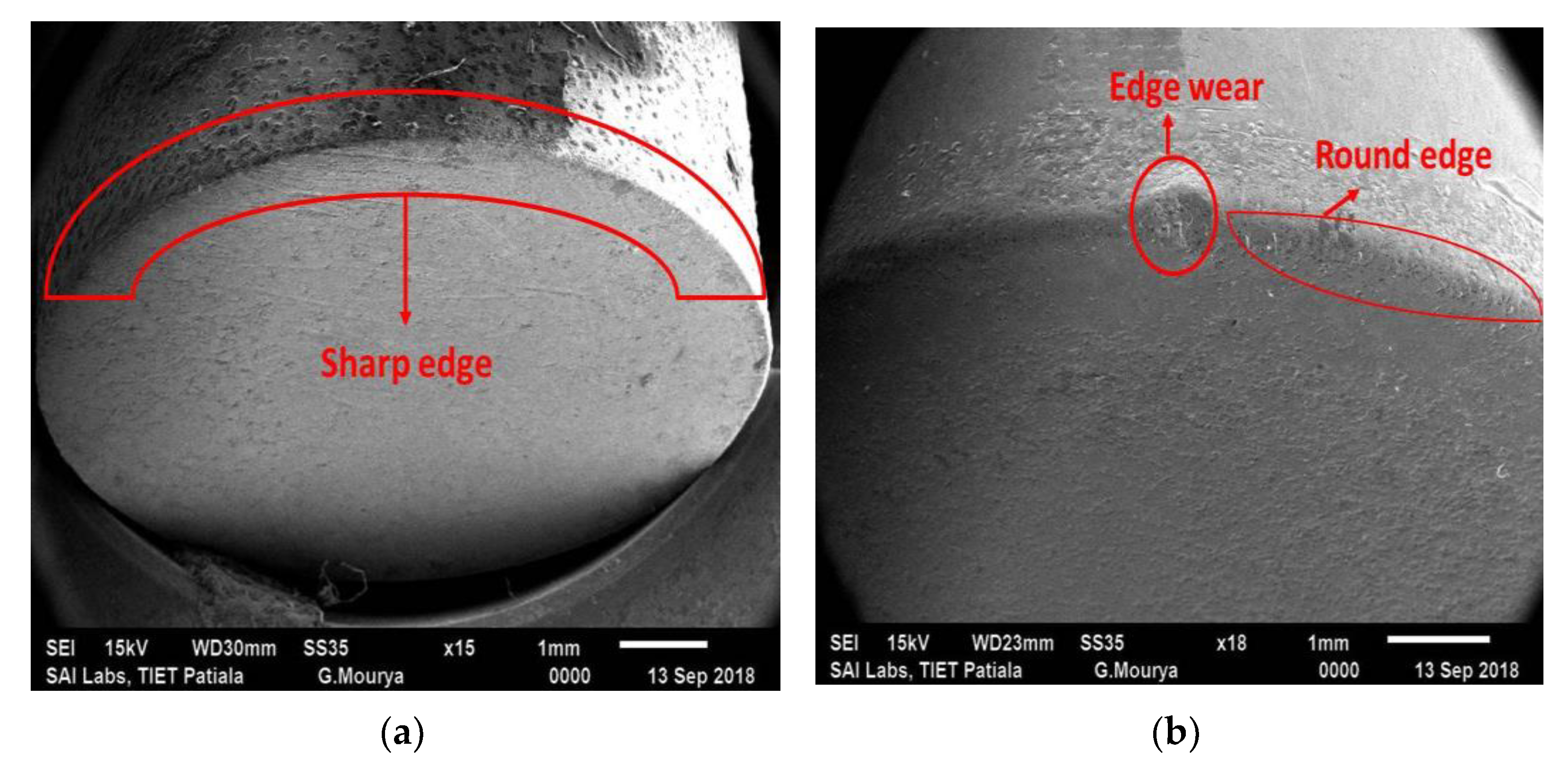
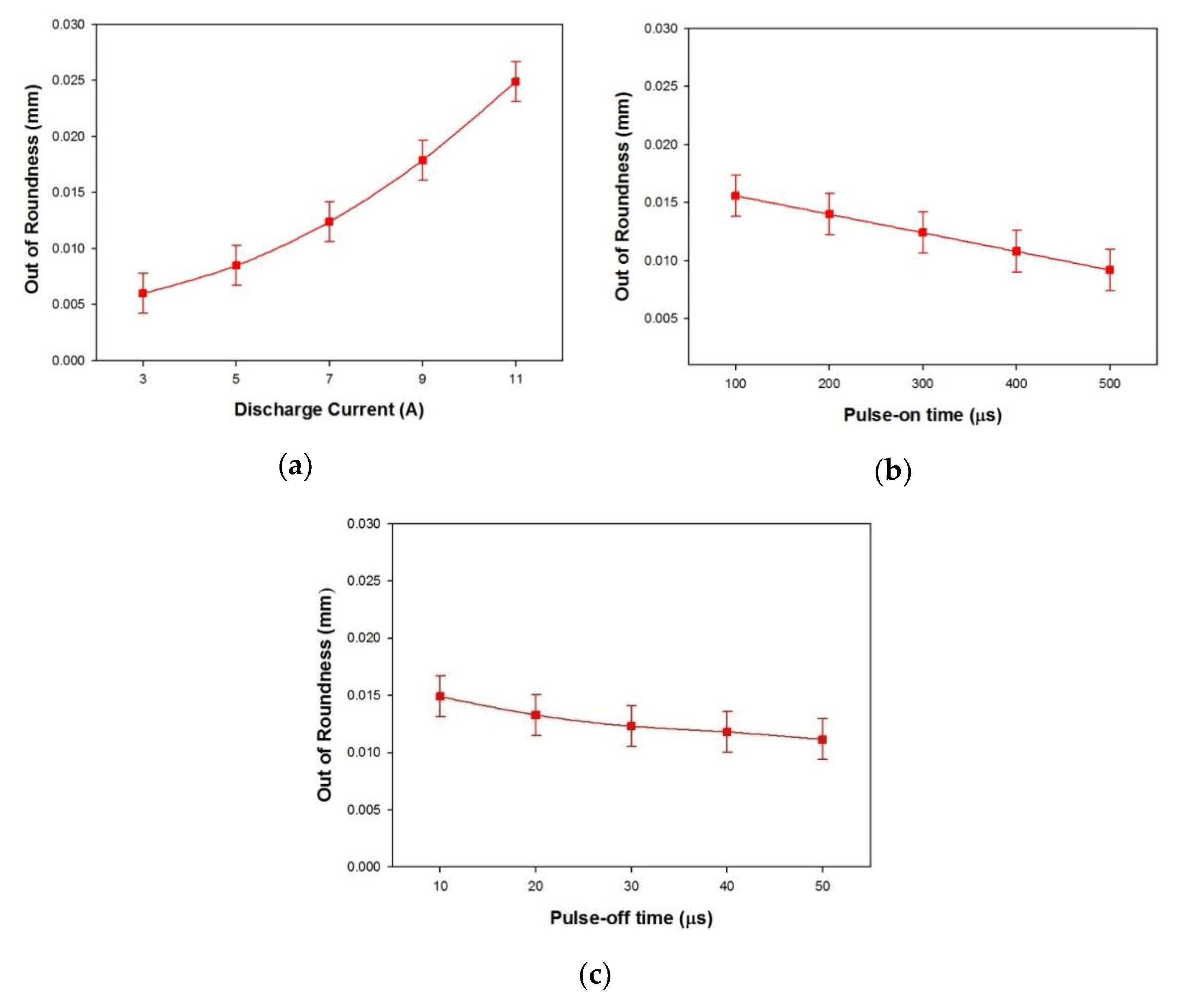
In EDM, the replica of the tool is produced on the work material. In the EDM process, the spark that causes the erosion on the workpiece surface is generated from the surface of the tool. This spark originates at the point where the distance between the tool and the surface of the workpiece is at its smallest. After one spark, the location of the minimum distance changes. In effect, the minimum distance phenomenon causes the spark to travel across the surface of the tool. As a result, the replica of the tool is depicted on the workpiece. Therefore, if any change or variation occurs on the tool during the EDM process, the final geometry of the work material may undergo variation away from the desired geometry. In this study, the tool shape was analyzed by evaluating the variation in the out-of-roundness of the tool before and after machining.

Figure 5 shows the effect of I_p, T_on and T_off on the out-of-roundness values. An increase in out-of-roundness was noticed with the increment in the input current, as presented in Figure 5a. The electrical discharge column in the inter electrode led to the removal of the material from the workpiece as well as leading to the decomposition of the electrode material. With the increase in supplied current, higher energy was generated in the inter-electrode gap, which led to an increase in the distortion of tool material [45].

The effect of increases in pulse on time (T_on) values on out-of-roundness for the EDM process is shown in Figure 5b. It is evident from the figure that the out-of-roundness tended to decrease with the increment in the pulse on time. As the T_on increased, the diameter of the discharge column also tended to increase, which led to the decrement in the energy density of the electrical discharge [46,47,48].

Figure 5c represents the effect of pulse off time (T_off) on out-of-roundness. With an increment in T_off, there was a rapid decrease in the out-of-roundness of the electrode. Lower T_off values led to increases in the frequency of sparks, which tended to generate more heat. Furthermore, the heat generated in the tool electrode consequently had no time to dissipate. This heat was thus entrapped in the tool electrode, which led to increases in the distortion of the shape of the tool electrode.

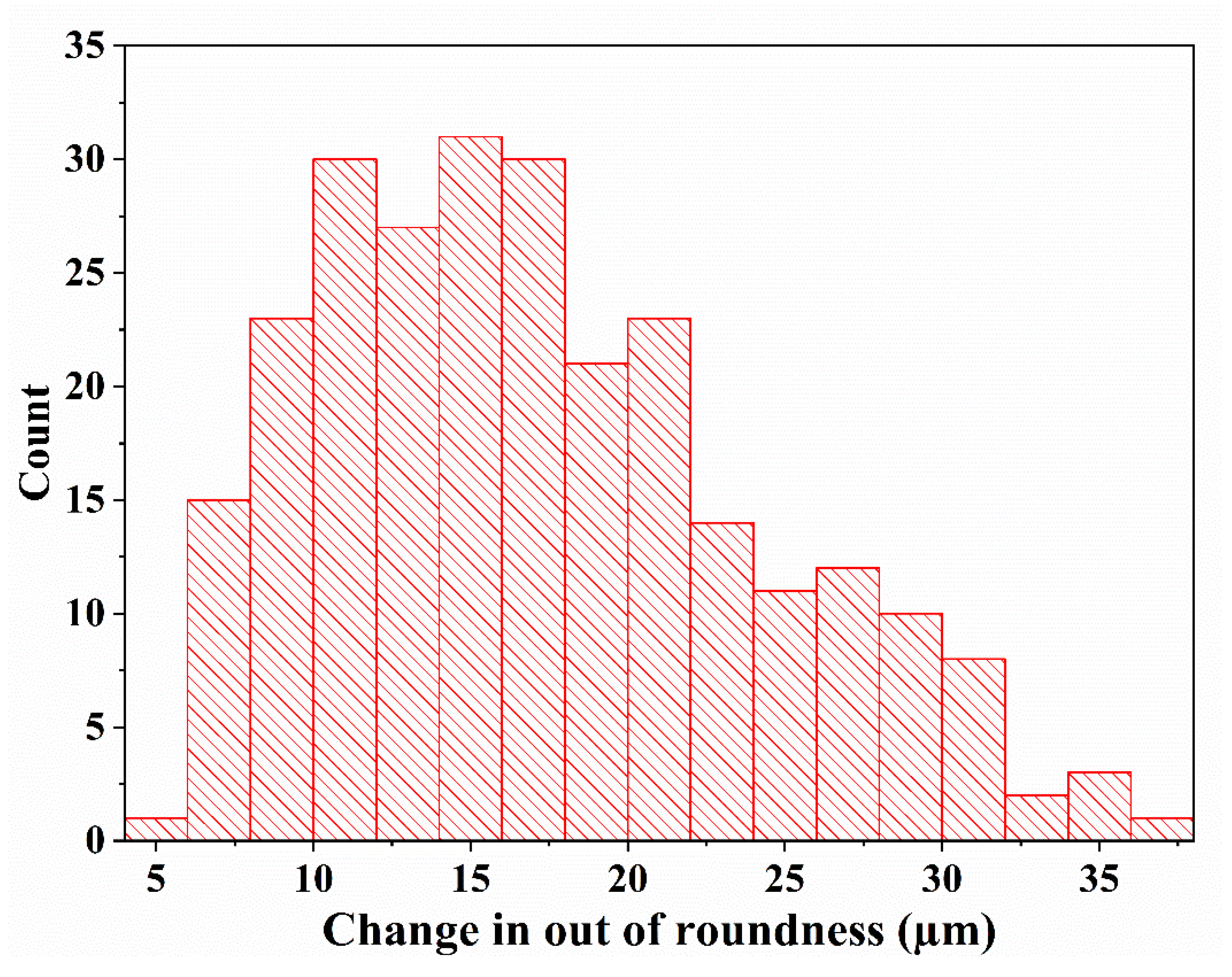
The measured response data for different trials are shown in Figure 3. The data obtained for the changes in out-of-roundness of the copper tooltip were analyzed. 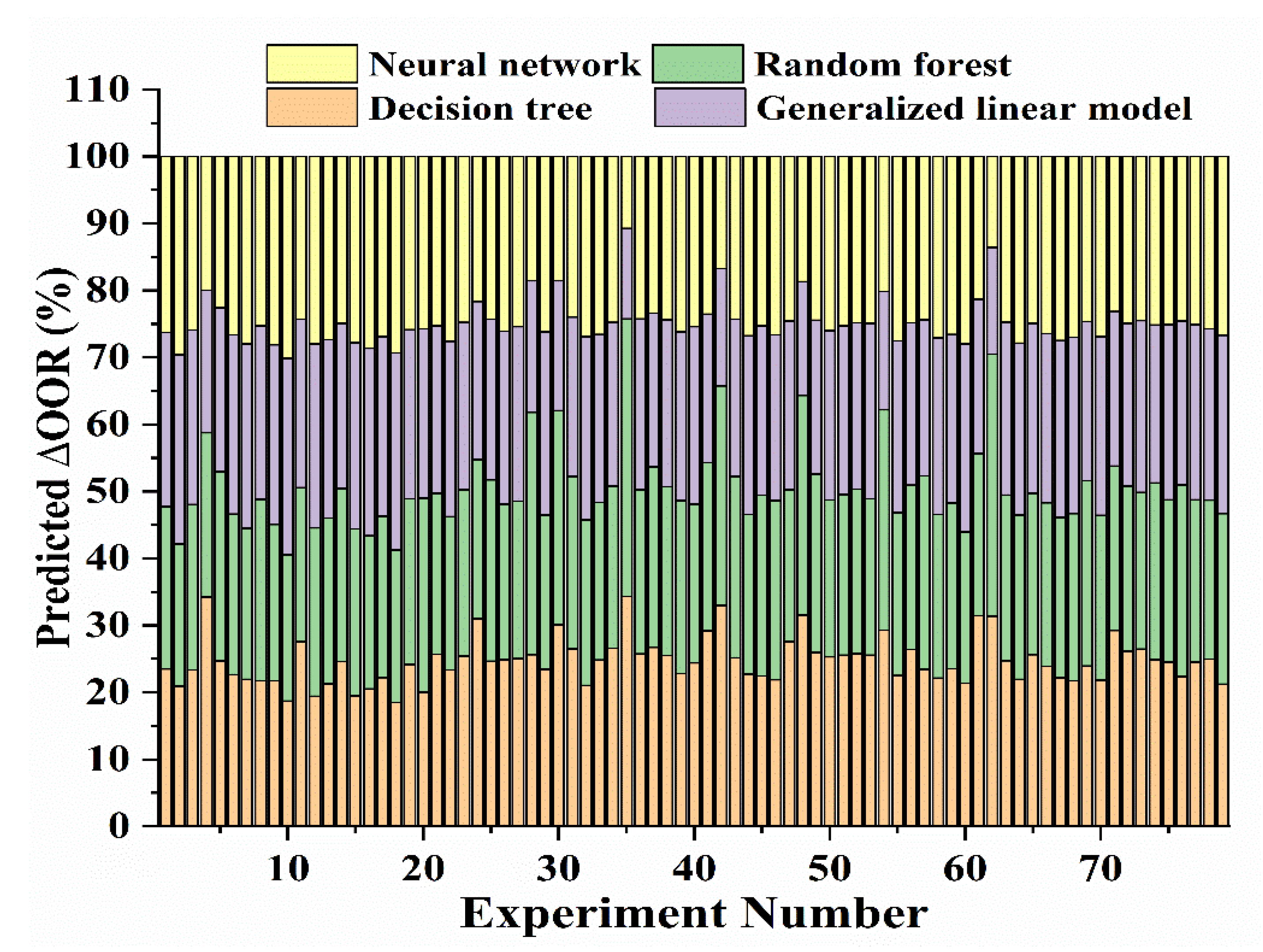Large variations in the changes in out-of-roundness values for the tooltip were recorded (from 37.08 µm for I_p = 10 A, V_g = 70 V, T_on = 200 µs, T_off = 20 µs, P = 18 kgf/cm² to 5.66 µm for I_p = 3 A, V_g = 60 V, T_on = 300 µs, T_off = 30 µs, P = 17 kgf/cm²). The average change in out-of-roundness was found to be 17.25 µm. To predict the change in the out-of-roundness of the tooltip, four machine learning techniques were applied to the data obtained from the experiments. The data were utilized for training and testing purposes in the ratios of 70 and 30, respectively. The simulation for out-of-roundness was performed using these data and the results obtained using the applied techniques are shown in

Table 8. Comparison of the performance of machine learning techniques in terms of the prediction of out-of-roundness.

Technique	Correlation	R2	MAE	Accuracy %
Decision tree	0.88	0.78	2.26	83.54
Random forest	0.97	0.93	1.65	93.67
Generalized linear model	0.92	0.85	2.08	88.61
Neural network	0.92	0.85	2.09	91.14

against the pre-selected criteria, namely the correlation, coefficient of determination, mean absolute error, and accuracy. It was observed that when applying an error band of ±0.04 micron, 93.67% of the data were found to be in the significant zone for the random forest technique. A comparison of the techniques used for the prediction of the response is presented in Table 8.

Equation (1) was applied for the calculation of correlation. It can be observed from Table 8 that the random forest technique provided the best correlation, with a value of 0.97, whereas the decision tree has the lowest correlation, of 0.88, for the prediction of out-of-roundness. This means that the random forest technique provided the strongest relationship between the actual and predicted values obtained from both the experimentation and modeling processes. The R² was calculated using Equation (2) and the values for each technique are shown in Table 8. It was found that the random forest technique has the highest R² value, i.e., 0.93. Higher R² values indicate that the data are closely bonded to the fitted regression line and have a very small proportionate error in terms of the estimation of out-of-roundness. It can thus be concluded that higher R² values are related to better goodness of fit in the model. In the decision tree technique, the R² value was 0.78, which was the lowest value out of all of the techniques that were used in this study. Therefore, the random forest technique provided the best goodness of fit in relation to the response.

The MAE was determined using Equation (3) and is shown in Table 8. For the better performance of a prediction model, the MAE value obtained via a particular technique should be the least. It can be observed from Table 8 that the random forest technique estimated the response (out-of-roundness) with the lowest MAE value, i.e., 1.65 µm, whereas the decision tree technique estimated the response with the largest MAE value, i.e., 2.26 µm) for the selected dataset. Therefore, it can be concluded that the model developed by the random forest technique predicted the response with the minimum error margin. Equation (4) was utilized to determine the accuracy of the model with an acceptable error margin of ±0.04 µm. The accuracy of the measurement results for the four techniques are shown in Table 8. It can be observed that the random forest technique provided the highest accuracy—of 93.67%—in the prediction of out-of-roundness, whereas the decision tree estimated the same parameter with an accuracy of 83.54%.

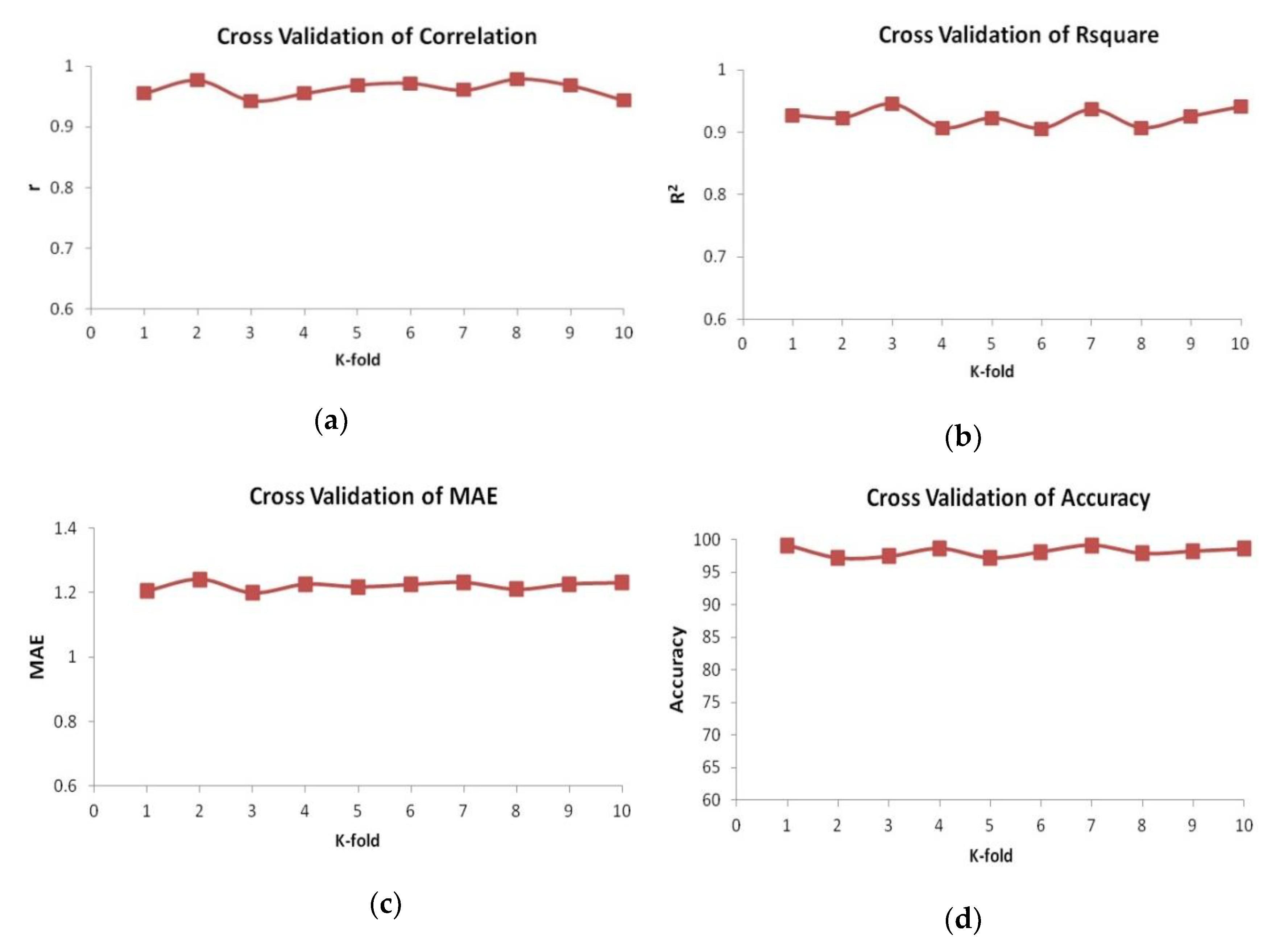
Based on the abovementioned results, as well as the information shown in Table 8 and Figure 6, it can be concluded that, for the prediction of the response (for the selected range of process variables), the random forest technique provided very good results. A 10-fold cross-validation process was applied for the assessment of the robustness of the random forest technique. Figure 7 shows the 10-fold cross-validation of the random forest technique for correlation, R², MAE, and accuracy. The cross-validation results illustrated the consistent performance of the technique. 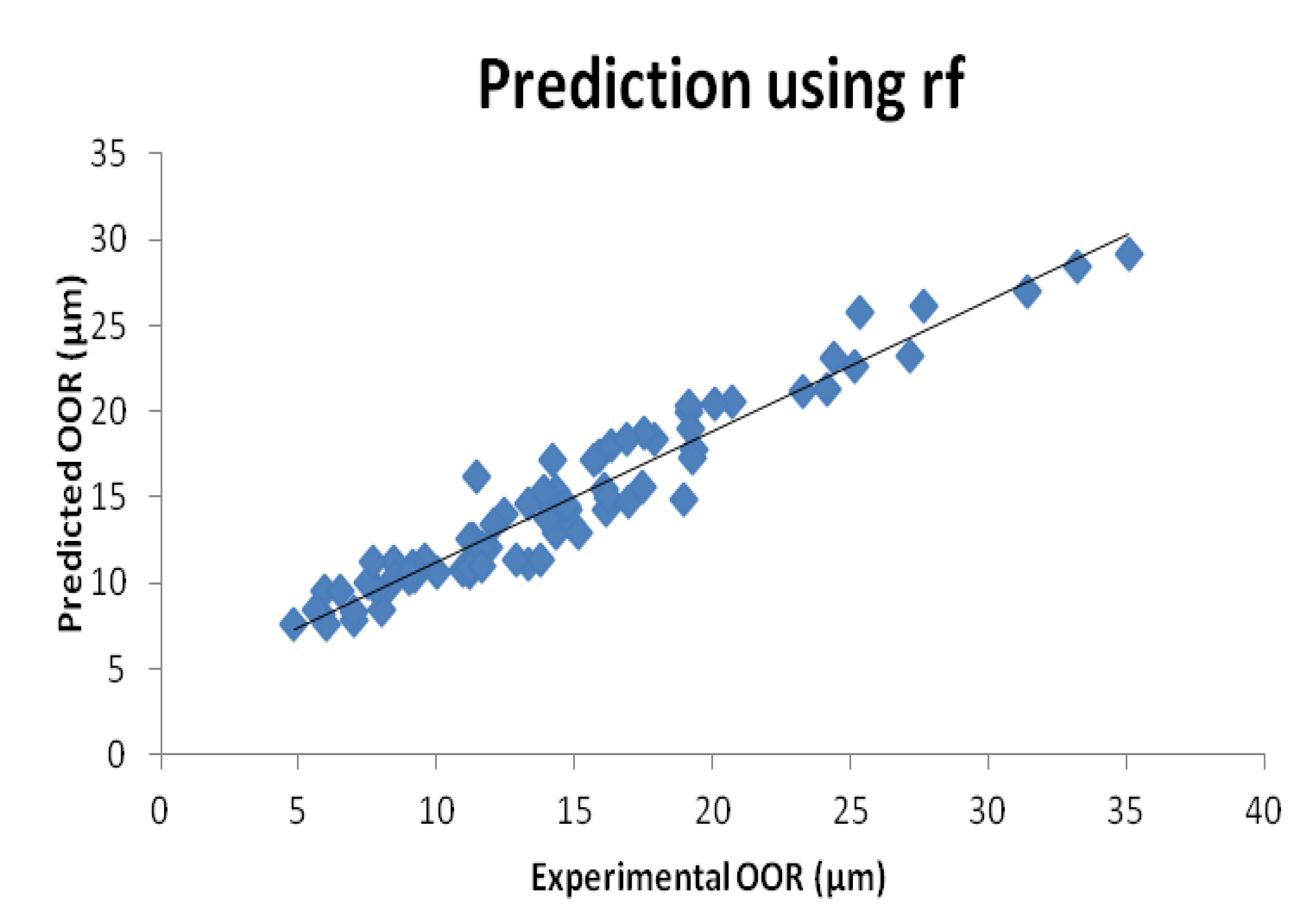Figure 8 highlights the plot between the actual values and the predicted values for the response, i.e., the out-of-roundness values obtained when testing the dataset using the random forest technique. It can be observed from the plot that there are no obvious patterns or unusual structures within the response. Moreover, most of the data are on the linear regression line or in its vicinity. This means that the model developed using the random forest technique is adequate and the closeness of the data points to the mean line highlights the accuracy with which the model can predict the response.

5. Conclusions

In this study, the change in the shape of the tool was recognized as a one of the major aspects of the evaluation of the performance of an EDM process. A coordinate measuring machine was used to measure the change in the shape of the copper tool by analyzing the variation in the out-of-roundness of the tooltip, before and after machining, during the machining process of EN31 tool steel. Four machine learning techniques, namely the decision tree, neural network, generalized linear model, and random forest techniques, were employed to predict the change in the shape of the copper tool. The findings of this work led to the following conclusions:

• It was revealed that I_p, T_on and T_off have most significant effect in terms of changes in out-of-roundness during machining.
• The variation in tool shape was assessed and found to be in the range of 5.66–37.08 µm. Further, for the conducted experimental work, the average variation in terms of changes in tool shape was observed to be 17.25 µm.
• The discharge current was identified as the most influential parameter (70.46%), followed by the pulse on time (9.65%), pulse off time (5.84%), dielectric pressure (0.23%), and gap voltage (0.06%).
• Among the applied machine learning techniques, the random forest technique proved to be the most effective for predicting the response, as it provided the highest correlation (0.97), coefficient of determination (0.93), and accuracy (93.67%), while simultaneously having the smallest mean absolute error (1.65 µm). The decision tree technique had the lowest correlation (0.91), accuracy (83.54%), and coefficient of determination (0.83), whereas it predicted the response with the maximum error of 2.26 µm.
• Ten-fold cross-validation, with the varying of training and testing parameters, revealed that the random forest technique had very high stability and robustness.
• In future studies, the outcome of the current work can be implemented in industrial scenarios with tool electrodes of different shapes, and also under hybrid EDM machining conditions such as ultrasonically assisted EDM processes, cryogenically assisted EDM processes, etc.