Experimental Investigations and Pareto Optimization of Fiber Laser Cutting Process of Ti6Al4V

Abstract

In the current study, laser cutting of Ti6Al4V was accomplished using Taguchi’s L₉ orthogonal array (OA). Laser power, cutting speed, and gas pressure were selected as input process parameters, whereas surface roughness (SR), kerf width, dross height, and material removal rate (MRR) were considered as output variables. The effects of input variables were analyzed through the analysis of variance (ANOVA), main effect plots, residual plots, and contour plots. A heat transfer search algorithm was used to optimize the parameters for the single objective function including higher MRR, minimum SR, minimum dross, and minimum kerf. A multi-objective heat transfer search algorithm was used to create non-dominant optimal Pareto points, giving unique optimal solutions with the corresponding input parameters. For better understanding and ease of selection of input parameters in industry and by scientists, a Pareto graph (2D and 3D graph) is generated from the Pareto points.

1. Introduction

Titanium and its alloys have a good strength-to-weight ratio that is retained even at elevated temperatures [1,2,3]. They have outstanding corrosion resistance and erosion resistance, owing to which there is a wide variety of applications for these alloys in the domain of aerospace engineering, the chemical and petrochemical industries, the pharmaceutical and food processing sector, and offshore and marine engineering [2]. Ti6Al4V is one of the most widely used alloys of titanium, especially in the aerospace industry. It has a better corrosion resistance compared to materials such as stainless steel and cobalt alloys. They are highly resistant to fatigue and have a satisfactory tensile strength at higher temperatures [3].

The ever-increasing manufacturing competitiveness in the present scenario makes the adoption of newer machining technologies more desirable. Challenges such as achieving higher accuracy, better surface finish, increased production rate, and enhanced product life with minimum impacts on the environment, machine operators, and society are of great importance. Additionally, machining hard materials such as Ti6Al4V also requires intelligent machining strategies. Despite their advantageous properties, machining Ti6Al4V alloy can be challenging due to its low thermal conductivity, high reflectivity, and tendency to form an oxide layer. In addition, the high viscosity of Ti6Al4V molten material, and the formation of a brittle heat-affected zone present challenges [1]. Conventional machining of Ti6Al4V exhibits poor machinability, such as unwanted rapid tool wear, poor surface finish, chatter and vibration, etc. [4,5,6]. The Fiber Laser Cutting process is one of the methods that can be used to effectively machine titanium alloys [7,8,9]. A fiber laser is a solid-state laser in which the laser is generated by a laser generator (laser generator is equipped with the optical fiber doped with rare earth elements), and irradiates the specimen [10]. A high-power focused laser is the primary source of heating, causing rapid heating, melting, evaporation, and ablation of the material. Laser beam cutting is the most highly preferable machining process for cutting complex-shaped geometries. This is mainly due to the absence of tool wear, since it is a non-contact machining process. In recent years, mature and efficient high-power fiber laser has been evolving, and the application of fiber lasers has also been increasing in almost all industries [8]. High-power lasers have good laser properties due to their advantageous characteristics. Conventional lasers like CO₂ and Nd-Yag lasers, used for cutting metals, are being replaced by fiber laser cutting to a large extent [9]. Fiber lasers have characteristics like shorter wavelength, good focus ability, and superior beam product parameters, as well as smaller focused diameter, high output power with good beam quality, high operating efficiency, and minimal floor equipment [8,9,10].

In fiber lasers, ytterbium (Yb) is used as the laser generation element. Laser is generated in the laser generation unit, and this is transferred from the generation unit to the machining zone via fiber optics. The resulting laser beam is not focused, so a focused beam is created with the help of focus lenses. The focused beam is then used to irradiate the work material through a nozzle. Thereby, this focused high-density laser is used as the main heat source, and it will start to cause the heating, melting and evaporation of the surface of the work material. At same time, high-pressure assist gas is supplied from the same nozzle, which is collinear to the laser beam. This high-pressure gas helps to exclude the molten material from the machining zone, and realize the cutting of the work material.

Since dimensional and geometric accuracy and the surface quality of the finished product depend primarily on the process parameters, their optimization is of great importance in any machining process [11,12,13,14]. The fiber laser cutting process consists of multiple input parameters and output responses. During machining, it is desirable to achieve an optimal level of all output responses at a single level of input machining variables. One approach to finding a solution for multi-objective optimization problems is to convert multiple objectives into a single-objective optimization problem [15,16,17]. A non-dominated set of solutions, also known as a Pareto front, provides unique solutions. Researchers have developed various efficient advanced optimization techniques that have been shown to be effective in optimizing process parameters for different machining processes. Heat transfer search (HTS) is one such algorithm, and has been found to be easily implemented [18]. The HTS algorithm has been found to be useful for solving complex problems by finding globally optimal solutions [19].

Kratky et al. [20] studied the fiber laser cutting of AZ31 with a 1.5 KW fiber laser source to understand the different merits and demerits of the fiber laser with respect to conventional laser sources. Different applications of fiber lasers, such as remote cutting and welding, have been investigated, and these applications were compared with the different laser sources. The authors concluded that fiber were superior to other laser sources in terms of cost, speed of operation, energy consumption and production rate. J. Powell and A. F. H. Kaplan [21] performed a direct comparison of fiber laser cutting machines and CO₂ laser cutting machines. A comparison of the fiber laser and CO₂ laser source was carried out, and it was found that the CO₂ laser cutting speed was one-third that of the fiber laser cutting speed. They recommended fiber laser for continuous and mass production. In another study, performed by Robert Sołtysiak et al. [22], a comparison of fiber laser and CO₂ laser was performed with respect to the functional properties and cut quality of the cut edge for 6-mm-thick S235JR steel. Characterization of the cut specimens showed high accuracy, low surface roughness value, and good repeatability for both sources. However, the fiber laser exhibited higher functional properties, frequency of service, and efficiency compared to that of CO₂ laser source. B. El Aoud et al. [23] studied the performance of laser cutting of Ti6Al4V with laser power, gas pressure, and cutting speed as the input process parameters, while HAZ and the kerf quality of the cut edge were the output variables. HAZ was observed to be increased with increased laser power, was it decreased with increasing values of gas pressure and cutting speed. Kerf width increased with increasing values of power and gas pressure, while it decreased with an increase in speed. An optimal combination of process parameters was observed at a cutting speed of 2400 mm/min, gas pressure of 2 bars, and laser power of 1 kW. Attia Boudjemline et al. [24] performed experiments using a CO₂ laser source for Ti6Al4V with a thickness of 5 mm, with cutting speed and gas pressure as the machining variables. The cutting speed showed a significant effect for controlling the surface roughness of cut specimens while gas pressure did not show any significant effect. Multiple linear regression analysis and ANOVA were performed to validate the model and there was good agreement between the experimental results and the proposed model. L.D. Scintilla et al. [9] analyzed the effect of cutting speed and gas pressure for fiber laser cutting of Ti6Al4V. They concluded that the selection of machining parameters played a major role in achieving better machining quality. Scintilla and Tricarico [25] investigated the fiber laser cutting process using Nd-Yag and CO₂ laser sources to better understand the effects of cutting speed and assist gas pressure on the cutting quality. Higher cutting speed was achieved in fiber laser cutting, along with a lower SR value. Leonardo Daniele Scintilla and Luigi Tricarico [26] performed experiments using a continuous-mode fiber laser cutting process on aluminum, titanium, and magnesium materials. All experiments were performed using 2 kW laser power while varying the cutting speed from 10 m/min to 30 m/min and using a range of assist gas pressures from 0.3 to 0.6 MPa. They aimed to identify the effect of cutting speed and gas pressure on the cut quality. It was observed that dross and SR increased with increasing speed at 0.3 MPa pressure for titanium. Manjoth et al. [27] used Al7075-TiB₂ as the work material for fiber laser cutting. Taguchi’s L₉ orthogonal array (OA) was used with standoff distance, cutting speed, and gas pressure as the input variables. SR, MRR, and dimensional accuracy were examined. For SR, cutting speed was observed to be the most significant parameter. For MRR, gas pressure and dimensional error, standoff distance was found to be the most influential factor.

At elevated temperatures, titanium alloys tend to react with oxygen and nitrogen. Proper selection of laser cutting process parameters is essential for obtaining good cut quality and for the prevention of hard and brittle martensite formation, as well as nitride and oxide phases when using nitrogen gas as an assist gas [28]. Previous studies have shown that the proper control of machining variables can eliminate or minimize the oxidation effect of laser cutting of Ti6Al4V [29,30]. An increase in the cutting speed significantly decreases the HAZ. An increase in cutting speed rapidly rejects the molten metal in front of the cutting kerf. This gives a very short time for heat conduction. Thus, HAZ decreases with increases in speed due to the shorter exposure time [31]. In a study conducted by Anderson et al. [32], a smooth cut surface was obtained along with negligible HAZ during laser cutting of Ti6Al4V using nitrogen as an assist gas. Poshyananda et al. [28] studied the fiber laser cutting of Ti6Al4V sheet with nitrogen as an assist gas. Their results revealed that the higher cutting speed resulting in smaller HAZ and higher productivity, with enhanced quality of laser cutting. HAZ can be decreased by increasing the cutting speed. However, an increase in laser power has no significant effect on HAZ. Their results also revealed that a far smaller HAZ effect was found during fiber laser cutting, and that this could be easily eliminated through polishing. B. Yilbas et al. [33] examined the effect of laser cutting of titanium alloy. The use of nitrogen as an assist gas resulted in shallow HAZ because of the low thermal diffusivity of titanium alloy. They also concluded that the use of nitrogen resulted in the formation of TiN_x in the cutting section, which in turn increased the brittleness of the recast layer. André Reck et al. [34] examined the effect of laser cutting of Ti6Al4V and the effect of mechanical post-processing. They revealed that optimized parametric settings of laser cutting could significantly eliminate the HAZ. They also analyzed HAZ and found that it did not play a significant role in fatigue failure. SR was found to be more dominant with respect to fatigue failure. Nevertheless, HAZ was entirely removed simply by means of mechanical polishing. Very thin HAZ was obtained during fiber laser cutting as compared to CO₂ and Nd-YAG laser cutting [9]. This is because fiber laser cutting has a high-brightness beam and moves faster, meaning that the material receives very little heat. These past studies show that the proper control of laser cutting process parameters, the use of nitrogen as an assist gas, fiber laser cutting, and mechanical post-processing can significantly eliminate HAZ [28,29,30,31,32,33,34,35,36].

On the basis of the previous literature, it can be seen that fiber laser cutting has not been properly explored with respect to the multi-objective optimization of the machining variables of the fiber laser cutting process. Furthermore, to the best of our knowledge, multi-objective optimization using the HTS algorithm for the fiber laser cutting process parameters of Ti6Al4V has not yet been reported. On the basis of the previous literature, laser power, cutting speed, and gas pressure were selected as the input process parameters, while surface roughness, kerf width, dross height, and material removal rate were considered as output variables in the current investigation. Taguchi’s experimental design, which consists of three levels (L₉ OA), was used to statistically evaluate the effect of input parameters on the analyzed output parameters. Analyses of output responses and the effects of input variables on output responses were carried out with the help of ANOVA, main effect plots, residual plots, and contour plots. Simultaneous optimization of output responses was carried out using the HTS algorithm and mathematical models generated on the basis of the regression analysis. A multi-objective heat transfer search algorithm was used to create non-dominant optimal Pareto points, giving unique optimal solutions with the corresponding input parameters. Finally, a validation study was conducted to verify the results obtained from the algorithm.

2. Materials and Methods

A prime fiber laser cutting machine made by Sahajanand technology was used to perform the experiments on Ti6Al4V.

Table 1. Chemical composition of Ti6Al4V [37].

Element	Al	V	Fe	O	C	N	H	Ti
Weight %	5.86	3.94	0.134	0.100	0.017	0.008	0.00198	Balance

shows the chemical composition of Ti6Al4V. The yield strength, ultimate tensile strength, and hardness values of the selected Ti6Al4V alloy were 955 MPa, 990 MPa, and 320 HV, respectively. Machining specimens of dimensions 30 mm × 30 mm × 3 mm were cut using the fiber laser process. A 3 kW laser source was used to conduct the experiments. In order to supply the assist gas (nitrogen as assist gas), a converging nozzle with an outlet diameter of 2 mm was used. Laser power, cutting speed, and gas pressure were selected as the input process parameters, while surface roughness, kerf width, dross height, and material removal rate were considered as the output variables for this investigation. The input parameters, along with their ranges, were selected on the basis of previous literature and preliminary experimental trials.

Table 2. Fiber laser cutting process parameters.

Process Parameter	Level 1	Level 2	Level 3
Laser Power (W)	2000	2500	3000
Cutting Speed (m/min)	3	4	5
Gas pressure (bar)	8	12	16
Cut focus (mm)	4
Gas	N2
Standoff distance (mm)	0.5
Nozzle diameter (mm)	2
Focal length (mm)	150
Wavelength (µm)	1.07
Mode of Operation	Continous laser
Output Fiber core diameter (µm)	50
Type of Nozzle	Converging

shows Taguchi’s three-level L₉ orthogonal arrays for the three factors that were used to perform the experiments. Table 2 also shows the constant parameters of fiber laser cutting used in the current study. Taguchi’s method has many advantages, such as a reduction in the number of trails, which in turn reduces the cost, time, and resources required during the operations. Taguchi’s method enables many process parameters to be considered, and their effects on selected responses of the process to be analyzed. Figure 1 shows the measurement techniques for the selected response variables of the current study.

Surface roughness is a key parameter that defines the quality of the cut edge. The surface roughness was determined using the Surftest SJ-410 model (Mitutoyo, Ahmedabad, India). An enlarged view of the SR measurement is shown in Figure 1a. The arithmetic average roughness (R_a) value was measured from cut specimens in the current study. R_a is the arithmetic mean of the peaks and valleys of the surface from the centerline or mean line. The cutoff length λ_c was selected as 0.8 mm and the evaluation length was selected as 15 mm during the measurement. Kerf is the amount (width) of material removed from the material during the cutting process. Kerf width measurement was performed using the BX53 microscope (Olympus, Gandhinagar, India). Figure 1b shows the schematic of the kerf measurement. Dross refers to the molten material that is not excluded from the machining zone by gas flow that re-solidifies at the bottom part of the specimen. Dross measurement was performed with help of trinocular microscope MSZ-TR (Magnus, Gandhinagar, India), as shown in Figure 1c. The material removal rate was calculated as the ratio of the weight of the removed specimen to the machining time. In order to achieve higher productivity, MRR must be higher. MRR was measured in g/s, as per Equation (1):

$$MRR=\frac{\mathrm{weight}\mathrm{of}\mathrm{the}\mathrm{removed}\mathrm{material}}{\mathrm{machining}\mathrm{time}}$$

(1)

3. Results and Discussion

3.1. Regression Equations

Table 3. Taguchi’s Design of Experiment (DOE) with the measured values of output responses.

Run	Power (W)	Speed (m/min)	Gas Pressure (bar)	SR (µm)	Kerf Width (µm)	Dross (mm)	MRR (g/s)
1	2000	3	8	8.46	341.75	0.260	2.1924
2	2000	4	12	9.16	337.54	0.280	2.3958
3	2000	5	16	8.92	343.43	0.267	2.6124
4	2500	3	12	9.64	349.32	0.290	2.1680
5	2500	4	16	8.52	351.85	0.265	2.6097
6	2500	5	8	6.83	330.81	0.210	2.8877
7	3000	3	16	9.92	364.48	0.297	2.1248
8	3000	4	8	7.56	337.54	0.250	2.5475
9	3000	5	12	8.78	346.80	0.270	2.7273

shows the measured values of response variables such as SR, kerf width, dross measurement, and MRR with respect to the input machining variables. SR value was observed in the range of 6.83 µm, as a minimum, to 9.92 µm as a maximum on the basis of the nine experimental trials. Similarly, kerf width in the range of 330.81 µm, as a minimum, to 364.48 µm as a maximum, dross value in the range of 0.210 mm, as a minimum, to 0.297 mm as a maximum, and MRR value in the range of 2.1248 g/s, as a minimum, to 2.8877 g/s as a maximum were measured. For the analysis of these measured responses, the statistical software Minitab (Version V17, Gandhinagar, India) was used. Mathematical relations were obtained for each response variable with respect to the machining parameters by using regression analysis. The regression equations for SR, kerf width, dross and MRR are as shown in Equations (2)–(5), respectively:

$$SR=8.96-0.000096·x_1-0.583·x_2+0.1877·x_3$$

(2)

$$\mathrm{Kerf}\mathrm{width}=321.27+0.0087·x_1-5.75·x_2+2.069·x_3$$

(3)

$$\mathrm{Dross}=0.2693+0.000003·x_1-0.01667·x_2+0.00454·x_3$$

(4)

$$MRR=1.287+0.000066·x_1+0.2904·x_2-0.0117·x_3$$

(5)

where $x_1$ is power, $x_2$ is speed, and $x_3$ is gas pressure.

Analysis of variance was implemented to understand the significance of machining variables on the output responses. The contribution of the machining variables was evaluated for each response variable with the help of the ANOVA table. Finally, the R-sq. value from the ANOVA table was used to show the significance of the data fitness.

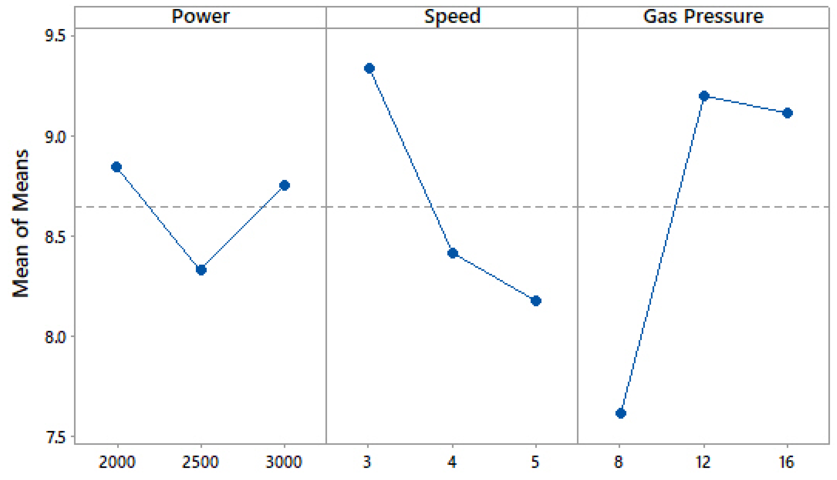
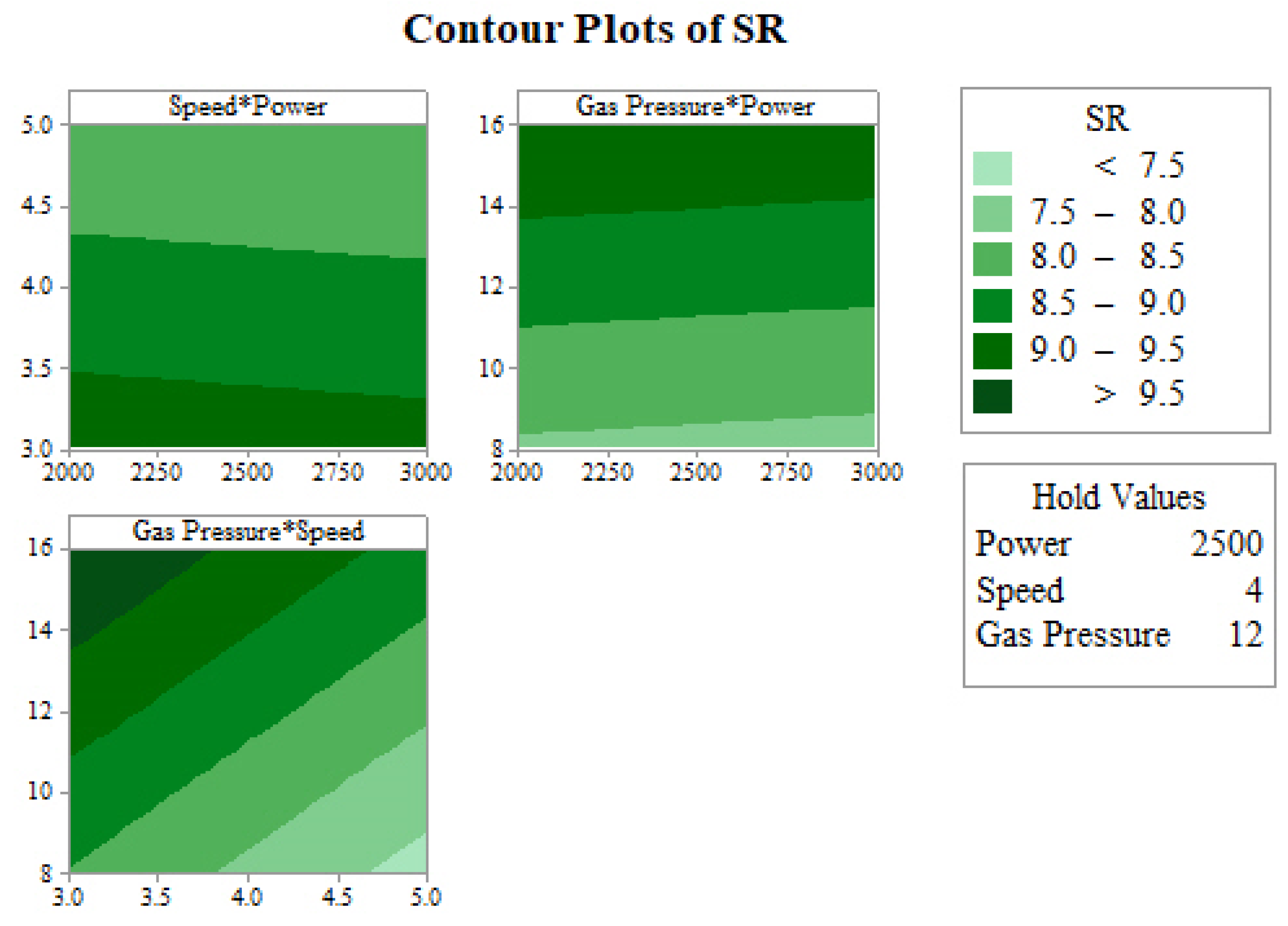
3.2. Analysis of Surface Roughness

In order to achieve optimal quality, the lowest possible value of SR is desirable. The ANOVA technique was used to investigate the significance of the selected input variable.

Table 4. ANOVA for SR.

Source	DF	SS	MS	F	p
Power	2	0.44823	0.22412	21.26	0.045
Speed	2	2.27344	1.13672	107.84	0.009
Gas pressure	2	4.76015	2.38007	225.80	0.004
Error	2	0.02108	0.01054
Total	8	7.50290

S = 0.1266, R-Sq. = 99.72%, R-Sq. (Adj.) = 98.88%.

shows the ANOVA table for SR. The significance of the input variables was determined on the basis of the F-value or the p-value. ANOVA analysis was conducted at a 95% confidence level. At a 95% confidence level, the p-value should be less than 0.05 to indicate that it has a significant effect on the selected response [38]. Table 4 shows that all of the machining parameters have a significant impact on SR, as the p-values for laser power, speed, and gas pressure were found to be 0.045, 0.009, and 0.004, respectively. The difference of less than 20% between the values of R-sq. and Adjusted (Adj.) R-sq. indicates that the existing model is suitable [39,40]. The R-sq. and Adj. R-sq. values for SR suggest that the model is able to provide the best fit for the existing data. The ANOVA results show that the contribution of gas pressure was the highest, at 63.44%, followed by cutting speed, with 30.3% contribution, and laser power, with 5.97% contribution. A negligible error contribution of 0.29% was observed, indicating that the present study could be effectively used as a basis for future predictions. Figure 2 shows a pie chart of the percentage contribution of machining variables for SR. The standard deviation for SR was observed to be 0.1226. This indicates that the maximum deviation from the mean value of SR is only 0.1226.

The impact of machining variables on SR on the basis of the main effect plot is shown in Figure 3. Main effect plots indicate the mean response of each level of the factors connected by the line. The Y-axis of the plot represents the mean of the means, i.e., the range of SR values obtained for different levels of the input machining parameters. It can be observed that increasing power results in a decrease in SR values, while a further increase in power results in increasing SR values. This is due to the heating supply in the machining zone. With a lower level of heat supply, the melted material has a higher viscosity and is not easily excluded from the machining zone [41]. However, at higher levels of heat supply, the higher temperature gradient may result in more molten material [26] and, as a result, the removal of the molten material from the cutting zone, thereby affecting the surface quality. Increasing cutting speed resulted in lower values of SR, which can mainly be attributed to the shorter exposure periods of the laser beam on the specimen [10,42]. An increase in SR was observed with increasing values of gas pressure. Increasing gas pressure generated more peaks and valleys in the cutting region, which in turn led to increased values of SR [42].

Figure 4 shows the residual plots for SR. Residual plots are important for verifying the ANOVA results [43]. The given four-in-one residual plots include a normal probability plot, a residual vs. fitted value plot, a histogram, and a residual vs. observation order plot. In the normality test, a straight line is formed by all of the residuals, as shown in Figure 4. It can be concluded that there is no residual clustering, and that these are all distributed normally. In the residual versus fitted plot, the allocation of all the residuals is random, which is a good method of statistical analysis for ANOVA. In the histogram plot, a parabolic structure can be observed, which supports the normality of the data. In the residual versus fitted plot, the absence of any pattern indicates the fitness of the ANOVA results. This verifies that all four tests confirm the satisfactory nature of future outcomes of the proposed model.

The influences of two simultaneous input variables (determined by keeping the third input variable constant) on SR were determined on the basis of the contour plots. Figure 5 shows the contour plots for SR. In the contour plot for speed and power, the horizontal axis represents power, and the vertical axis represents speed. This contour plot was generated by maintaining the value of gas pressure constant at the middle level (12 bar). The range of SR, which varied from 7.5 to 9.5 μm, is depicted using different colors in Figure 5. The lowest value of SR (<7.5 μm) was obtained by keeping the cutting speed in the range of 4.5 to 5 m/min, and with any value of laser power (between 2000 to 3000 W). The reason for this is that the higher cutting speed results in insufficient exposure of the specimen to the laser beam. The contour plot of gas pressure and power was generated by holding the cutting speed value at the middle level (4 m/min). The minimum value of SR (<7.5 μm) can be obtained when the gas pressure is around 8 bar, and for any value of laser power (between 2000 to 3000 W). In the contour plot of gas pressure and speed, the laser power was kept at a constant value of 2500 W. The lowest SR can be achieved at the lowest value of gas pressure and the maximum value of cutting speed used in the current study.

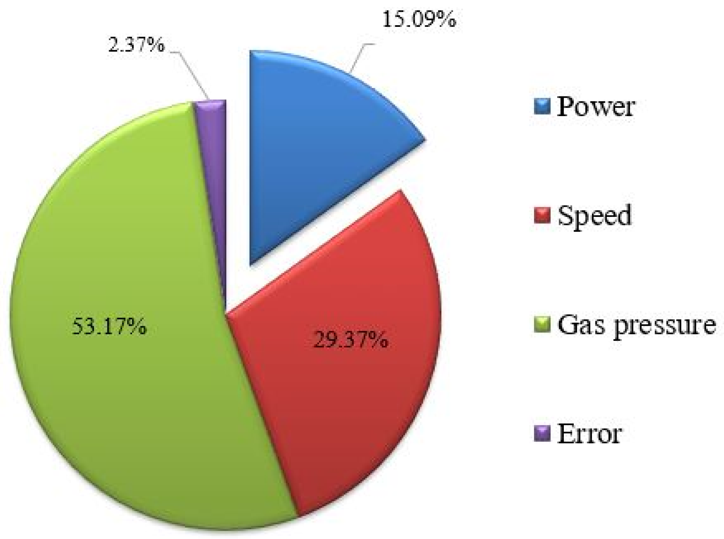
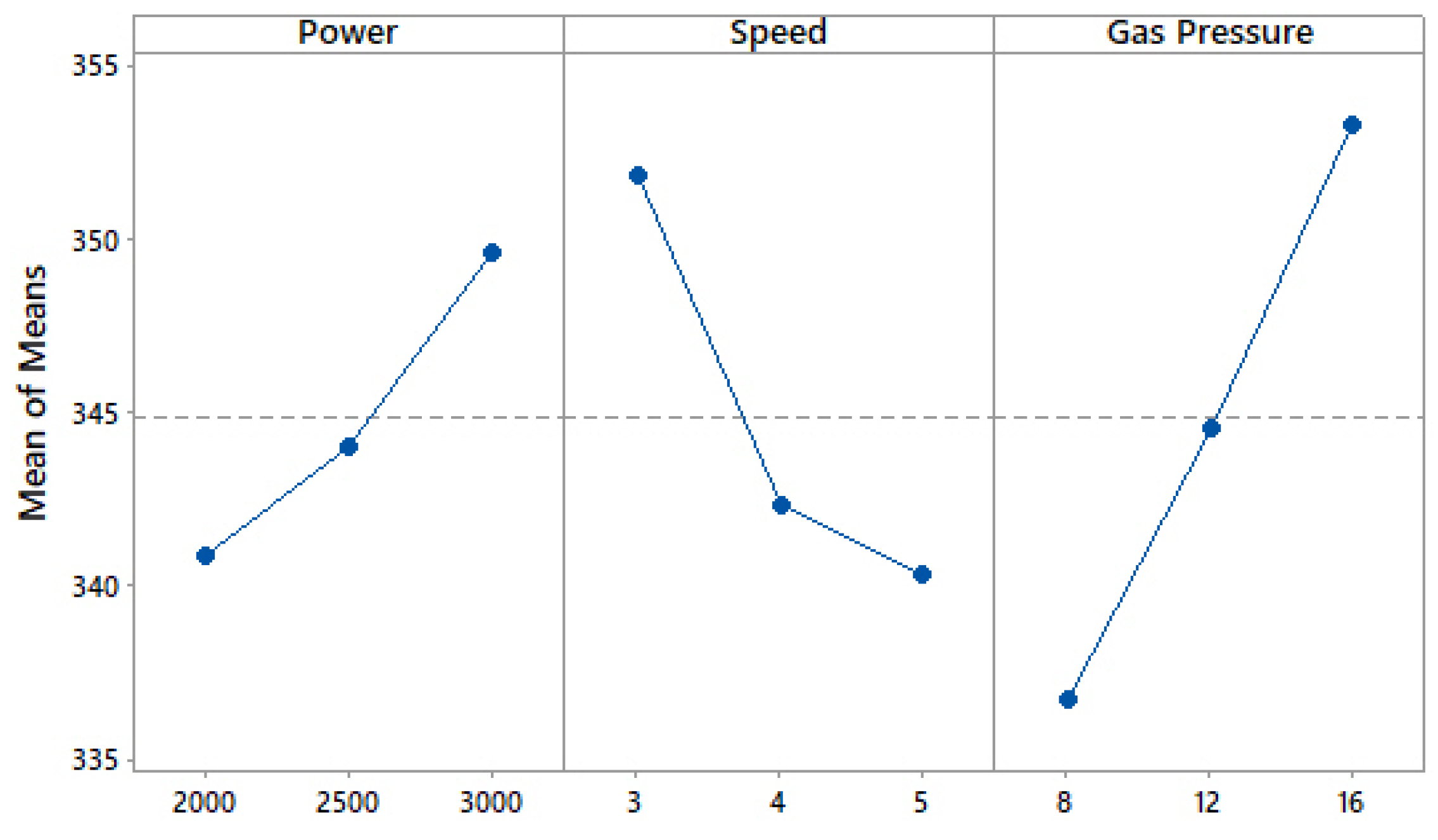
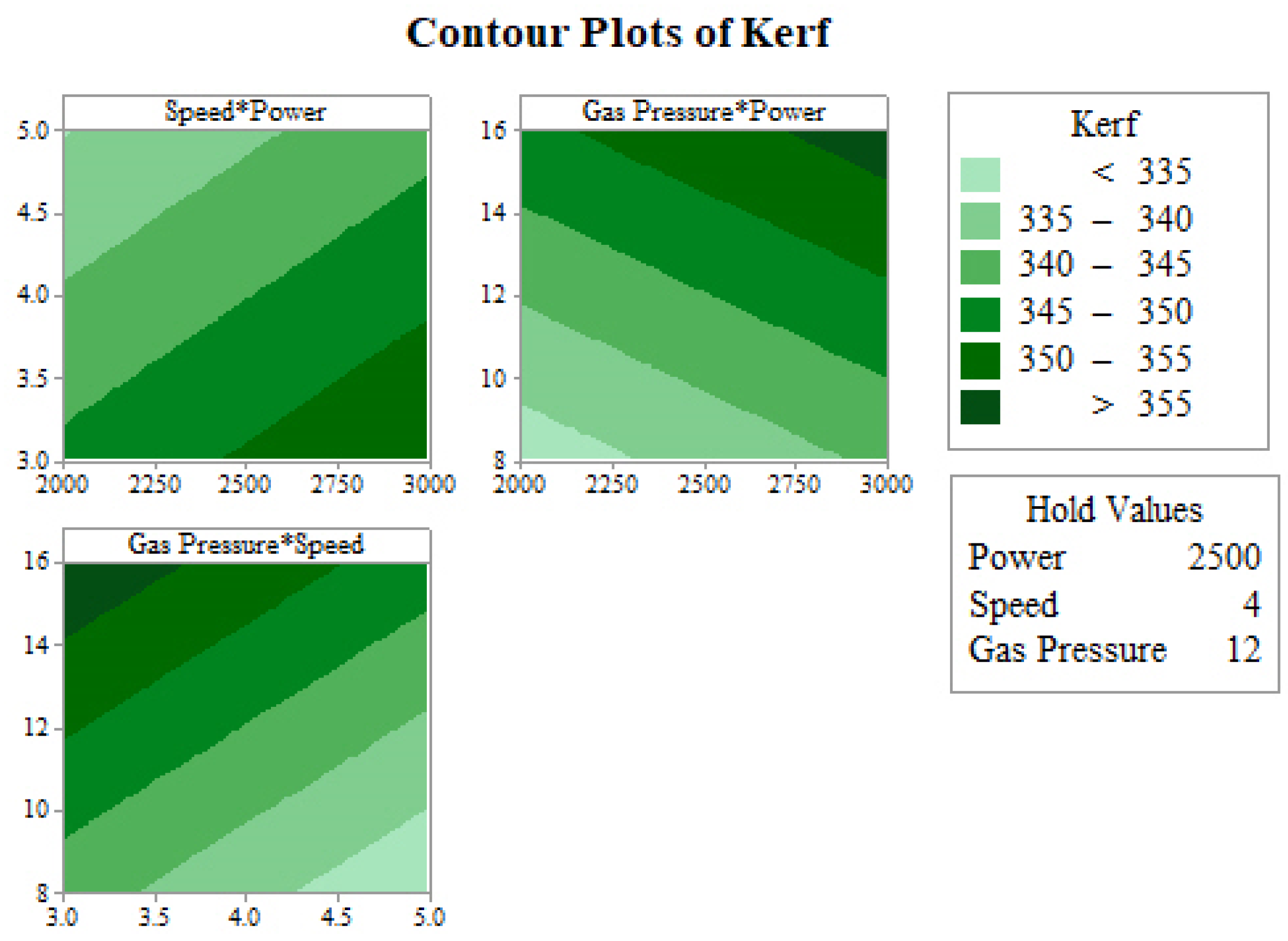
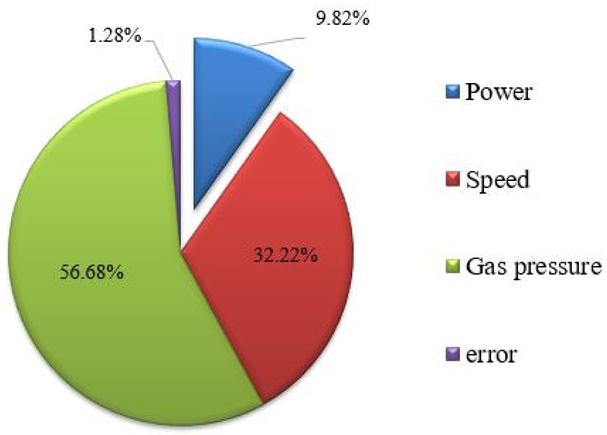
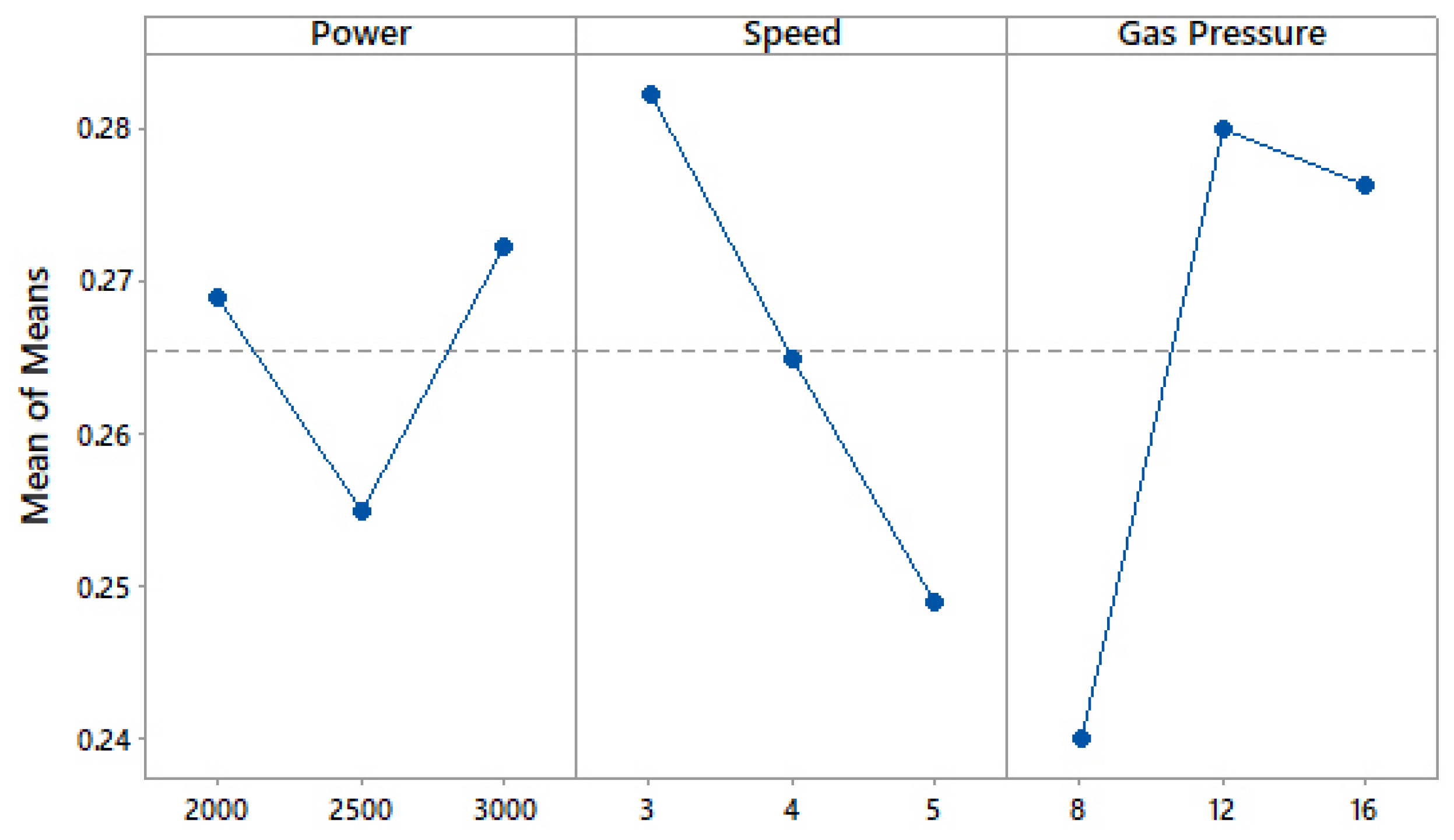
3.3. Analysis of Kerf Width

Table 5. ANOVA for kerf width.

Source	DF	SS	MS	F	p
Power	2	116.69	58.345	6.33	0.136
Speed	2	227.28	113.641	12.33	0.0175
Gas pressure	2	411.49	205.744	22.32	0.043
Error	2	18.44	9.218
Total	8	773.90

S = 3.036, R-Sq. = 97.62%, R-Sq. (Adj.) = 90.47%.

shows the ANOVA results for kerf width. ANOVA analysis was conducted at a 95% confidence level to identify the most significant effects of the input variables on the kerf width. Table 5 shows that the cutting speed and gas pressure have a significant impact on the kerf width, as the p-values for the speed and gas pressure can be observed to be less than 0.05. The difference between the values of R-sq. and Adj. R-sq. was less than 20%, which shows that the existing model is suitable for predicting future outcomes with minimal deviations. The ANOVA results show that the gas pressure has a significant impact on kerf width, with a 53.17% contribution, followed by cutting speed, with a 29.37% contribution, and laser power, with a 15.09% contribution. Figure 6 shows a pie chart of the percentage contribution of machining variables on kerf width. The standard deviation for SR was observed to be 3.036. This indicates that the maximum deviation from the mean value of SR is only 3.036.

Figure 7 shows the main effect plot for kerf width. The main effect plot of power vs. kerf shows an increase in the value of kerf width with increasing power. With higher heat supply to the machining zone, radial transfer of heat takes place in the material. Because of this higher energy, more material is vaporized from the cut edge, resulting in a wider kerf width [23]. A continuous decrement in kerf width was observed with increasing cutting speed. This was due to fact that the energy input at the cutting zone decreases with higher travel speed of the laser source [44]. An increase in the value of kerf width can be seen in Figure 7 with increasing gas pressure. Higher gas pressure creates greater force on the molten material, which increases the material removal rate [24].

Figure 8 shows the residual plots for kerf width. All four tests of the residual plot show good agreement, satisfying ANOVA results. This also shows the fitness of the proposed model for kerf with respect to improving future outcomes.

Figure 9 shows the contour plot of kerf width. The effects of two simultaneous machining variables on kerf width were studied by maintaining the third input variable at a constant value. In the contour plot of speed and power, a constant gas pressure value of 12 bar was used. The range of kerf width obtained for the given levels of the machining variables ranged from 335 to 350 μm. The minimum value of kerf (<335 μm) was obtained with a higher cutting speed (between 4.2 to 5 m/min) along with a lower laser power value (in the range of 2000 to 2250 W). For the contour plot of gas pressure and laser power, the lowest kerf width was obtained with a minimum gas pressure of 8 bar, while maintaining a minimum laser power in the range of 2000 to 2250 W. For the simultaneous effect of gas pressure and speed with a constant laser power of 2500 W, the minimum kerf width was achieved by maintaining a higher cutting speed, between 4.5 to 5 m/min, along with a lower value of gas pressure, 8 bar.

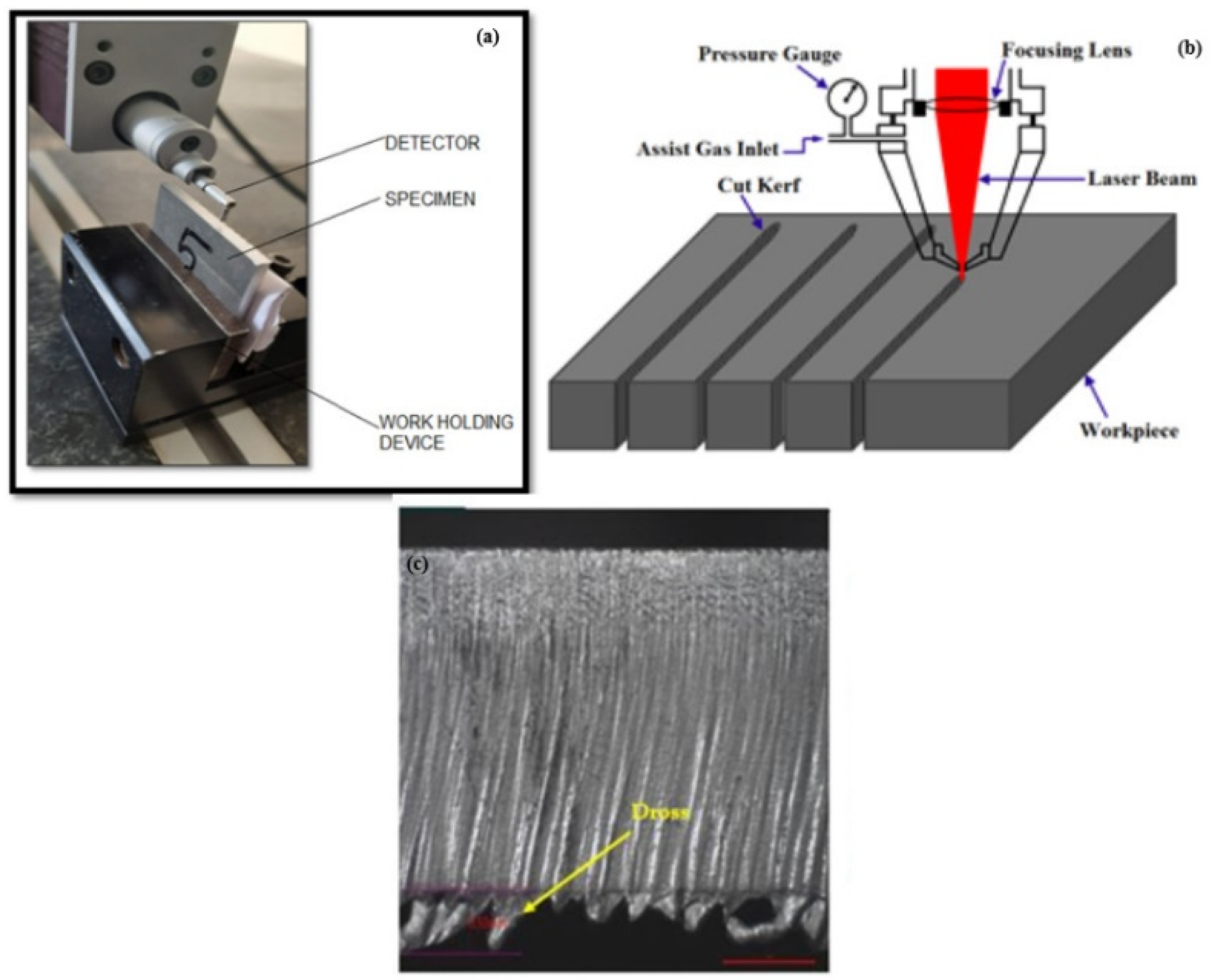
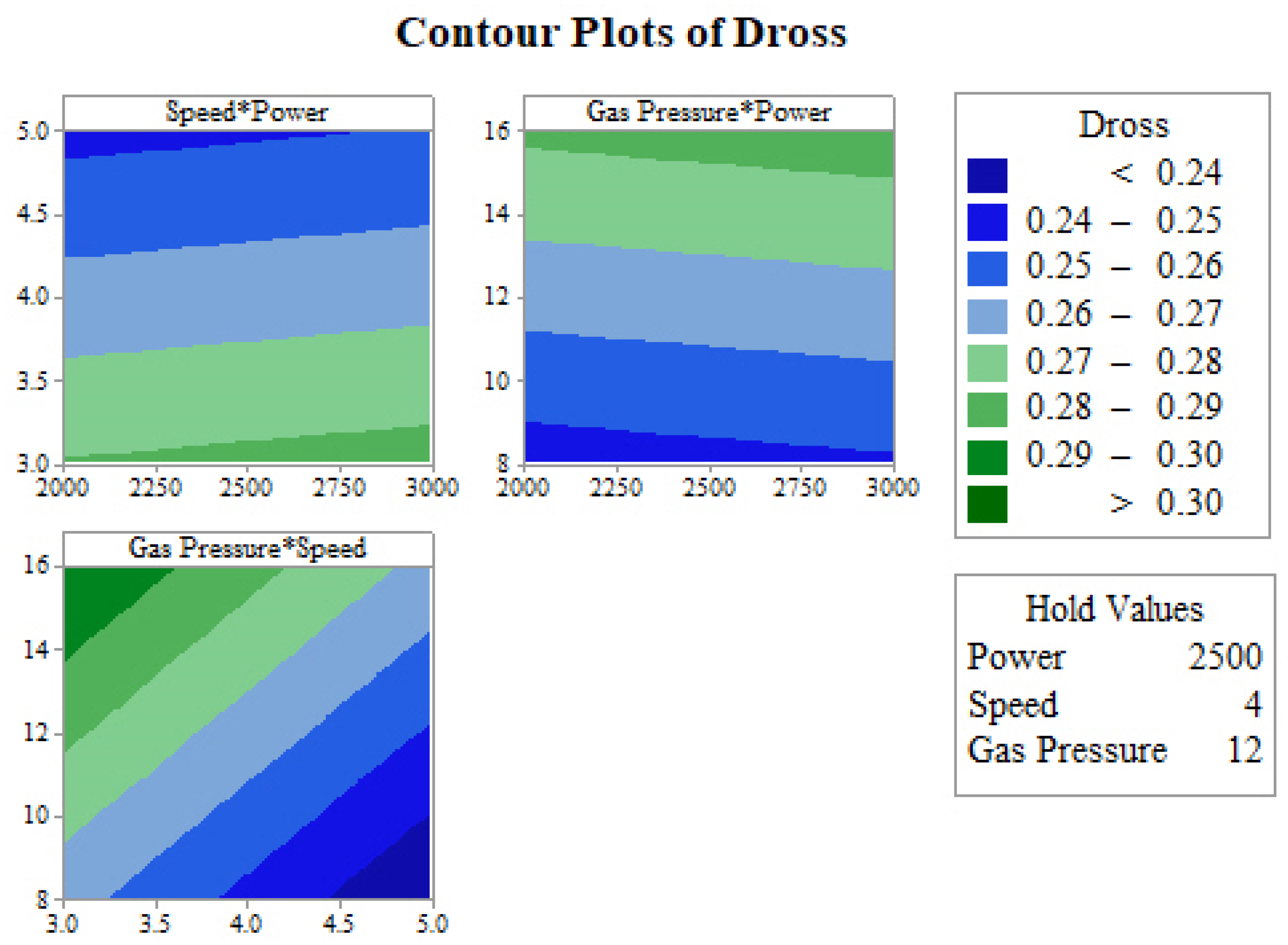
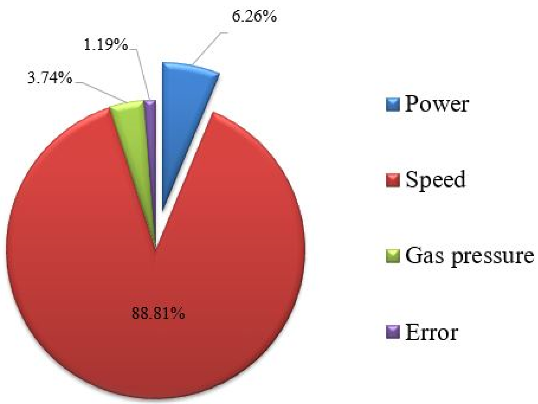
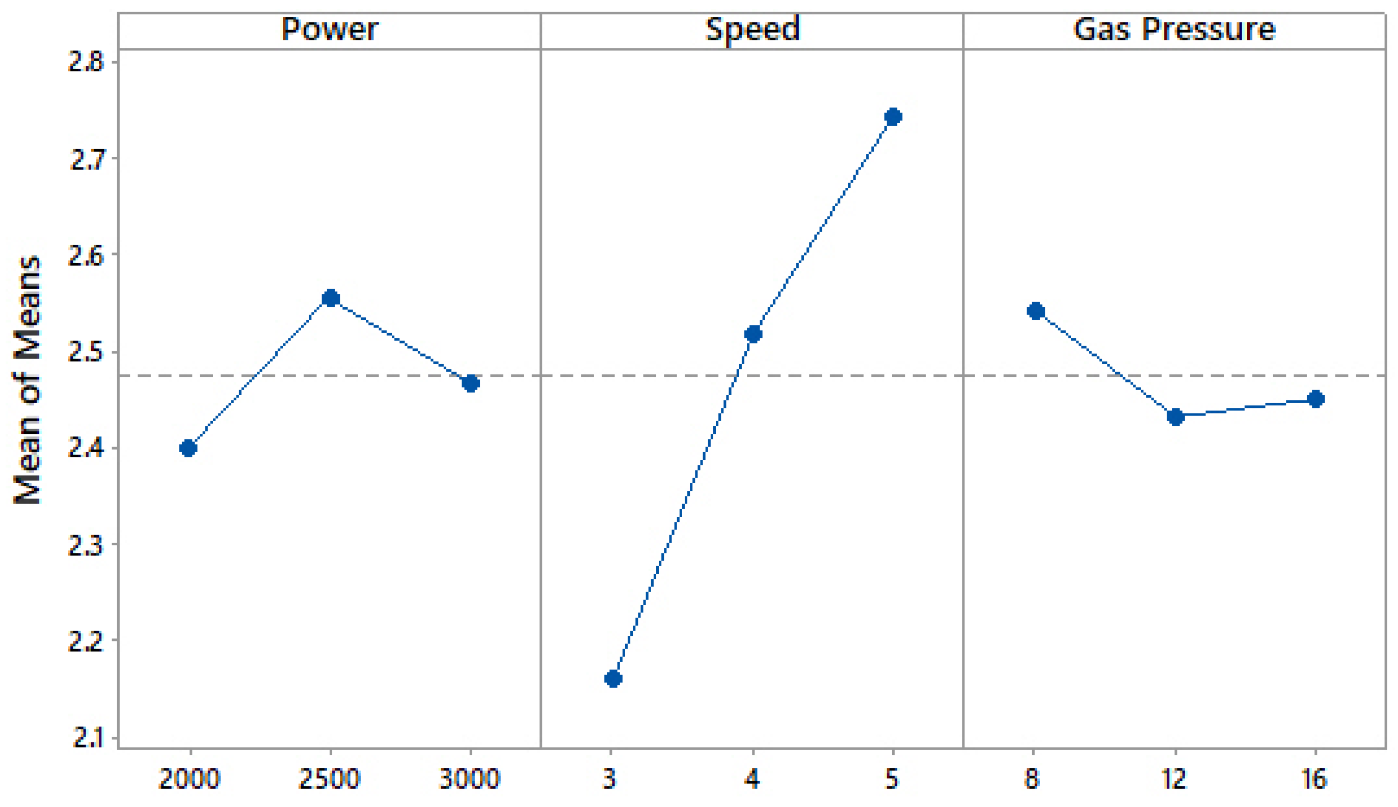
3.4. Analysis of Dross

The ANOVA technique was used for dross, as shown in

Table 6. ANOVA for Dross.

Source	DF	SS	MS	F	p
Power	2	0.000508	0.000254	7.51	0.117
Speed	2	0.001668	0.000834	24.68	0.039
Gas pressure	2	0.002934	0.001467	43.42	0.023
Error	2	0.000068	0.000034
Total	8	0.005176

S = 0.005811, R-Sq. = 98.69%, R-Sq. (Adj.) = 94.78%.

, to investigate the significance of the input variables with respect to the developed model. The ANOVA results for dross height indicate that the cutting speed and gas pressure have a significant impact on dross, as the p-values for the cutting speed and gas pressure were 0.039 and 0.023, respectively, which are both below the α value of 0.05. The R-sq. and R-sq. (adj.) values suggest that the model fits the existing data. The difference between both values is less than 20%. The ANOVA results show that gas pressure (56.68%) has the greatest effect on dross, followed by cutting speed (32.22%) and laser power (9.82%). A negligible error contribution of 1.29% was observed, which indicates that the present study can be effectively used as a basis for future predictions. Figure 10 presents a pie chart of the percentage contributions of machining variables with respect to dross. The standard deviation for dross was observed to be 0.005811, indicating that the maximum deviation from the mean value of dross is much lower.

The impact of machining variables on dross is depicted in Figure 11. It can be observed that with increasing laser power, dross height decreases. Further increases in laser power showed the reverse effect, increasing the value of dross height. It can be observed that increasing cutting speed results in decreased dross height. This is due to the heat energy supplied at the cut edge, and is dependent on the laser power and cutting speed [9]. The temperature of the cut edge changes the force magnitude (i.e., the assist gas force for removing the molten material) and direction. At lower values of cut edge temperature, the magnitude of the gas force is lower, and the direction is also away from the centerline. Meanwhile, in cases with higher cut edge temperatures, the magnitude of the gas force is higher, but the direction is far away from the centerline. Therefore, the optimal selection of power and speed will effectively exclude molten material while resulting in minimal dross [9]. An increase in dross was observed with increasing gas pressure. Vibration and unstable conditions were observed at higher gas pressure, resulting in poor machining quality. Additionally, the cooling effect was comparatively greater at higher gas pressure, which in turn helps in the re-solidification of molten material and results in more dross [45].

Figure 12 shows the residual plots for dross. All four tests of the residual plot for dross show good agreement similar to SR and kerf width which satisfies the ANOVA results. This also shows a good fit of the proposed model for dross.

The influences of two simultaneous input variables (by keeping the third input variable constant) on dross height were determined with the help of contour plots. Figure 13 shows the contour plot for dross height. The contour plot of speed and power was generated by holding the gas pressure value constant at 12 bar. The range of dross height was varied from 0.24 to 0.30 mm. The lowest value of dross (<0.24 mm) was obtained with a maximum cutting speed of 5 m/min along with a laser power in the range of 2000 to 2500 W. The contour plot of gas pressure and power was generated by holding the cutting speed value at the middle level (4 m/min). A minimum value of dross height (<0.24 mm) was obtained with a minimum gas pressure of around 8 bar and any value of laser power (between 2000 and 3000 W). In the contour plot of gas pressure and speed, the laser power was kept at a constant value of 2500 W. The lowest dross height was obtained at the maximum value of cutting speed and the lowest value of gas pressure.

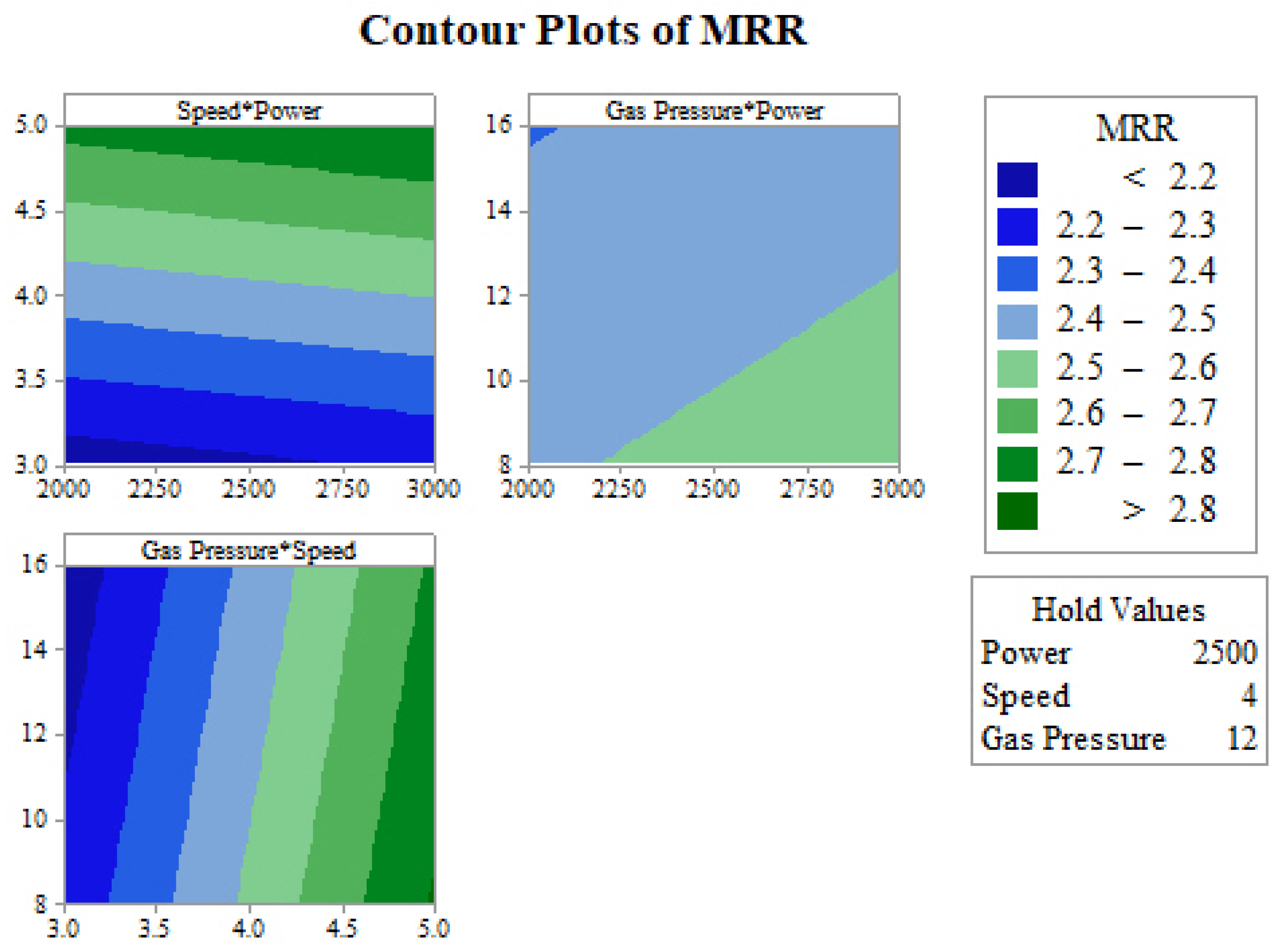
3.5. Analysis of Material Removal Rate

A higher value of MRR is always desirable, as it increases productivity, which in turn results in savings with respect to cost, time, and other expenses.

Table 7. ANOVA for MRR.

Source	DF	SS	MS	F	p
Power	2	0.036234	0.018117	5.27	0.159
Speed	2	0.514433	0.257216	74.84	0.013
Gas pressure	2	0.021687	0.010843	3.16	0.241
Error	2	0.006874	0.003437
Total	8	0.579227

S = 0.05862, R-Sq. = 98.81%, R-Sq. (Adj.) = 95.25%.

shows the ANOVA results for MRR. ANOVA analysis was conducted at a 95% confidence level to identify the most significant effects of input variables on MRR. Table 6 shows that cutting speed has a significant effect on MRR, as the p-value for gas pressure was observed to be 0.013, which is less than 0.05. The difference of less than 20% between the values of R-sq. and R-sq. (Adj.) indicates that the present model is suitable for predicting future outcomes with few deviations. The ANOVA result shows that the significance of cutting speed was the highest, with a contribution of 88.81%, followed by laser power, with a contribution of 6.26%, and gas pressure, with a contribution of 3.74%. An error contribution of 1.19% was observed, which shows that the present study can be used as the basis for future predictions. Figure 14 presents a pie chart of the percentage contributions of machining variables towards MRR. The standard deviation for MRR was observed to be 0.05862. This shows that the maximum deviation from the mean value of MRR was only 0.05862.

Figure 15 shows the main effect plot for MRR. The initial increase in laser power resulted in an increase in MRR, while a further increment in power resulted in lower MRR. Heat supply to the machining zone increases with increasing power, which in turn results in material melting in a shorter time, which in turn increases MRR [45]. At the highest laser power, more material is melted in the machining zone. This melted material is removed from the work specimen, resulting in lower values of MRR at higher values of laser power [45]. A continuous increase in MRR was observed with increasing cutting speed. MRR is largely dependent on cutting speed. The main effect plot for gas pressure showed no significant effect on MRR.

Figure 16 shows the residual plots of MRR. All four tests of the residual plot show good agreement, satisfying the ANOVA results. This also shows the fitness of the proposed model for optimizing kerf in order to obtain better future outcomes.

Figure 17 shows the contour plot of MRR. The effects of two simultaneous machining variables were studied by holding the third input variable constant with respect to MRR. In the contour plot of speed and power, a constant gas pressure value of 12 bar was used. The range of MRR obtained for the given levels of the machining variables ranged from 2.2 to 2.8 g/s. The maximum MRR (>2.8 g/s) was attained at a higher cutting speed along with any value of laser power in the range of 2000 to 3000 W. Regarding the contour plot of gas pressure and power, a maximum MRR of about 2.6 g/s was obtained at higher power and lower gas pressure. Regarding the simultaneous effect of gas pressure and speed with a constant laser power of 2500 W, a maximum MRR (>2.8 g/s) could be achieved when maintaining a higher cutting speed of between 4.5 and 5 m/min along with any value of gas pressure between 8 and 16 bar.

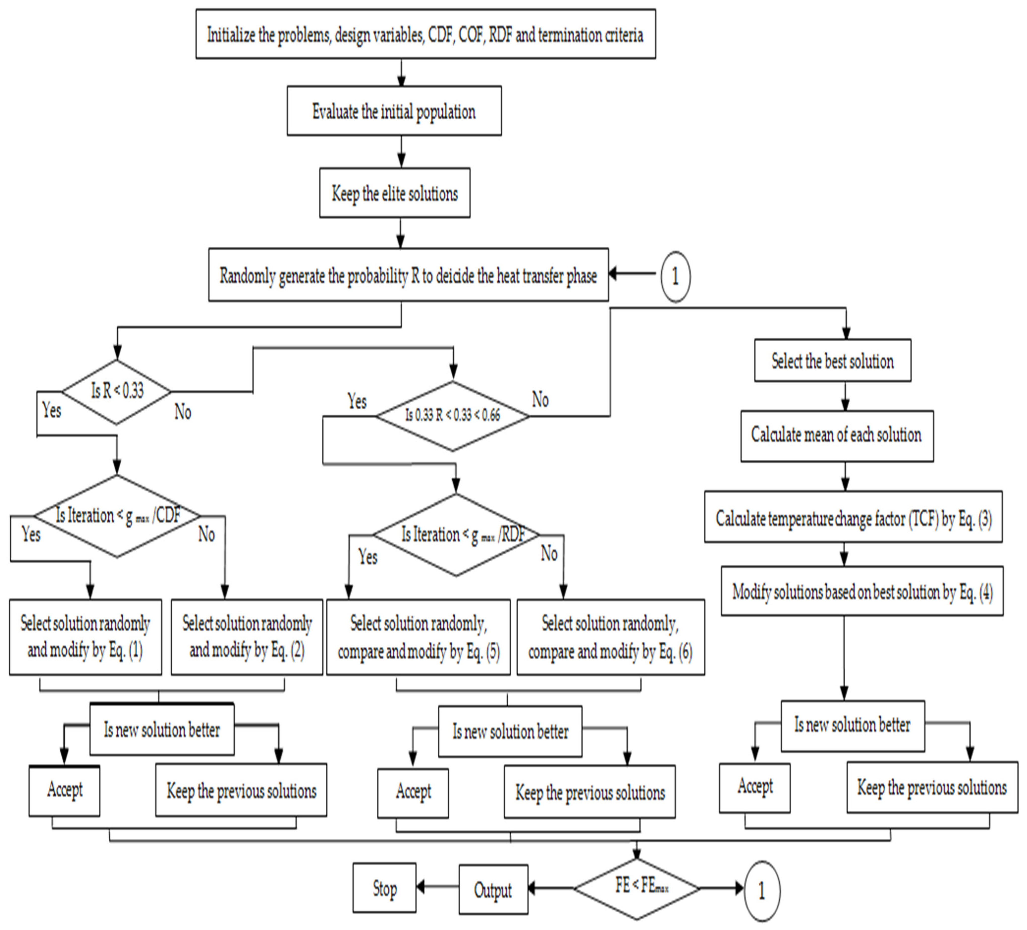
3.6. Optimization Using Heat Transfer Search Algorithm

The HTS algorithm, proposed by Patel and Savsani [18], works on heat transfer due to the interaction between the system molecules and with the surroundings to reach thermal equilibrium. Thermal equilibrium can be achieved as a result of three heat transfer phenomena: conduction, convection, and radiation. To obtain an equilibrium state, the HTS algorithm makes use of the three phases of heat transfer. The conduction, convection and radiation phases have equal opportunity to achieve heat transfer. For each generation, one of the modes of heat transfer is selected randomly. The HTS algorithm starts by selecting a randomly generated population. In a randomly generated population, the system has a number of molecules ‘n’ and a temperature level. The population is then updated in each generation using one of the randomly selected heat transfer modes. Moreover, the updated solution in the HTS algorithm is accepted if it has a better functional value. Subsequently, the worst solutions of the population are replaced by better solutions [40]. Figure 18 shows the flowchart of the HTS algorithm.

3.6.1. Conduction Phase

The solutions were updated in the conduction phase as per Equations (6) and (7), below:

$$X_{j,i}^{\prime }=\{\begin{array}{c}{X}_{k,i}+\left(-R^2{X}_{k,i}\right), iff\left(X_j\right)>f\left(X_k\right)\\ X_{j,i}+\left(-R^2{X}_{j,i}\right), iff\left(X_j\right)<f\left(X_k\right)\end{array};ifg\le \raisebox{1ex}{$g_{\max }$}\!\left/ \!\raisebox{-1ex}{$CDF$}\right.$$

(6)

$$X_{j,i}^{\prime }=\{\begin{array}{c}{X}_{k,i}+\left(-r_i{X}_{k,i}\right), iff\left(X_j\right)>f\left(X_k\right)\\ X_{j,i}+\left(-r_i{X}_{j,i}\right), iff\left(X_j\right)<f\left(X_k\right)\end{array};ifg>\raisebox{1ex}{$g_{\max }$}\!\left/ \!\raisebox{-1ex}{$CDF$}\right.$$

(7)

where $X_{j,i}^{\prime }$ is the updated solution; j = 1,2,…, n; k is a randomly selected solution; j ≠ k; k $\in$ (1,2,…, n); i is a randomly selected design variable; i $\in$ (1,2,…, m); g_max is the maximum number of generation specified; CDF is the conduction factor; R is the probability variable; R $\in${0, 0.3333}; and r_i$\in${0, 1} is a uniformly distributed random number.

3.6.2. Convection Phase

The solutions were updated in the convection phase as per Equations (8) and (9), below:

$$X_{j,i}^{\prime }=X_{j,i}+R\times \left(X_s-X_{ms}\times TCF\right)$$

(8)

$$TCF=\{\begin{array}{c}abs\left(R-r_i\right), ifg\le \raisebox{1ex}{$g_{\max }$}\!\left/ \!\raisebox{-1ex}{$COF$}\right.\\ round\left(1+r_i\right), ifg>\raisebox{1ex}{$g_{\max }$}\!\left/ \!\raisebox{-1ex}{$COF$}\right.\end{array}$$

(9)

where $X_{j,i}^{\prime }$ is the updated solution; j = 1,2,…, n; i = 1,2,…, m. COF is the convection factor; R is the probability variable; R $\in${0.6666, 1}; r_i$\in${0, 1} is a uniformly distributed random number; X_s is the temperature of the surroundings; X_ms is the mean temperature of the system; and TCF is the temperature change factor.

3.6.3. Radiation Phase

The solutions were updated in the radiation phase as per Equations (10) and (11), below:

$$X_{j,i}^{\prime }=\{\begin{array}{c}{X}_{j,i}+R\times \left(X_{k,i}-X_{j,i}\right), iff\left(X_j\right)>f\left(X_k\right)\\ X_{j,i}+R\times \left(X_{j,i}-X_{k,i}\right), iff\left(X_j\right)<f\left(X_k\right)\end{array};ifg\le \raisebox{1ex}{$g_{\max }$}\!\left/ \!\raisebox{-1ex}{$RDF$}\right.$$

(10)

$$X_{j,i}^{\prime }=\{\begin{array}{c}{X}_{j,i}+r_i\times \left(X_{k,i}-X_{j,i}\right), iff\left(X_j\right)>f\left(X_k\right)\\ X_{j,i}+r_i\times \left(X_{j,i}-X_{k,i}\right), iff\left(X_j\right)<f\left(X_k\right)\end{array};ifg>\raisebox{1ex}{$g_{\max }$}\!\left/ \!\raisebox{-1ex}{$RDF$}\right.$$

(11)

where $X_{j,i}^{\prime }$ is the updated solution; j = 1, 2,…, n; i = 1, 2, …, m; j ≠ k; k $\in$ (1, 2, …, n) and k is a randomly selected molecule; RDF is the radiation factor; R is the probability variable; R $\in${0.3333, 0.6666}; r_i$\in${0, 1} is a uniformly distributed random number.

During the implementation of the HTS algorithm, all of the objectives (SR, dross, kerf, MRR) were considered to be positive integers. The extreme machining limits of the used set-up were considered during the implementation of the algorithms.

• Power: 1000 W ≤ Power ≥ 3000 W
• Cutting speed: 1 m/min ≤ Speed ≥ 8 m/min
• Gas pressure: 6 bar ≤ Gas pressure ≥ 20 bar

By considering the extreme machining limits, single-objective optimization was carried out for SR, kerf, dross, and MRR, as seen in

Table 8. Results of single-objective optimization.

Objective Function	Design Variables			Objective Function
	Power (W)	Speed (m/min)	Gas Pressure (Bar)	SR (µm)	Kerf (µm)	Dross (mm)	MRR (g/s)
Minimum SR	3000	8	6	5.13	313.78	0.1721	3.738
Minimum Kerf	1000	8	6	5.32	296.38	0.1661	3.606
Minimum Dross	1000	8	6	5.32	296.38	0.1661	3.606
Maximum MRR	3000	8	6	5.13	313.78	0.1721	3.738

. Minimum surface roughness is always desirable for any machined part in order to best fulfill its function during application. The narrowness of the kerf width is a major advantage of the laser process, as it reduces the amount of scrap metal and enhances the cut quality. Minimum kerf width is essential for any cutting, slitting, or trimming process. The minimum value of dross is desirable for achieving better machining quality. A higher value of MRR is always desirable, as it increases productivity, which in turn saves cost, time, and other expenses. On this basis, single-objective optimization was carried out for minimum SR, minimum kerf, minimum dross, and maximum MRR.

Simultaneous optimization was also carried out for all of the selected output responses—SR, kerf, dross, and MRR—by giving an equal weight of 0.25 to all output responses. Equation (12) presents the objective function for simultaneous optimization.

$$Obj=w_1·\left(SR\right)+w_2·\left(\mathrm{kerf}\right)+w_3·\left(\mathrm{dross}\right)+w_4·\left(MRR\right)$$

(12)

The corresponding machining variables of a laser power of 1742 W, a cutting speed of 8 m/min, and a gas pressure of 6 bar were observed to provide the optimum values for the present objective function. The results obtained with these parameters were an SR value of 5.25 µm, a kerf of 302.83 µm, a dross of 0.1684 mm, and an MRR of 3.65. However, different users have different requirements. To tackle such situations, multi-objective optimization along with non-dominated optimal solutions were generated. For multi-objective optimization, the MOHTS technique was implemented. MOHTS is an acronym for “multi-objective heat transfer search”, and is the multi-objective version of the HTS algorithm. It is able to handle two-or-more-output responses, and creates non-dominant solutions for input variables [46]. The MOHTS algorithm was used to generate 49 non-dominant Pareto optimal points for all of the output responses, as shown in

Table 9. Predicted results of the HTS algorithm.

Sr. No.	Power (W)	Speed (m/min)	Gas Pressure (Bar)	SR (µm)	Kerf (µm)	Dross (mm)	MRR (g/s)
1	1000	8	6	5.32	296.38	0.1661	3.606
2	3000	8	6	5.13	313.78	0.1721	3.738
4	2404	8	6	5.19	308.59	0.1703	3.698
5	1119	8	6	5.31	297.41	0.1665	3.613
6	2642	8	6	5.16	310.66	0.1711	3.714
7	1742	8	6	5.25	302.83	0.1684	3.654
8	2886	8	6	5.14	312.79	0.1718	3.730
9	2177	8	6	5.21	306.62	0.1697	3.683
10	1904	8	6	5.23	304.24	0.1688	3.665
11	2475	8	6	5.18	309.21	0.1706	3.703
12	2584	8	6	5.17	310.16	0.1709	3.710
13	2037	8	6	5.22	305.40	0.1692	3.674
14	2695	8	6	5.16	311.13	0.1712	3.717
15	2560	8	6	5.17	309.95	0.1708	3.708
16	2757	8	6	5.15	311.66	0.1714	3.721
17	2114	8	6	5.21	306.07	0.1695	3.679
18	1183	8	6	5.30	297.97	0.1667	3.618
19	1243	8	6	5.30	298.49	0.1669	3.622
20	2944	8	6	5.13	313.29	0.1720	3.734
21	1802	8	6	5.24	303.36	0.1685	3.658
22	2235	8	6	5.20	307.12	0.1698	3.687
23	1959	8	6	5.23	304.72	0.1690	3.669
24	2151	8	6	5.21	306.39	0.1696	3.681
25	2930	8	6	5.14	313.17	0.1719	3.733
26	2845	8	6	5.14	312.43	0.1717	3.727
27	1342	8	6	5.29	299.35	0.1672	3.628
28	2509	8	6	5.18	309.51	0.1707	3.705
29	1017	8	6	5.32	296.53	0.1662	3.607
30	2372	8	6	5.19	308.32	0.1702	3.696
31	2681	8	6	5.16	311.00	0.1712	3.716
32	1200	8	6	5.30	298.12	0.1667	3.619
33	1085	8	6	5.31	297.12	0.1664	3.611
34	1995	8	6	5.23	305.04	0.1691	3.671
35	1545	8	6	5.27	301.12	0.1678	3.641
36	1295	8	6	5.29	298.95	0.1670	3.625
37	1390	8	6	5.28	299.77	0.1673	3.631
38	1705	8	6	5.25	302.51	0.1682	3.652
39	1054	8	6	5.32	296.85	0.1663	3.609
40	2795	8	6	5.15	312.00	0.1715	3.724
41	2072	8	6	5.22	305.71	0.1693	3.676
42	1467	8	6	5.28	300.44	0.1675	3.636
43	2079	8	6	5.22	305.77	0.1694	3.677
44	1840	8	6	5.24	303.69	0.1687	3.661
45	1638	8	6	5.26	301.93	0.1680	3.648
46	1502	8	6	5.27	300.75	0.1676	3.639
47	2283	8	6	5.20	307.54	0.1700	3.690
48	1577	8	6	5.27	301.40	0.1679	3.644
49	1876	8	6	5.24	304.00	0.1688	3.663

. All of these points give an optimum solution for SR, kerf, dross, and MRR for individual input variables. Table 9 shows 49 feasible optimal Pareto points. Each optimal solution shown in Table 9 is independent and unique. Therefore, depending on the requirements of the required output response values, users can select different levels of the corresponding input variables. Furthermore, whenever any decision variable creates a conflicting effect with respect to the objective function (i.e., output response), the discrete variation of that variable can be observed to be between the upper and lower limit. If the decision variable does not create a conflicting effect with respect to the output response, a constant value of that variable can be observed at all Pareto points. In the present work, the cutting speed and gas pressure create similar effects (i.e., there is no conflict effect) on the output response, and hence a constant value for both parameters (cutting speed of 8 m/min and gas pressure of 6 bar) can be observed at all Pareto points. Validation studies were conducted by randomly selecting five Pareto optimal points to verify the adequacy of the HTS algorithm.

Table 10. Confirmatory trials of Pareto optimal points.

Sr. No.	Power (W)	Speed (m/min)	Gas Press. (Bar)	Predicted Values by HTS Algorithm				Measured Values by HTS Algorithm				% Deviation
				SR	kerf	Dross	MRR	SR	kerf	Dross	MRR	SR	kerf	Dross	MRR
4	2404	8	6	5.19	308.59	0.1703	3.698	5.17	302.55	0.1723	3.654	0.38	1.99	1.16	1.2
10	1904	8	6	5.23	304.24	0.1688	3.665	5.26	308.38	0.1679	3.599	0.57	1.34	0.53	1.83
32	1200	8	6	5.30	298.12	0.1667	3.619	5.38	301.41	0.1675	3.544	1.5	1.09	0.47	2.11
40	2795	8	6	5.15	312.00	0.1715	3.724	5.18	307.34	0.1703	3.694	0.57	1.49	0.70	0.81
49	1876	8	6	5.24	304.00	0.1688	3.663	5.28	305.98	0.1679	3.701	0.75	0.65	0.53	1.02

presents the confirmatory trials conducted for the five Pareto optimal points, along with the experimentally measured values for all of the response variables. A negligible difference can be observed between the experimentally measured values and the values predicted by the HTS algorithm. This confirms that the existing HTS algorithm, along with the proposed model, is highly capable and suitable for fiber laser cutting of Ti6Al4V.

3D and 2D plots were prepared using non-dominant optimal Pareto points, as shown in Table 9. As the minimum values of SR, kerf, and dross are desirable for the laser machining of Ti6Al4V, a 3D plot for these three output response variables was generated, as shown in Figure 19. In the 3D Pareto plot, the X-axis represents the kerf values, the Y-axis represents the dross values, and the Z-axis represents the SR values. However, the values represented in the 3D plots include the effect of the remaining output response variables, i.e., MRR. Each point represented on the 3D Pareto curve gives a unique solution, with its own corresponding input process parameters. The operator can select any Pareto point on the curve, depending on the required values of output responses, to obtain the corresponding values of input process parameters that can be used for machining.

By considering the need for industrial users/operators, 2D plots were also generated. Figure 20a–c show three different 2D plots, corresponding to MRR vs. kerf, MRR vs. SR, and MRR vs. dross. However, the values presented in these 2D plots include the effect of the other two response variables. 2D Pareto curves are more useful when the other two response variables are not desirable for the users. Figure 20a represents the 2D Pareto curve of MRR vs. kerf, in which the X-axis represents the kerf values and the Y-axis represents the MRR values. The machining parameter corresponding to the red point mentioned on the curve indicates that the maximum MRR can be achieved under this machining condition. However, at the same time, the kerf value will be increased, which is not desirable. A similar situation can be observed for the machining parameters, represented by a yellow point, which can provide the desired minimum kerf value, while resulting in decreased values of MRR, which is not desirable. Therefore, the operator can select any optimal point of the curve on the basis of the required values of MRR and kerf. Figure 20b shows the 2D Pareto curve of MRR vs. SR, in which the X-axis represents the SR values and the Y-axis represents the MRR values. The green point on the curve describes the machining conditions under which the desired higher MRR and lower SR can be achieved simultaneously. Figure 20c shows the 2D Pareto curve of MRR vs. dross. The selection of the Pareto point for maximum MRR will result in a higher value of dross (represented by the red point). On the other hand, the Pareto point for lower dross will also result in a decreased value of MRR (represented by the yellow point). Therefore, again depending on the required values of MRR and dross, the optimal point on the curve can be selected, which provides the corresponding machining variables.

4. Conclusions

In the current study, the influence of different process parameters of the fiber laser cutting process was analyzed with respect to the output response variables of Ti6Al4V. Laser power, cutting speed, and gas pressure were selected as the input process parameters, while SR, kerf width, dross height, and MRR were considered as the output variables. The following conclusions can be drawn from the current study:

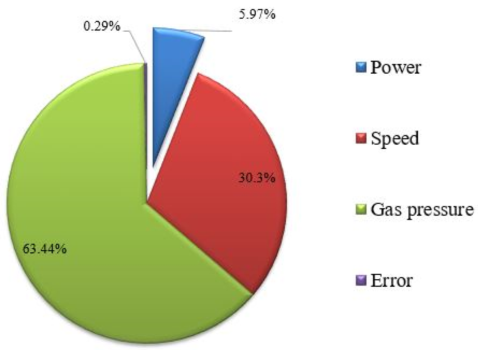
• The ANOVA results of SR show that all three machining variables were found to be significant, with the highest contribution of 63.44% being for gas pressure, followed by the cutting speed, with a 30.3% contribution, and laser power, with a 5.97% contribution. The ANOVA results of kerf demonstrated the significant effect of cutting speed (53.17%) and gas pressure (29.37%). For dross height, the cutting speed and gas pressure were observed to have a significant effect, while for MRR, the cutting speed had a significant effect.
• Regression equations were generated for each response variable that was found to be robust from ANOVA. This model is helpful for the prediction of output responses for the manufacturing of components in industry without conducting the actual experiments.
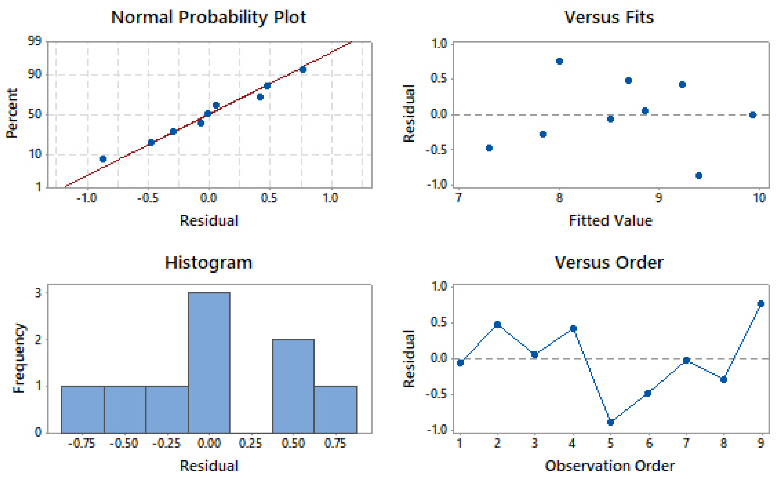
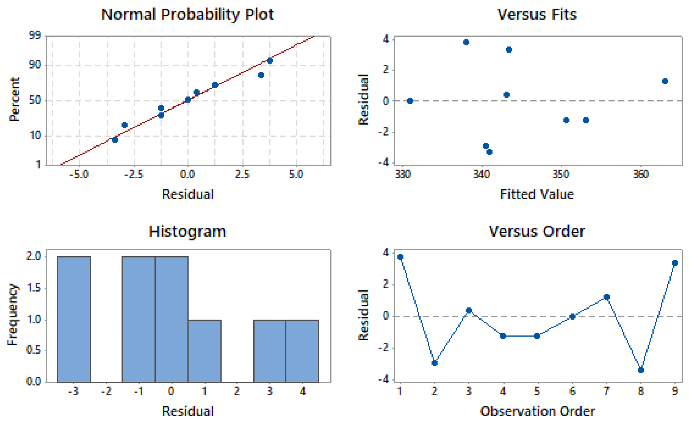
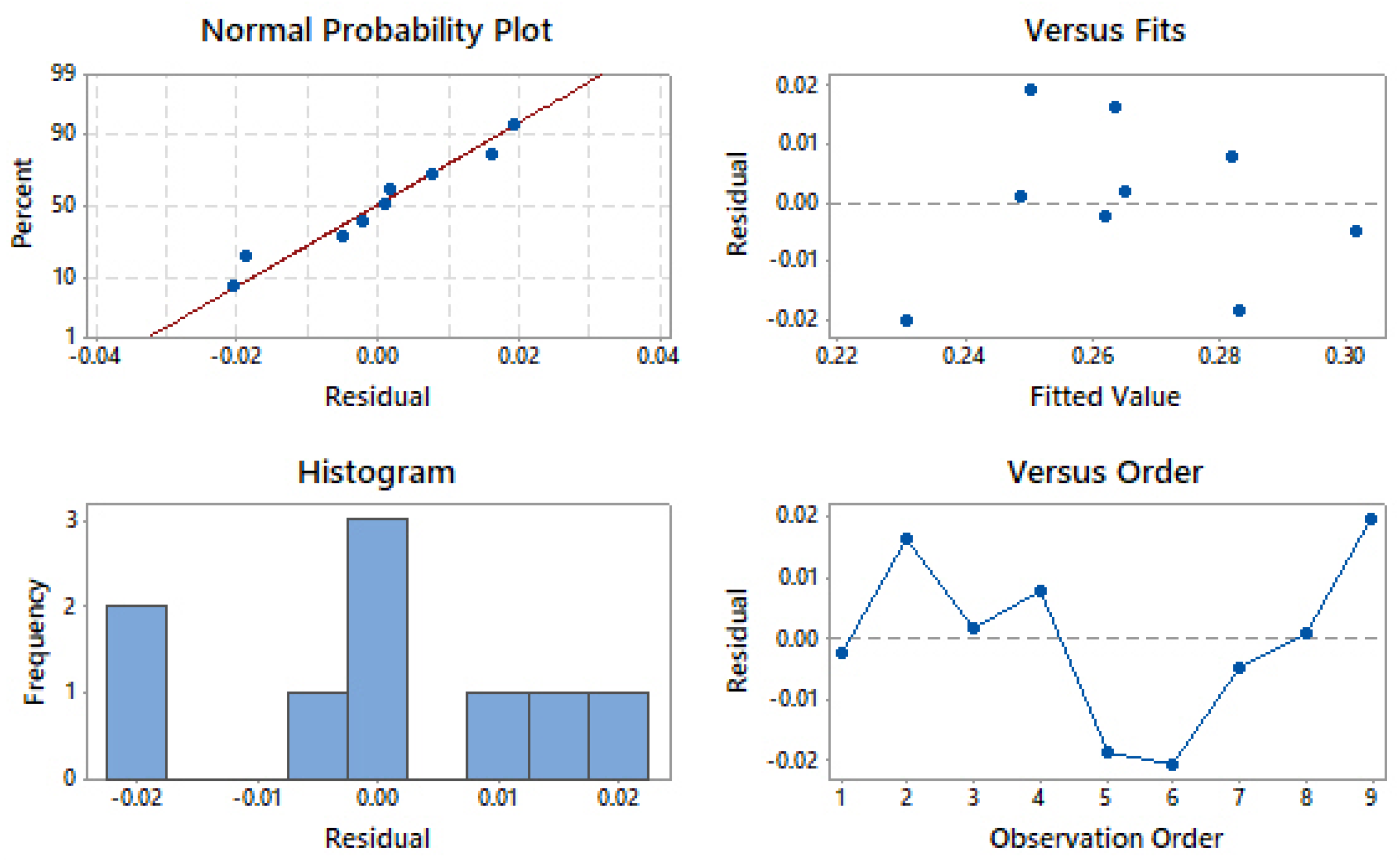
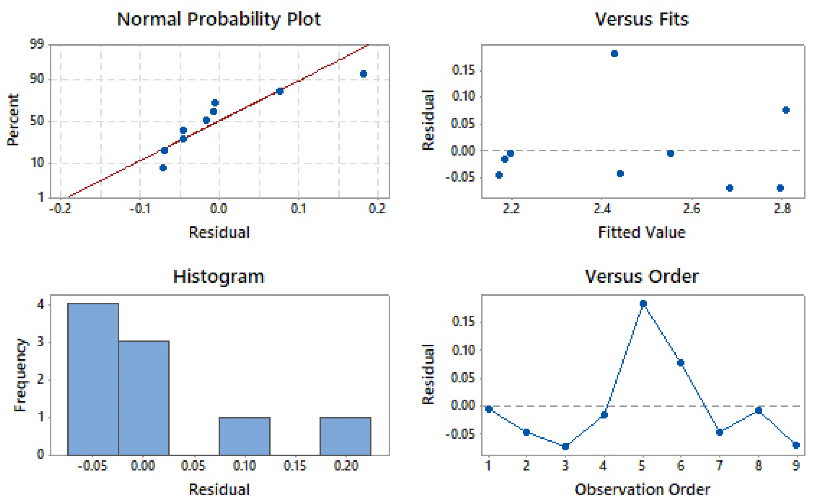
• The residual plots for all response variables verified the fitness of the proposed model for achieving a better future outcome. The significance of the machining parameters for each response was analyzed using contour plots.
• A difference of less than 20% between the values of R-sq. and Adj. R-sq. was observed for all responses, suggesting that the proposed models achieve the best fit for the existing data.
• Single-objective optimization results revealed the optimal process parameter settings—maximized MRR (3.738 g/s) and minimized SR (5.13 μm)—to be obtained at a laser power of 3000 W, a cutting speed of 8 m/min and a gas pressure of 6 bar.
• Single-objective optimization results demonstrated that the optimized process parameter settings achieving the minimum values of kerf width (296.384 μm) and dross height (0.1661 mm) were a laser power of 1000 W, a cutting speed of 8 m/min, and a gas pressure of 6 bar.
• Simultaneous-objective optimization results showed that a maximum MRR of 3.654 g/s, a minimum SR of 5.25 μm, a minimum kerf width of 302.839 μm, and a minimum dross height of 0.1684 mm could be obtained at a laser power of 1742 W, a cutting speed of 8 m/min, and a gas pressure of 6 bar.
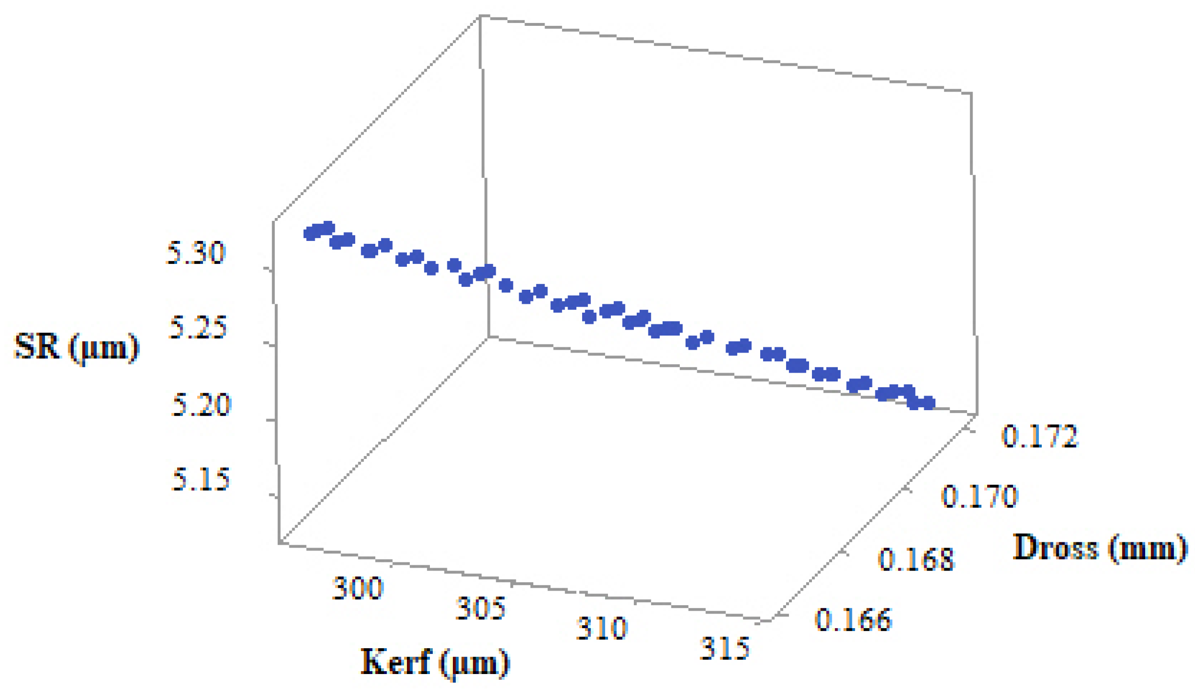
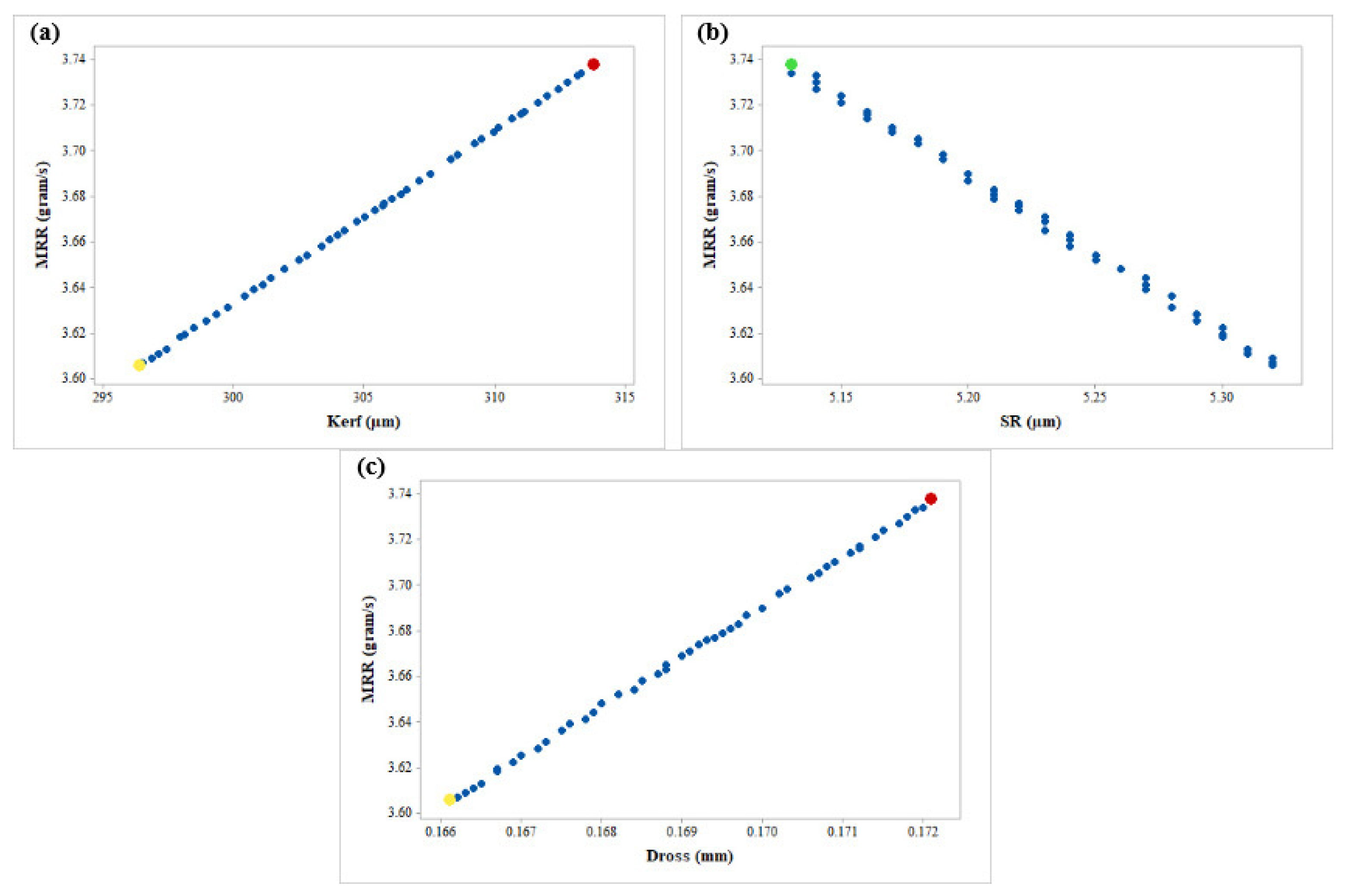
• The MOHTS algorithm was used to generate 49 non-dominant Pareto optimal points for all output responses. All these points provide optimum solutions for SR, kerf, dross, and MRR for individual input variables. Additionally, 3D and 2D Pareto curves were generated to allow better understanding by users.
• A negligible difference was observed between experimentally measured values and the predicted values of the HTS algorithm. This confirms that the existing HTS algorithm in addition to the proposed model is highly capable of and suitable for fiber laser cutting of Ti6Al4V.

References

1. Narutaki, N.; Murakoshi, A.; Motonishi, S.; Takeyama, H. Study on Machining of Titanium Alloys. CIRP Ann. 1983, 32, 65–69. [Google Scholar] [CrossRef]
2. Pramanik, A. Problems and solutions in machining of titanium alloys. Int. J. Adv. Manuf. Technol. 2014, 70, 919–928. [Google Scholar] [CrossRef]
3. Chaudhari, R.; Vora, J.; Parikh, D.M.; Wankhede, V.A.; Khanna, S. Multi-response Optimization of WEDM Parameters Using an Integrated Approach of RSM–GRA Analysis for Pure Titanium. J. Inst. Eng. India Ser. D 2020, 101, 117–126. [Google Scholar] [CrossRef]
4. Rahman, M.; Wang, Z.G.; Wong, Y.S. A review on high-speed machining of titanium alloys. JSME Int. J. Ser. C Mech. Syst. Mach. Elem. Manuf. 2006, 49, 11–20. [Google Scholar] [CrossRef] [Green Version]
5. Oke, S.R.; Ogunwande, G.S.; Onifade, M.; Aikulola, E.; Adewale, E.D.; Olawale, O.E.; Ayodele, B.E.; Mwema, F.; Obiko, J.; Bodunrin, M.O. An overview of conventional and non-conventional techniques for machining of titanium alloys. Manuf. Rev. 2020, 7, 34. [Google Scholar] [CrossRef]
6. Cadena, N.L.; Cue-Sampedro, R.; Siller, H.R.; Arizmendi-Morquecho, A.M.; Rivera-Solorio, C.; Di-Nardo, S. Study of PVD AlCrN Coating for Reducing Carbide Cutting Tool Deterioration in the Machining of Titanium Alloys. Materials 2013, 6, 2143–2154. [Google Scholar] [CrossRef] [Green Version]
7. Samodurova, M.; Logachev, I.; Shaburova, N.; Samoilova, O.; Radionova, L.; Zakirov, R.; Pashkeev, K.; Myasoedov, V.; Trofimov, E. A Study of the Structural Characteristics of Titanium Alloy Products Manufactured Using Additive Technologies by Combining the Selective Laser Melting and Direct Metal Deposition Methods. Materials 2019, 12, 3269. [Google Scholar] [CrossRef] [PubMed] [Green Version]
8. Fu, C.; Liu, J.; Guo, A. Statistical characteristics of surface integrity by fiber laser cutting of Nitinol vascular stents. Appl. Surf. Sci. 2015, 353, 291–299. [Google Scholar] [CrossRef]
9. Scintilla, L.D.; Sorgente, D.; Tricarico, L. Experimental Investigation on Fiber Laser Cutting of Ti6Al4V Thin Sheet. In Advanced Materials Research; Trans Tech Publications Ltd.: Bäch, Switzerland, 2011; Volume 264, pp. 1281–1286. [Google Scholar] [CrossRef]
10. Levichev, N.; Rodrigues, G.C.; Vorkov, V.; Duflou, J.R. Coaxial camera-based monitoring of fiber laser cutting of thick plates. Opt. Laser Technol. 2021, 136, 106743. [Google Scholar] [CrossRef]
11. Sheth, M.; Gajjar, K.; Jain, A.; Shah, V.; Patel, H.; Chaudhari, R.; Vora, J. Multi-objective Optimization of Inconel 718 Using Combined Approach of Taguchi—Grey Relational Analysis. In Advances in Mechanical Engineering; Springer: New York, NY, USA, 2020; pp. 229–235. [Google Scholar] [CrossRef]
12. Rathi, P.; Ghiya, R.; Shah, H.; Srivastava, P.; Patel, S.; Chaudhari, R.; Vora, J. Multi-response optimization of Ni55. 8Ti shape memory alloy using taguchi-grey relational analysis approach. In Recent Advances in Mechanical Infrastructure; Springer: Singapore, 2020; pp. 13–23. [Google Scholar]
13. Pimenov, D.Y.; Mia, M.; Gupta, M.K.; Machado, A.R.; Tomaz, Í.V.; Sarikaya, M.; Wojciechowski, S.; Mikolajczyk, T.; Kaplonek, W. Improvement of machinability of Ti and its alloys using cooling-lubrication techniques: A review and future prospect. J. Mater. Res. Technol. 2021, 11, 719–753. [Google Scholar] [CrossRef]
14. Chandrashekarappa, P.G.M.; Kumar, S.; Jagadish; Pimenov, D.Y.; Giasin, K. Experimental Analysis and Optimization of EDM Parameters on HcHcr Steel in Context with Different Electrodes and Dielectric Fluids Using Hybrid Taguchi-Based PCA-Utility and CRITIC-Utility Approaches. Metals 2021, 11, 419. [Google Scholar] [CrossRef]
15. Chaudhari, R.; Vora, J.J.; Prabu, S.S.M.; Palani, I.A.; Patel, V.; Parikh, D.M. Pareto optimization of WEDM process parameters for machining a NiTi shape memory alloy using a combined approach of RSM and heat transfer search algorithm. Adv. Manuf. 2019, 9, 64–80. [Google Scholar] [CrossRef]
16. Abbas, A.T.; Pimenov, D.Y.; Erdakov, I.; Mikolajczyk, T.; El Danaf, E.A.; Taha, M.A. Minimization of turning time for high-strength steel with a given surface roughness using the Edgeworth–Pareto optimization method. Int. J. Adv. Manuf. Technol. 2017, 93, 2375–2392. [Google Scholar] [CrossRef]
17. Abbas, A.T.; Pimenov, D.Y.; Erdakov, I.N.; Mikolajczyk, T.; Soliman, M.S.; El Rayes, M.M. Optimization of cutting conditions using artificial neural networks and the Edgeworth-Pareto method for CNC face-milling operations on high-strength grade-H steel. Int. J. Adv. Manuf. Technol. 2019, 105, 2151–2165. [Google Scholar] [CrossRef] [Green Version]
18. Patel, V.; Savsani, V. Heat transfer search (HTS): A novel optimization algorithm. Inf. Sci. 2015, 324, 217–246. [Google Scholar] [CrossRef]
19. Chaudhari, R.; Vora, J.J.; Prabu, S.S.M.; Palani, I.A.; Patel, V.K.; Parikh, D.M.; De Lacalle, L.N.L. Multi-Response Optimization of WEDM Process Parameters for Machining of Superelastic Nitinol Shape-Memory Alloy Using a Heat-Transfer Search Algorithm. Materials 2019, 12, 1277. [Google Scholar] [CrossRef] [Green Version]
20. Kratky, A.; Schuöcker, D.; Liedl, G. Processing with kW fibre lasers: Advantages and limits. In XVII International Symposium on Gas Flow, Chemical Lasers, and High-Power Lasers; International Society for Optics and Photonics: Lisboa, Portugal, 2008; p. 71311X. [Google Scholar] [CrossRef]
21. Powell, J.; Kaplan, A.F.H. A technical and commercial comparison of fiber laser and CO2 laser cutting. In International Congress on Applications of Lasers & Electro-Optics; Laser Institute of America: Chicago, IL, USA, 2012; pp. 277–281. [Google Scholar] [CrossRef]
22. Sołtysiak, R.; Wasilewski, P.; Sołtysiak, A.; Troszyński, A.; Maćkowiak, P. The Analysis of Fiber and CO2 Laser Cutting Accuracy. MATEC Web Conf. 2019, 290, 03016. [Google Scholar] [CrossRef]
23. El Aoud, B.; Boujelbene, M.; Bayraktar, E.; Salem, S.B.; Miskioglu, I. Studying effect of CO2 laser cutting parameters of titanium alloy on heat affected zone and kerf width using the Taguchi method. In Mechanics of Composite and Multi-Functional Materials; Springer: Cham, Switzerland, 2018; Volume 6, pp. 143–150. [Google Scholar]
24. Boudjemline, A.; Boujelbene, M.; Bayraktar, E. Surface Quality of Ti-6Al-4V Titanium Alloy Parts Machined by Laser Cutting. Eng. Technol. Appl. Sci. Res. 2020, 10, 6062–6067. [Google Scholar] [CrossRef]
25. Scintilla, L.; Palumbo, G.; Sorgente, D.; Tricarico, L. Fiber laser cutting of Ti6Al4V sheets for subsequent welding operations: Effect of cutting parameters on butt joints mechanical properties and strain behaviour. Mater. Des. 2013, 47, 300–308. [Google Scholar] [CrossRef]
26. Scintilla, L.D.; Tricarico, L. Fusion cutting of aluminum, magnesium, and titanium alloys using high-power fiber laser. Opt. Eng. 2013, 52, 076115. [Google Scholar] [CrossRef]
27. Manjoth, S.; Keshavamurthy, R.; Kumar, G.S.P. Optimization and Analysis of Laser Beam Machining Parameters for Al7075-TiB2In-situ Composite. IOP Conf. Ser. Mater. Sci. Eng. 2016, 149, 012013. [Google Scholar] [CrossRef]
28. Poshyananda, V.; Darayen, J.; Tumkhanon, K.; Puncreobutr, C.; Khamkongkaeo, A.; Lohwongwatana, B. Consideration of key process parameters for achieving robust and uniform cutting of Ti-6Al-4V sheet metal using fiber laser with nitrogen assisted gas. J. Met. Mater. Miner. 2018, 28. [Google Scholar]
29. Fu, C.H.; Guo, Y.B. Laser cutting simulation of nitinol stent alloy with moving heat flux. In Proceedings of the International Conference on Shape Memory and Superelastic Technologies American Society for Metals, Pacific Grove, CA, USA, 12–16 May 2014. [Google Scholar]
30. Shanjin, L.; Yang, W. An investigation of pulsed laser cutting of titanium alloy sheet. Opt. Lasers Eng. 2006, 44, 1067–1077. [Google Scholar] [CrossRef]
31. Pandey, A.K.; Dubey, A.K. Simultaneous optimization of multiple quality characteristics in laser cutting of titanium alloy sheet. Opt. Laser Technol. 2012, 44, 1858–1865. [Google Scholar] [CrossRef]
32. Andersson, N.; Granberg, C. Laser Cutting in Ti6Al4V Sheet: DOE and Evaluation of Process Parameters Informative. Master’s Thesis, Department of Materials and Manufacturing Technology, Chalmers University of Technology, Gothenburg, Sweden, 2015. [Google Scholar]
33. Yilbas, B.S.; Akhtar, S.S.; Keles, O. Laser straight cutting of Ti-6Al-4V alloy: Temperature and stress fields. In Materials and Surface Engineering; Woodhead Publishing: Sawston, UK, 2012; pp. 243–265. [Google Scholar] [CrossRef]
34. Reck, A.; Zeuner, A.T.; Zimmermann, M. Fatigue Behavior of Non-Optimized Laser-Cut Medical Grade Ti-6Al-4V-ELI Sheets and the Effects of Mechanical Post-Processing. Metals 2019, 9, 843. [Google Scholar] [CrossRef] [Green Version]
35. Yilbas, B.S. The Laser Cutting Process. Analysis and Applications; Elsevier Science: San Diego, CA, USA, 2017. [Google Scholar]
36. da Silva, P.S.C.P.; Campanelli, L.C.; Escobar Claros, C.A.; Ferreira, T.; Oliveira, D.P.; Bolfarini, C. Prediction of the surface finishing roughness e_ect on the fatigue resistance of Ti-6Al-4V ELI for implants applications. Int. J. Fatigue 2017, 103, 258–263. [Google Scholar] [CrossRef]
37. Farooq, M.U.; Mughal, M.P.; Ahmed, N.; Mufti, N.A.; Al-Ahmari, A.M.; He, Y. On the Investigation of Surface Integrity of Ti6Al4V ELI Using Si-Mixed Electric Discharge Machining. Materials 2020, 13, 1549. [Google Scholar] [CrossRef] [Green Version]
38. Chaurasia, A.; Wankhede, V.A.; Chaudhari, R. Experimental Investigation of High-Speed Turning of INCONEL 718 Using PVD-Coated Carbide Tool Under Wet Condition. In Innovations in Infrastructure; Springer: Singapore, 2019; pp. 367–374. [Google Scholar] [CrossRef]
39. Chaudhari, R.; Vora, J.J.; Pramanik, A.; Parikh, D. Optimization of Parameters of Spark Erosion Based Processes. In Spark Erosion Machining; CRC Press: Boca Raton, FL, USA, 2020; pp. 190–216. [Google Scholar] [CrossRef]
40. Chaudhari, R.; Vora, J.J.; Patel, V.; de Lacalle, L.N.L.; Parikh, D.M. Surface Analysis of Wire-Electrical-Discharge-Machining-Processed Shape-Memory Alloys. Materials 2020, 13, 530. [Google Scholar] [CrossRef] [Green Version]
41. Rao, B.T.; Kaul, R.; Tiwari, P.; Nath, A. Inert gas cutting of titanium sheet with pulsed mode CO2 laser. Opt. Lasers Eng. 2005, 43, 1330–1348. [Google Scholar] [CrossRef]
42. Kliner, D.A.V.; Chong, K.; Franke, J.; Gordon, T.D.; Gregg, J.; Gries, W.; Hu, H.; Ishiguro, H.; Issier, V.; Kharlamov, B.; et al. 4-kW fiber laser for metal cutting and welding. In Fiber Lasers VIII: Technology, Systems, and Applications; International Society for Optics and Photonics: San Francisco, CA, USA, 2011; Volume 7914, p. 791418. [Google Scholar] [CrossRef]
43. Chaudhari, R.; Vora, J.; Lacalle, L.N.; Khanna, S.; Patel, V.K.; Ayesta, I. Parametric Optimization and Effect of Nano-Graphene Mixed Dielectric Fluid on Performance of Wire Electrical Discharge Machining Process of Ni55. 8Ti Shape Memory Alloy. Materials 2021, 14, 2533. [Google Scholar] [CrossRef]
44. O’Neill, W.; Sparkes, M.; Varnham, M.; Horley, R.; Birch, M.; Woods, S.; Harker, A. High power high brightness industrial fiber laser technology. In International Congress on Applications of Lasers & Electro-Optics; Laser Institute of America: Chicago, IL, USA, 2004; Volume 2004, p. 301. [Google Scholar]
45. Sharma, V.; Kumar, V.; Bist, A. Investigations on morphology and material removal rate of various MMCs using CO2 laser technique. J. Braz. Soc. Mech. Sci. Eng. 2020, 42, 1–14. [Google Scholar] [CrossRef]
46. Chaudhari, R.; Vora, J.J.; Patel, V.; De Lacalle, L.N.L.; Parikh, D.M. Effect of WEDM Process Parameters on Surface Morphology of Nitinol Shape Memory Alloy. Materials 2020, 13, 4943. [Google Scholar] [CrossRef] [PubMed]
Figure 1. (a) SR measurement; (b) kerf measurement; (c) dross measurement.
Metals 11 01461 g001
Figure 2. Percentage contribution of machining variables on SR.
Metals 11 01461 g002
Figure 3. Impact of machining variables on SR.
Metals 11 01461 g003
Figure 4. Residual plots for SR.
Metals 11 01461 g004
Figure 5. Contour plot of SR.
Metals 11 01461 g005
Figure 6. Percentage contribution of machining variables on kerf width.
Metals 11 01461 g006
Figure 7. Impact of machining variables on kerf.
Metals 11 01461 g007
Figure 8. Residual plots for kerf.
Metals 11 01461 g008
Figure 9. Contour plot of kerf.
Metals 11 01461 g009
Figure 10. Percentage contribution of machining variables on dross.
Metals 11 01461 g010
Figure 11. Impact of machining variables on dross.
Metals 11 01461 g011
Figure 12. Residual plots for dross.
Metals 11 01461 g012
Figure 13. Contour plot of dross.
Metals 11 01461 g013
Figure 14. Percentage contribution of machining variables to MRR.
Metals 11 01461 g014
Figure 15. Impact of machining variables on MRR.
Metals 11 01461 g015
Figure 16. Residual plots for MRR.
Metals 11 01461 g016
Figure 17. Contour plot of MRR.
Metals 11 01461 g017
Figure 18. Flow chart of the heat transfer search (HTS) algorithm [18].
Metals 11 01461 g018
Figure 19. 3D Pareto curve of SR vs. Dross vs. Kerf.
Metals 11 01461 g019
Figure 20. 2D Pareto curve of (a) MRR vs. Kerf, (b) MRR vs. SR, (c) MRR vs. Dross.
Metals 11 01461 g020