Multi-Objective Optimization of Performance Indicators in Turning of AISI 1045 under Dry Cutting Conditions

Abstract

In machining operations, minimizing the usage of resources such as energy, tools, costs, and production time, while maximizing process outputs such as surface quality and productivity, has a significant impact on the environment, process sustainability, and profit. In this context, this paper reports on the utilization of advanced multi-objective algorithms for the optimization of turning-process parameters, mainly cutting speed, feed rate, and depth of cut, in the dry machining of AISI 1045 steel for high-efficient process. Firstly, a number of experimental tests were conducted in which cutting forces and cutting temperatures are measured. Then the material removal rate and the obtainable surface roughness were determined for the examined range of cutting parameters. Next, regression models were developed to formulate the relationships between the process parameters and the four process responses. After that, four different multi-objective optimization algorithms, (1) Gray Wolf Optimizer (GWO) and (2) Weighted Value Gray Wolf Optimizer (WVGWO), (3) Multi-Objective Genetic Algorithm (MOGA), and (4) Multi-Objective Pareto Search Algorithm (MOPSA), were applied. The results reveal that the optimal running conditions of the turning process of AISI 1045 steel obtained by WVGWO are a feed rate of 0.050 mm/rev, cutting speed of 156.5 m/min, and depth of cut of 0.57 mm. These conditions produce a high level of material removal rate of 4460.25 mm³/min, in addition to satisfying the surface quality with a roughness average of 0.719 µm. The optimal running conditions were found to be dependent on the objective outcomes’ order. Moreover, a comparative evaluation of the obtainable dimensional accuracy in both dry and wet turning operations was carried out, revealing a minimal relative error of 0.053% maximum between the two turning conditions. The results of this research work assist in obtaining precise, optimal, and cost-effective machining solutions, which can deliver a high-throughput, controllable, and robust manufacturing process when turning AISI 1045 steel.

1. Introduction

As modern industry increasingly transforms manufacturing into highly automated systems, condition monitoring, process modeling, and optimization become more and more important. Manufacturers with access to better predictors and optimizers of the manufacturing processes have an edge over their competitors [1]. Process optimization is very important for manufacturing processes, as it improves efficiency in terms of process economics and product quality [2]. For example, in the machining of component parts, cutting parameters constitute the process variables to be optimized in order to simultaneously minimize cost and consumed energy, while improving product quality and maximizing the productivity at the same time. Given their high ability as a dependable means to tackle complex non-linear processes, artificial-intelligence techniques have been widely utilized to model and optimize machining operations [3].

A recent review presented a new approach that divides the turning-process energy into two categories: the electrical energy consumed by the machine tool, and the embodied energy of cutting tool and cutting fluid [4]. To support this point of view, it utilizes results from other works to introduce a number of optimal cutting conditions. These cutting conditions of turning operations, which are usually the subject of optimization by different researchers, include the cutting speed ($v_c$) in m/min, the feed rate ($f_r$) in mm/rev, and the depth of cut ($a_p$) in mm. Recently, the tool geometry has also been under focus as a cutting parameter [5,6]. A thorough study used Response Surface Method (RSM) and Analysis of Variance (ANOVA) to develop a model for the prediction of surface roughness and temperature based on the three main cutting parameters, namely cutting speed, feed rate, and depth of cut, with the target of relating surface roughness and work piece temperature as dependent variables to cutting parameters as decision variables [7]. Moreover, by means of RSM, a multicriteria optimization model was developed in order to enhance the surface roughness and vibration during the turning of AISI 5140 steel. This optimization model targeted the cutting speed ($v_c$), feed rate ($f_r$), and cutting edges angles ($\kappa$) that led to the optimum parameters at $v_c$ = 190 m/min, $f_r$ = 0.06 mm/rev, and $\kappa$ = 60° [8]. The depth of cut was found to bear a strong effect on the surface temperature of the work piece. Direct proportionality was detected between the feed rate and surface roughness, while the opposite was found with surface temperature, which was inversely proportional to the feed rate. Another study involved the influence flank wear in addition to the three main turning parameters: feed rate, cutting speed, and depth of cut on the resulting cutting forces and surface roughness [9]. It revealed that the tangential cutting force was sensitively dependent on the depth of cut. It also stated that surface roughness was found to depend on the variation of the feed rate. Interestingly, the study deduced that the flank wear has a noticeable effect on surface roughness and the process cutting forces. An experimental and statistical study on the turning operations of aluminum in dry conditions also addressed the influence of the surface roughness and cutting forces [10]. The parameter with the highest effect on surface roughness was the feed rate, with more than a 70% contribution. The cutting speed and depth of cut had less contribution. The resulting cutting forces were influenced primarily by one single parameter, which is the depth of cut, with almost 9.0% contribution. In addition, it was reported that the proposed prediction models achieved a mean absolute error of 3.47% for surface roughness and 6.8% for the cutting forces. The work introduced an artificial neural network model (ANN) to validate the regression model used to predict surface roughness and cutting forces. The model prediction of surface roughness and cutting forces had acceptable accuracy.

Another parameter that may contribute to the variation of cutting forces or consumed energy is the specific material of the cutting tool. This was investigated by Hernández-González et al. [11], who used CT5015-P10 and GC4225-P25 inserts and different cutting speeds to monitor forces and specific energy consumption (SEC) in the dry high-speed turning of AISI 1045 steel. They compared cutting forces measured from experiments with predicted results from the proposed models. The comparison criteria included two performance metrics: coefficient of determination and root mean square error (RMSE). It was found that the polynomial models showed a lack of regression, as the R-squared value was less than 70%. The cutting speeds and machining times associated with extreme values of SEC for both tool inserts were calculated. The results showed that the lowest SEC values were obtained at a medium cutting speed. Moreover, the SEC for the GC4225 insert was found to be higher than that for the CT5015 tool. Dhar et al. [12] investigated the turning of AISI 1060 steel, using carbide inserts to evaluate the effects of using high-pressure coolant on different process parameters, including cutting temperature, chip types, cutting forces, tool wear and life, and surface finish. Moreover, Kuntoğlu et al. [13] used chemical-vapor-deposition-coated carbide inserts with different levels of hardness in the turning of AISI 1050. The surface roughness, tool wear, and acoustic emissions were investigated carefully. Finally, for better machinability, the hardness of the cutting tools was recommended to be between 60 and 70 HRC.

Understandably, using a high-pressure coolant during cutting noticeably reduced cutting forces and tool wear and produced improved surface roughness. Another favorable result is that the tool life was remarkably extended because the temperature within the cutting zone was considerably lower. Chip–tool and work–tool interactions have also been improved. The effects of the turning-process conditions on cutting-tool temperature and surface roughness for both dry conditions were studied. For both cases, the most prominent factors were found to be the depth of cut and cutting speed. When fixing cutting parameters, the cutting-tool minimum temperature was 59 °C for the case of dry operation, and 32 °C for the case of coolant operation. A cutting-tool maximum temperature of 110 °C was attained with higher cutting parameters. The effects of changing the three parameters, depth of cut, cutting speed, and feed rate on the cutting-tool temperature varied. The effect of the first two were more prominent than the latter. The sequence of significance is as follows: first the cutting speed, then the depth of cut, and lastly the feed rate. Interestingly, the surface roughness greatly improved when the depth of cut was reduced but the cutting seed was increased [14].

The effects of the dry machining of Ti6Al4V on the surface integrity of machined work piece were investigated. The driving motive was to detect changes occurring in subsurface deformation when changing cutting speed and feed rate while keeping fixed depth of cut. Damage on the machined edge of the work piece was induced by deformations resulting from restructuring of microstructure, with a correlation to the chip microstructure. Furthermore, at higher cutting parameters, the thermal softening phenomenon became more dominant. This resulted in a higher surface roughness, lower microhardness values beneath the surface, and a coarser microstructure when using high cutting parameters. The chip microstructure validated the thermal softening and work-hardening phenomenon. A further microstructure analysis showed that high cutting speeds and feed rate increase the shear band formation and frequency of chip segmentation. However, using lower cutting parameters reduced segmentation frequency and increased deformed grains around shear bands [15]. With the aim of controlling the thermal softening of the material during heavy-duty machining, He et al. [16] investigated the main cause of shear fracture of 2.25Cr-1Mo-0.25V steel. It is found that an elevated temperature can affect the shear flow on the machining region, hence softening the steel workpiece.

Numerous optimization techniques were introduced to improve the turning process. Until recently, the turning output parameters that are mostly under analysis were the surface roughness, material removal rate, and cutting-tool life [17]. However, many researchers started to investigate the effect of process running conditions on new outcomes, such as machine tool power consumption [18], cutting forces, and temperature, among others. As the number of outcomes under analysis increases the more the need for evolutionary multi-objective optimization techniques increases. The optimization techniques are categorized into many types as follows: the nature-inspired and population-based metaheuristics, trajectory-based and graph-based algorithms, and the machine-learning and deep-learning methods. In this research, the multi-objective genetic algorithm (MOGA) was used as the population-based algorithm, the gray wolf multi-objective optimizer (GWO) [19] and improved gray wolf optimizer using weighted values (WVGWO) [20] were used as nature-inspired metaheuristics, and multi-objective pareto search algorithm (MOPSA) was used as the graph-based algorithm. The two latter algorithms showed superior performance in many benchmark problems and compared to many known algorithms, such as simulated annealing (SA), particle swarm optimizer (PSO), evolutionary algorithm base on decomposition (EA/D), and even the genetic algorithm (GA) [19].

Recently, an optimization study addressed the optimal turning parameters to the reduce surface roughness while turning by high-speed steel-cutting tool, using the Taguchi method [21]. It concluded that cooling affects surface roughness quality remarkably by contributing about one-half of the total effect, and the feed rate accounts for about one-fourth. The results from the optimization technique showed that a minimum surface roughness is achieved with a cutting speed of 60 m/min, a depth of cut of 0.1 mm, and a feed rate of 0.05 mm/rev under minimum quantity lubricant (MQL) condition. Meanwhile, a deep investigation and optimization on the turning process of AISI 1050 under (MQL) was carried out by using Taguchi’ method and RSM methodology. The optimization results were MQL at 120 mL/h, speed of cut = 200 m/min, feed rate = 0.07 mm/rev, and depth of cut = 1.2 mm [22]. Another study included effects of varying insert-tool-nose radii on the surface quality and cutting forces for EN 10,503 steel alloy. It used a combination of Taguchi and VIKOR methods. The result of optimization gave values of $v_c$ = 78.62 m/min, $f_r$ = 0.08 mm/rev, and $a_p$ = 0.5 mm and an insert-nose radius of 0.4 mm. These cutting conditions resulted in desirable values of surface roughness of 0.621 μm, resultant cutting force of 360 N, and material removal rate (MRR) of 60,000 mm³/min [18]. Moreover, the effect of the cutting speed, feed rate, and tool tip on the tool wear and acoustic emissions was investigated, in addition to implementing a prediction sensor system for tool break. The optimal running conditions to obtain the minimum tool wear and achieve higher quality product are $v_c$ = 135 m/min, $f_r$ = 0.214 mm/rev, and tool tip of type P25 according to authors’ coding [23]. Furthermore, using Taguchi and ANOVA analysis, the most influential factor on the surface roughness of steel (1.2738) was the depth of cut. This resulted in the optimal cutting conditions of $v_c$ = 300 mm/min, $f_r$ = 0.3 mm/rev, and $a_p$ = 1 mm, which produced a surface roughness of 1.10 μm [24]. The effects of process parameters during machining of alloy steel AISI 1040 were analyzed by using RSM methodology. It was shown that the chip formation frequency is proportional directly to the depth of cut and indirectly to the cutting speed. The resulting optimal conditions were a cutting speed of 50 mm/s, feed rate of 0.8 ft/rev., and depth of cut of 0.79 mm [25]. Finally, a parametric optimization comparison on cutting forces and material removal rate of the turning of AISI 5140 showed that the Harmonic Artificial Bee Colony Algorithm and RSM outperformed the accuracy of the optimization results of Taguchi’s method and Harmonic Bee Colony at optimal running conditions of $v_c$ = 280 mm/min, $f_r$ = 0.18 mm/rev, and $a_p$= 1 mm [26]. The literature review regarding the optimization of the machining of different steel alloys is listed in

Table 1. List of research results in the literature.

No.	Material	Optimization Algorithm	${\mathit{v}}_{\mathit{c}}$ (m/min)	${\mathit{f}}_{\mathit{r}}$ (mm/rev)	${\mathit{a}}_{\mathit{p}}$ (mm)	Reference
1	AISI 5140	ANOVA a	190	0.06	-	[8]
2	SKD61	Taguchi	60	0.05	0.1	[21]
3	AISI 1050	Taguchi and RSM b	200	0.07	1.2	[22]
4	EN 10503	Taguchi and VIKOR	78.62	0.08	0.5	[18]
5	AISI 1050	ANOVA	135	0.214	-	[23]
6	AISI 1040	Taguchi and ANOVA	300	0.3	1	[24]
7	AISI 1040	RSM, TS and SA c	50 mm/s	0.80 ft/rot.	0.79	[25]
8	AISI 5140	RSM, H-ABC d and Taguchi	280	0.18	1	[26]

^a ANOVA, Analysis of Variance. ^b RSM, Response Surface Methodology. ^c TS, Tabu Search optimization; SA, simulated annealing. ^d H-ABC, Harmonic Artificial Bee Colony Algorithm.

.

Looking at the preceding reviewed literature, it is not difficult to see that a number of research works attempted experimentally to investigate the effects of changing turning operation parameters on a number of process outputs and the optimization of a single response or multiple responses, such as productivity, surface quality, tool wear, cutting forces, and temperature. Nevertheless, a challenge yet to be addressed is to employ more robust optimization techniques with multi-objective optimization tools to simultaneously identify proper cutting conditions for a number of machining responses for more precise, sustainable, high-throughput, and controllable machining processes [27]. In this context, this study aimed to conduct both an experimental investigation and multi-objective optimization tools for the concurrent identification of minimization of cutting forces, cutting temperature, and surface roughness, while maximizing process productivity during the turning of AISI 1045 in dry condition. The selection of dry condition while turning the AISI 1045 alloy is experimentally justified by showing that the difference in dimensional accuracy between wet and dry conditions can be neglected.

Following this introduction, the Materials and Methods section describes in depth the AISI 1045 steel alloy and tools used in this study. It illustrates the microstructure and mechanical properties of the material, the specifications of the machines and tools used in experiments, and the optimization techniques applied. Then the Results and Discussion section presents the results from both the experimental and computational investigations and provides a comparison between them, in addition to the multi-objective optimization of the turning process. Finally, the findings of this research work are presented at the end of the document.

2. Materials and Methods

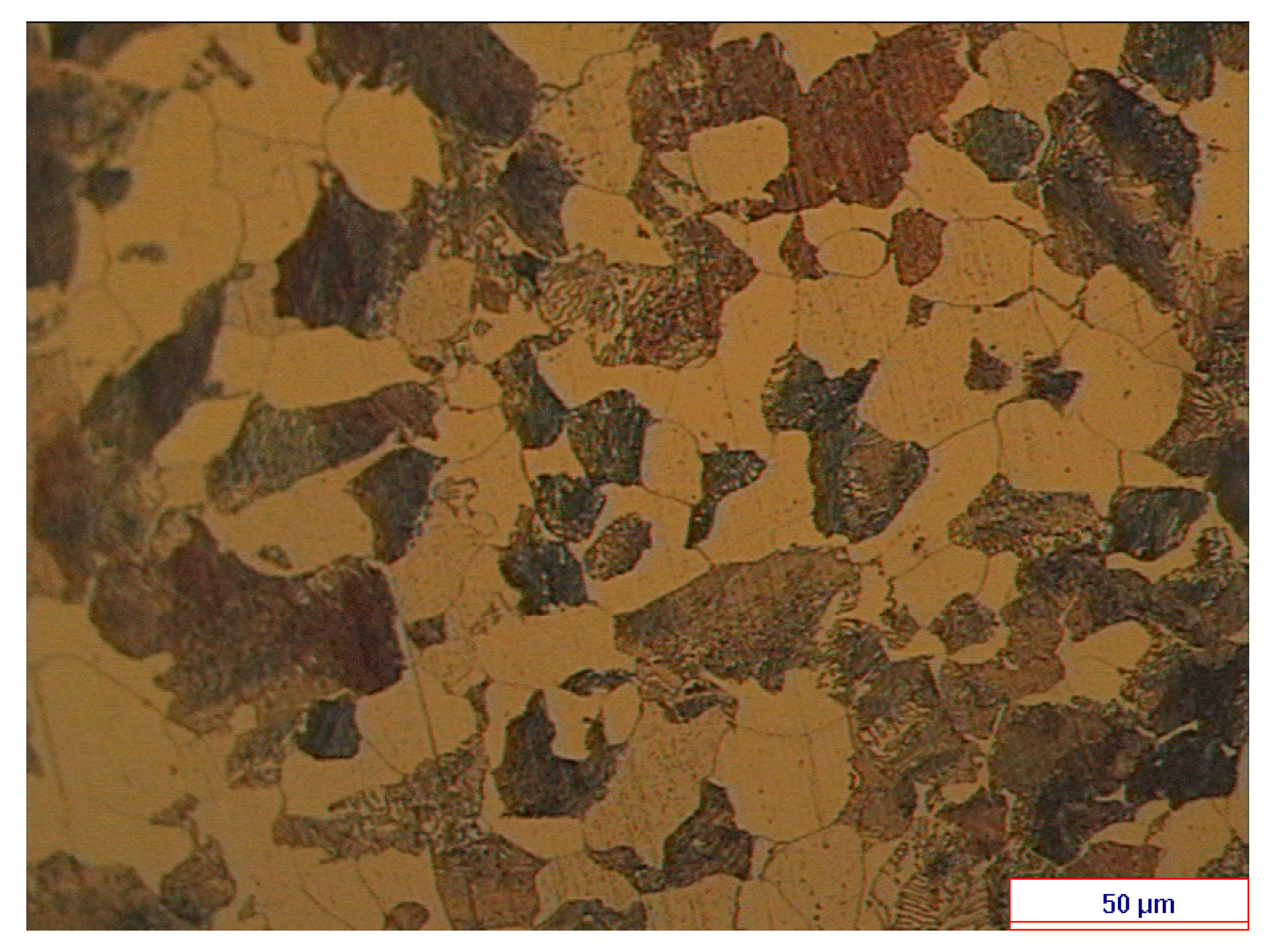
This section presents the experimental work conducted in this study. In particular, this section starts with a brief introduction to the material processed and its chemical composition, mechanical properties, and microstructure. Then the machining setup, entailing the computerized numerical control (CNC) machine, cutting tools, and characterization devices used, is provided. Next, the section reports the design of experiment followed to conduct the experimental trials. Finally, the optimization algorithms and their working envelope are presented in detail.

2.1. Materials

The material used in this analysis is AISI 1045 steel, which is widely used in most industrial applications requiring high wear resistance and strength. Typical applications of AISI 1045 include gears, shafts, spindles, rolls, and crankshafts. Moreover, AISI 1045 has good machinability in all machining operations, such as turning, milling, broaching, and drilling. The characteristics of this steel alloy are shown in

Table 2. Chemical compositions of AISI 1045.

Element	C	Fe	Mn	P	S
Percentage %	0.45	98.75	0.65	0.03	0.04

and

Table 3. Mechanical Properties of AISI 1045.

Properties	Value
Tensile Strength, Ultimate	565 MPa
Tensile Strength, Yield	310 MPa
Elongation at Break (in 50 mm)	16%
Reduction of Area	40%
Modulus of Elasticity (Typical for steel)	200 GPa
Hardness, Vickers	170

, where Table 2 shows its chemical composition, and Table 3 shows the mechanical properties.

Microstructure of the Material

For optical microscopy, the sample was prepared according to standard metallographic sample preparation, which includes grinding by using SiC sandpaper, then polishing with diamond paste of 1.0 μm, and finally etching with 5% Nital to reveal the sample’s microstructure. Figure 1 shows the microstructure of the material investigated in this work. As seen from the figure, the microstructure contains grains of pearlite (dark) in a matrix of ferrite (light). The pearlite grains contain alternate lamellas of proeutectoid ferrite (Fe) and cementite (Fe₃C) with random orientation and inter-lamellar spacing. The pearlite phase constituted 38% volume-fraction, whereas ferrite was 62%.

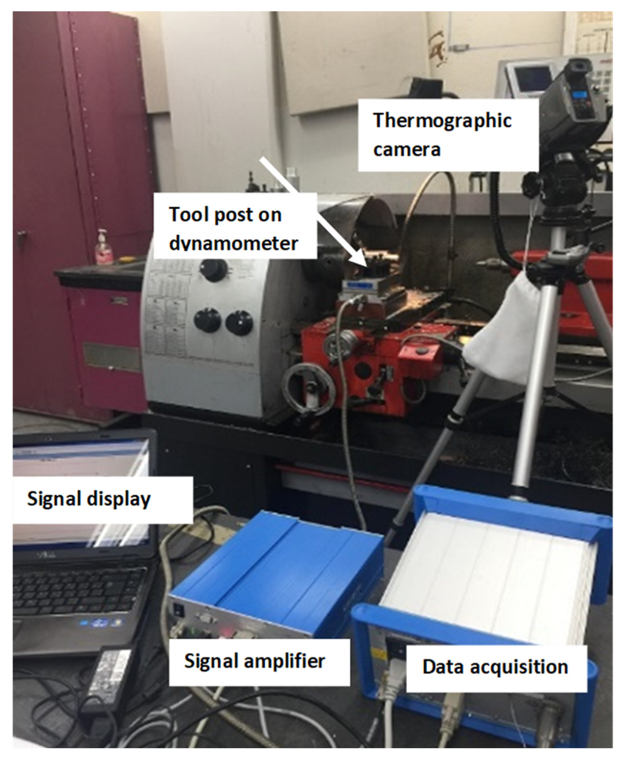
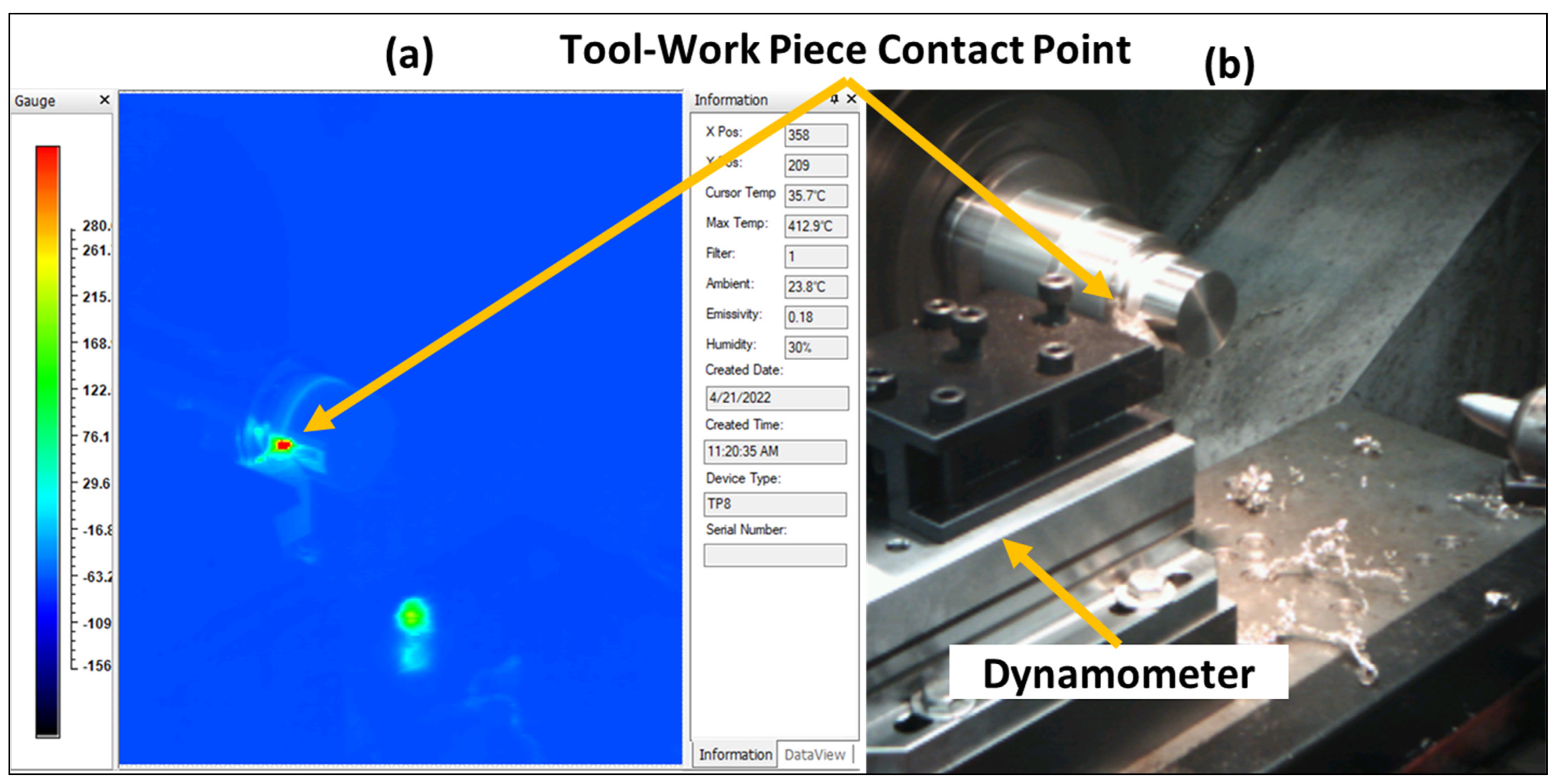
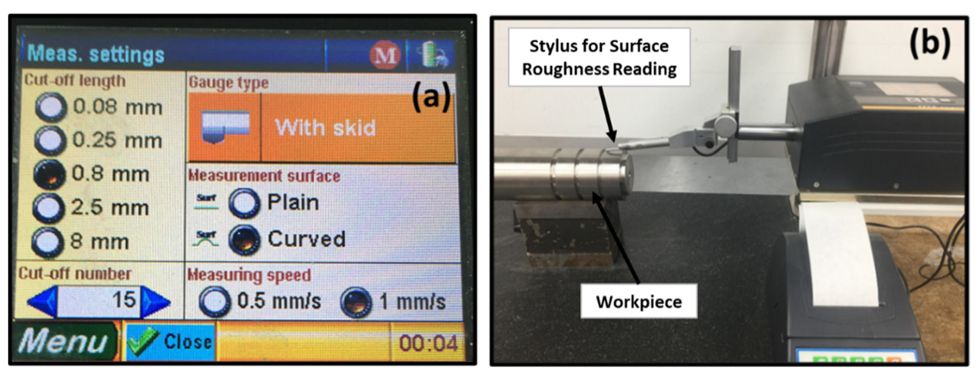
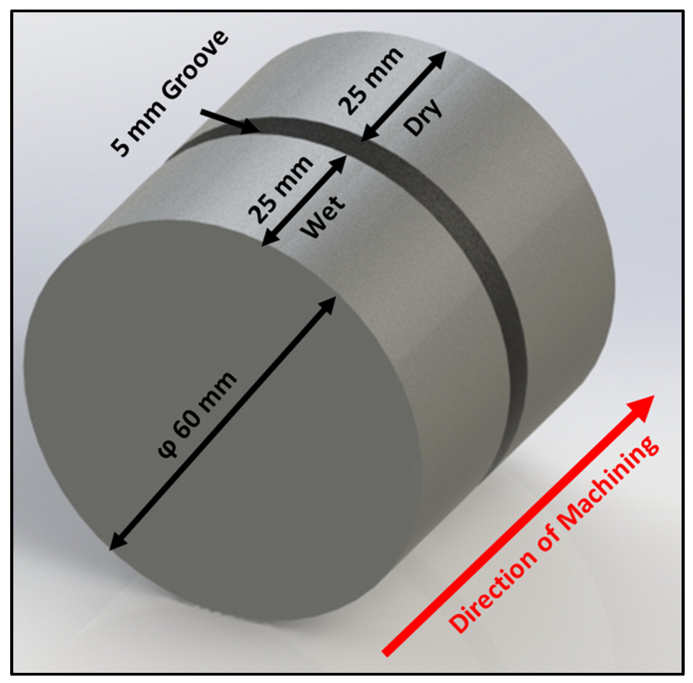
2.2. Machining Setup

A conventional turning machine type, EMCOMAT- 20D by Emco Company (Salzburg, Austria), was used for machining the test pieces. This machine has a permanent position display for the bed, cross slide, and top slide on the thin film transistor (TFT) screen. The position of the bed slide is monitored by a high-precision rack on the encoder. The position of the cross slide is measured by a glass scale with an accuracy of 0.001 mm. This allows diameters to be set with extremely high precision. The position of the top slide is measured by the direct driven encoder. Functions: constant cutting speed, 999 tools, 999 reference points, home position, remaining path, imperial/metric, radius/diameter display screen size of 6.5 color TFT, 640 × 480 (VGA). It has a 5.3 kW drive motor and electronic speed controls up to 3000 rpm. The longitudinal feed rate range is 0.045–0.787 mm/rev.

The cutting tool was manufactured by Sandvik (Stockholm, Sweden), with the following ordering code: holder type, SDJCR 2020K 11; and insert type, DCMT11 T304-PF 4315. This tool has the following specifications: insert shape angle = 55°, clearance angle = 7°, rake angle = 6°, and tool nose radius = 0.4 mm. This tool was designed for efficient material removal rates. It is commonly used for all types of materials, from stainless steel to titanium alloys. The workpiece has the following dimensions: length of 120 mm and diameter of 70 mm. The cut length for experiments is 30 mm for each run.

The test rig for the experimental work, comprising sets for the machining of test pieces, measurement of cutting forces, and measurement of the cutting temperature, is shown in Figure 2.

A dynamometer manufacturing by Kistler company type Kistler 5070 equipped with dynoware software type 2825A (Liechtenstein, Switzerland) was used for evaluating the three cutting forces: radial force ($F_r$), feed force ($F_f$), and main cutting force ($F_c$), as shown in Figure 3. Dubey et al. [28] selected the main cutting force to represent the cutting forces as an objective to be optimized. However, in this work, the the combination of the three forces’ vectors is considered to be more representable for the machine power consumption. All forces are measured in Newton (N). The resultant force (R) can be calculated from Equation (1):

$$\mathrm{R}=\sqrt{F_r{}^2+F_f{}^2+F_c{}^2}$$

(1)

A thermographic camera of the type ThermoPro-TP8, provided by Guide (Wuhan, China), was used to take the thermal images. The specifications of this camera are shown in

Table 4. ThermoPro-TP8 specifications.

Property	Reference
Thermal Sensitivity	≤0.08 °C at 30 °C
Measuring range	−20 °C–1000 °C
Detector type	Micro-bolometer UFPA384 × 288 pixels
Spectral Range	8~14 μm
Accuracy	± 2 °C
Emissivity	0.18

.

The stability and focus of the camera during imaging are very important. The camera performs auto calibration; however, manual calibrations are recommended before taking the needed images to ascertain that proper sensitivity is achieved that has to be stable and focused on the target of interest for which the temperature is to be measured. The camera has to be focused on the target, with the distance between them recorded and fed to the analysis software among the parameters used for temperature evaluation. In this experiment, the target of interest is the surface between the cutting edge of the tool and the workpiece during the machining operation, as shown in Figure 4; hence, the mean cutting temperature of this contact surface along the turning process was considered. The emissivity coefficient is determined from the manual table. The value of the coefficient depends on the material type, the surface condition (roughness), the temperature to be measured, the angle of view, and the wavelength.

A surface-tester-type Rugosurf 90-G, from Tesa (Bugnon, Switzerland) was used to measure the surface roughness, Ra. The settings of measurement parameters are cutoff length of 0.8 mm and measuring speed of 1 mm/s, as shown in Figure 5.

2.3. Design of Experiment

A full factorial design of experiment 3³ was set with 27 tests run as the following: three levels of each parameter—cutting speed of 80, 120, and 160 m/min; depth of cut 0.5, 0.75, and 1.0 mm; and feed rate 0.045, 0.09, and 0.135 mm/rev, as shown in

Table 5. Running-condition parameters and their levels.

Parameter	Levels
Cutting speed ($v_c$)	[80 120 160] m/min
Depth of cut ($a_p$)	[0.5 0.75 1] mm
feed rate ($f_r$)	[0.045 0.09 0.135] mm/rev

. The desired outputs are 4 objectives: surface roughness (Ra) in μm, the resultant cutting force (R) in N, the cutting temperature (T) in °C, and the material removal rate (MRR) in mm³/min. Finally, each test was repeated three times, and the average results were considered.

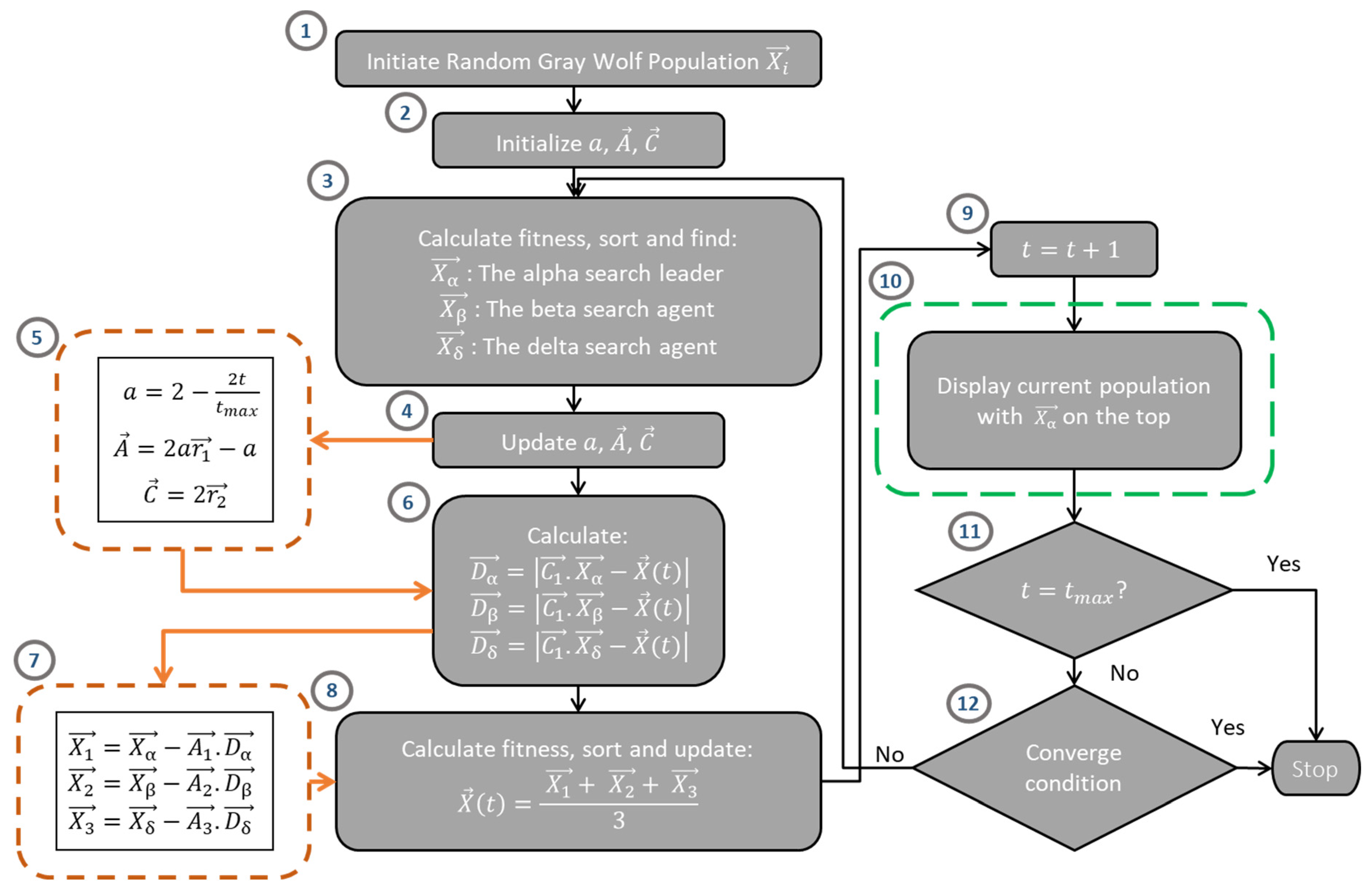
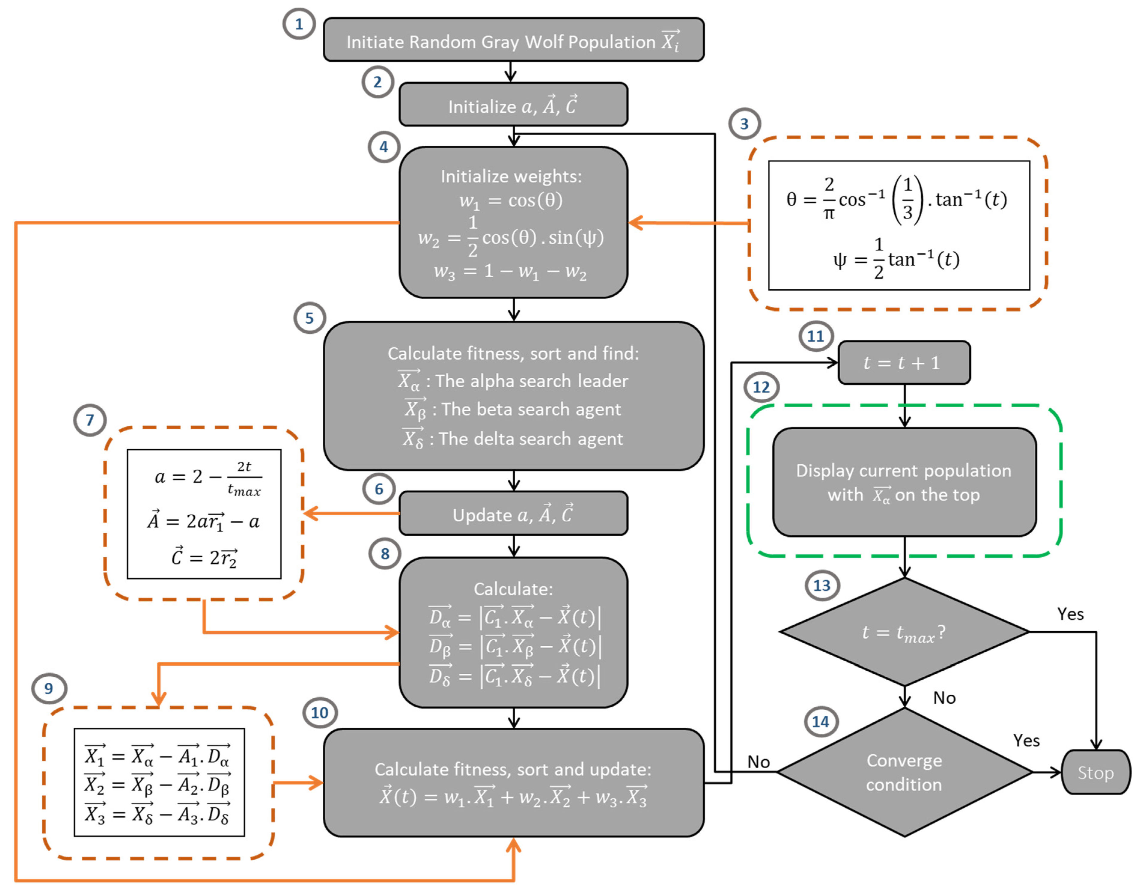
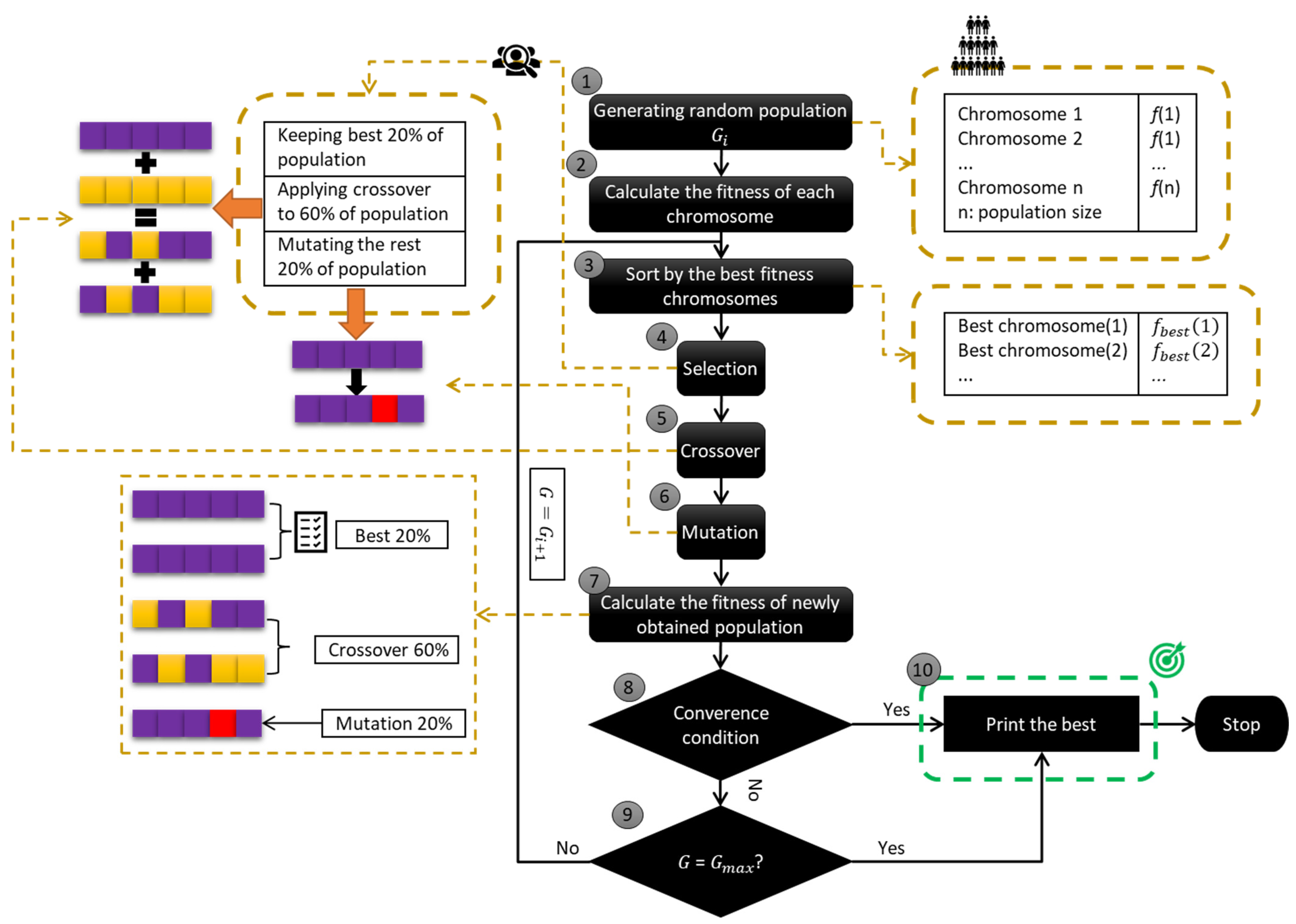
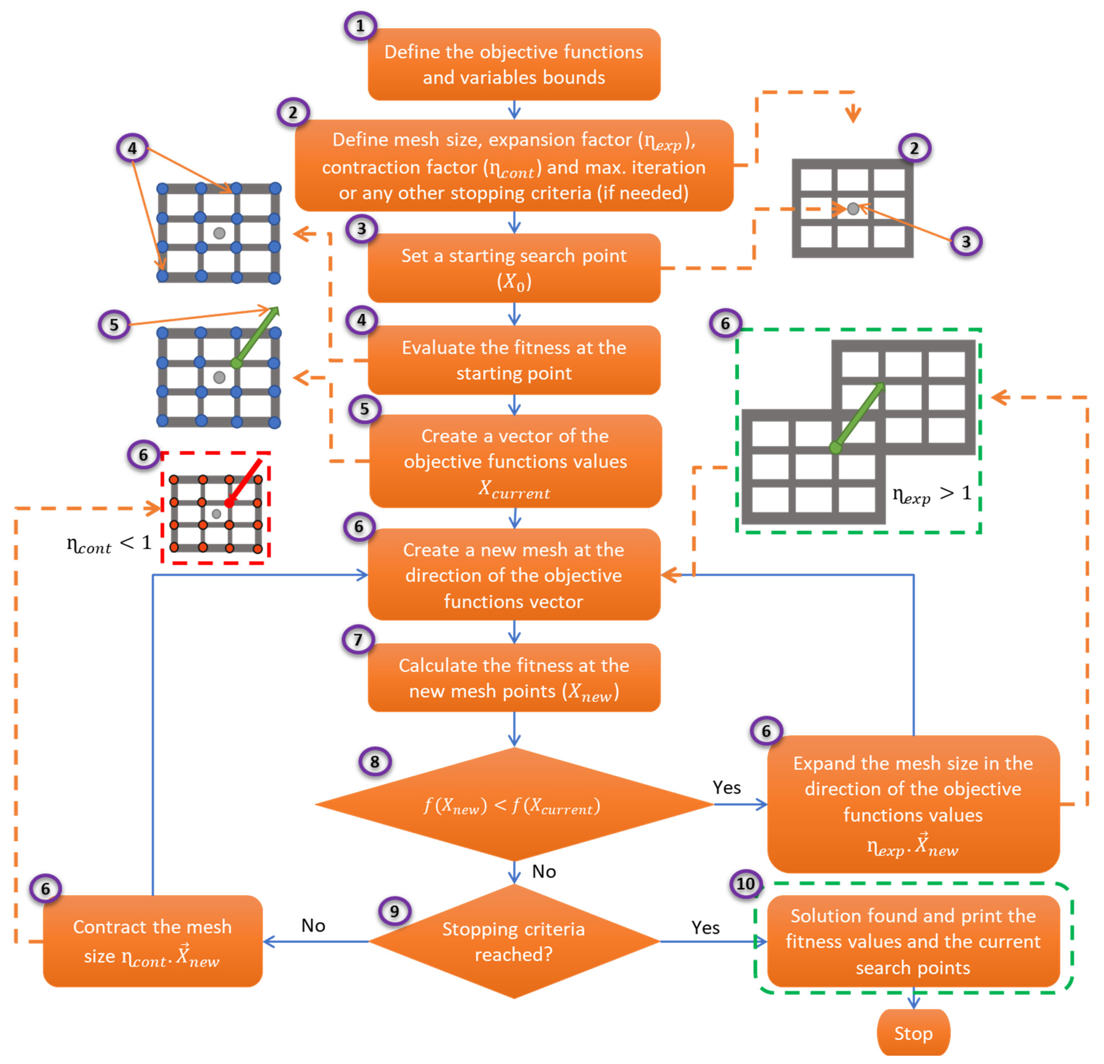
2.4. Optimization Algorithms

There are many multi-objective optimization techniques in the literature that showed robustness in finding the optimal solution through the recent decades, especially in the manufacturing field. However, the researchers introduced many novel approaches that could outperform the conventional and well-known techniques through benchmarking problems. That is, the selection of the gray wolf optimizer (GWO) and weighted value gray wolf optimizaer (WVGWO) algorithms against the robust multi-objective genetic algorithm (MOGA) and multi-objective pareto search algorithm (MOPSA) shows a great challenge between the past and the present.

Figure 6 and Figure 7 illustrate the flowcharts of the gray wolf optimizer (GWO) and weighted value gray wolf optimizer (WVGWO) algorithms clearly and sequentially, respectively. The idea of these two algorithms is simulating the hunting movement of wolves. Each wolf pack has a leader (alpha), two mid-ranking wolves (beta and delta), and the rest of the pack is called (omega). Both algorithms start with initiating a random GW population that consists of vectors of the process parameters, for example, $\overrightarrow{X_i}=[f_{r_i} v_{c_i} a_{p_i}]$ for $i=1:n$ (population size). These vectors are evaluated and sorted ascendingly. The first three vectors with best fitness function $[\begin{array}{cccc}\mathrm{M}\mathrm{R}\mathrm{R}& \mathrm{R}& \mathrm{R}\mathrm{a}& \mathrm{T}]\end{array}$ are the strongest wolves in the pack (alpha, beta, and delta). In order to find a new prey during the hunt, wolves move randomly in random directions. These directions are estimated by three parameters $(\begin{array}{ccc}a& \overrightarrow{A}& \overrightarrow{C}\end{array})$ that change their values and direction in each new iteration (t). After each movement, the fitness function is evaluated and sorted in order to find the new leaders. The difference between the aforementioned algorithms is that the new location of the whole pack is calculated by the average of the three positions of the alpha, beta, and delta wolves in GWO as in Step 8 in Figure 6 [19], and weighted average in WVGWO as in Step 10 in Figure 7 [20]. The weighted values of WVGWO are dependent on the iteration number as shown in Steps 3 and 4 in Figure 7. Finally, the new population becomes an output that is checked for reaching the maximum iteration number or convergence condition. The algorithms terminate after satisfying one of the latter two conditions.

Next, a MOGA flowchart is depicted in detail in Figure 8. The first three steps depend on generating a random population, calculating the fitness of this population, and sorting it. Each chromosome in the population is the set of the used parameters $C{h}_i=\begin{array}{ccc}\{f_{r_i}& V_{c_i}& a_{p_i}\}\end{array}$ for $i=1:n$. In Step 4 in Figure 8, the selection of the elitist chromosomes of each population occurs with a decision of keeping a certain percentage of chromosomes, performing the crossover method to another percentage of chromosomes, and mutating the rest of population. To simplify this step, an example is shown in Figure 8, as keeping best 20%, doing crossover to 60%, and mutating the rest 20%. Then the fitness of the new population is recalculated. Finally, two termination criteria are followed whether a convergence condition is achieved or reaching the maximum population generation number. If none of the latter mentioned conditions applied, the population is returned to the next generation by following the selection, crossover, and mutation steps again.

The final algorithm used in this research is the multi-objective pareto search algorithm (MOPSA) in MATLAB. The function “paretosearch” in MATLAB applies the pattern search algorithm that is illustrated in depth in Figure 9. The initial step in this algorithm is to define the objective functions and the decision variables’ bounds, in addition to the initial search point, search mesh size, and two factors of mesh expansion and contraction. The idea of this algorithm is to define a grid or mesh around a certain point, $X_0=(\begin{array}{ccc}{f}_{r_0}& V_{c_0}& a_{p_0})\end{array}$, at which the objective function fitness values are calculated and transformed into a directional vector, ${\overrightarrow{X}}_0=[\begin{array}{cccc}{\mathrm{MRR}}_0& {\mathrm{Ra}}_0& {\mathrm{R}}_0& {\mathrm{T}}_0\end{array}]$, in addition to the grid points around this point. If the mesh is a success $(fitness({\overrightarrow{X}}_{new})<fitness({\overrightarrow{X}}_{current}))$, the mesh size is expanded by factor ${\eta }_{\exp }$; if not, the mesh size is contracted by factor ${\eta }_{cont}$. In this algorithm, the stopping criterium is defined as (mesh tolerance/number of variables)² by default. Otherwise, a function tolerance can be used.

3. Results and Discussion

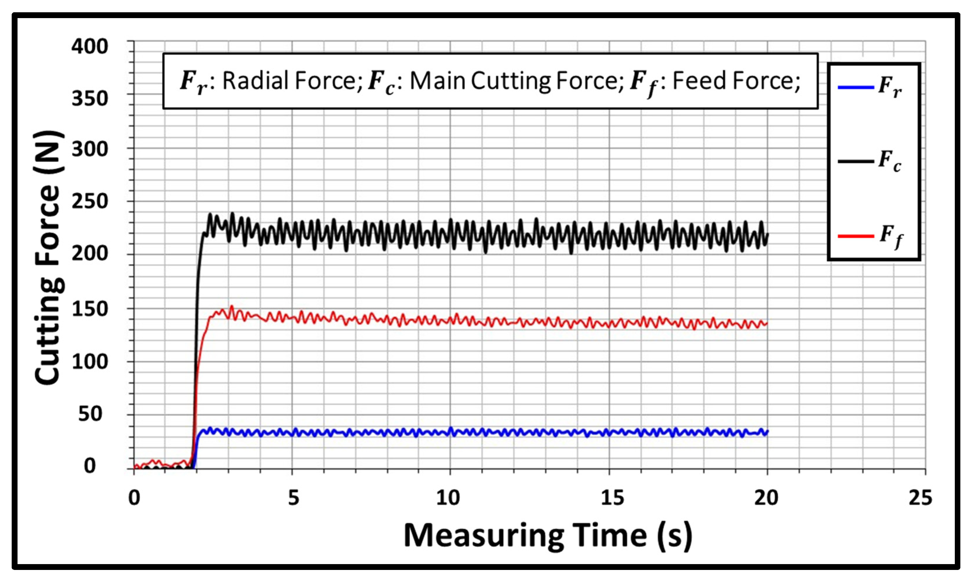
3.1. Experimental Results

Figure 10 shows the results of the turning trials conducted at a cutting speed of 80 m/min for the nine combinations of three depths of cut and three feed rates. The reported responses are the surface roughness, resultant cutting force, cutting temperature, and materials removal rate. For the three levels of depths of cut, the generated surface roughness increases with the increase in applied feed rate. Similar proportional trends to feed rates at a constant depth of cut are observed for the resultant cutting forces and temperature.

Figure 11 and Figure 12 illustrate the results of the machining tests obtained at higher cutting speeds of 120 m/min and 160 m/min under the same nine sets of feed rates and depths of cut. Again, in both figures, and similar to the results presented in Figure 10, proportional trends between the applied feed rates and obtainable surface roughness, cutting forces, and temperatures are detected. Moreover, the increase in depth of cut is found to lead to an increase in all process responses when the feed rate and cutting speeds are kept constant. When comparing the results reported in the three figures, one can see that the applied cutting speed has a negative effect wherein its higher value leads to an increase in the generated cutting force, and in the temperature and surface roughness, as well. Nevertheless, the increase in the three cutting parameters has led to an obvious increase in the cutting temperature, cutting forces, and achievable surface roughness; it also led to a significant increase in the material removal rate. This clearly indicate the trade-off between the negative and positive effect of the process parameters, and thus the need for the application of multi-objective optimization algorithms that help maximize the process productivity while keeping the other three responses, namely cutting force, cutting temperature, and surface roughness, to a minimum.

3.2. Mathematical Model Regression

The MATLAB linear quadratic regression toolbox was used. The independent variables of the model are the process parameters, feed rate ($f_r$) in mm/rev, cutting speed ($v_c$) in m/min, and depth of cut ($a_p$) in mm. In order to obtain higher accuracy, we modeled the normalized values of the independent variables in the interval by Equation (2). Hence, adding the subscript n to the variables symbols is required. That is, the modified symbols are $f_{r_n}$, $v_{c_n}$, and $a_{p_n}$.

$$x^{\backslash \backslash }=2\frac{x-x_{\min }}{x_{\max }-x_{\min }}-1$$

(2)

The obtained models of the surface roughness (Ra) with R-squared = 94.7% and p-value = 4.11 × 10⁻⁹, resultant cutting force (R) with R-squared = 89.6% and p-value = 1.04 × 10⁻⁶, and the generated cutting temperature (T) with R-squared = 75.6% and p-value = 0.000822 are shown in Equations (3)–(5), as follows:

$$\begin{array}{l}\mathrm{Ra}=1.6021+0.86533f_{r_n}+0.31078V_{c_n}+0.35672a_{p_n}\\ +0.12058f_{r_n}{V}_{c_n}+0.098417f_{r_n}{a}_{p_n}+0.15775V_{c_n}{a}_{p_n}\\ +0.24956f_{r_n}{}^2-0.015778V_{c_n}{}^2-0.38461a_{p_n}{}^2\end{array}$$

(3)

$$\begin{array}{l}\mathrm{R}=322.37+93.266f_{r_n}-9.733V_{c_n}+110.86a_{p_n}\\ -2.5992f_{r_n}{V}_{c_n}+25.431f_{r_n}{a}_{p_n}-18.812V_{c_n}{a}_{p_n}\\ +28.028f_{r_n}{}^2-38.266V_{c_n}{}^2-24.072a_{p_n}{}^2\end{array}$$

(4)

$$\begin{array}{l}\mathrm{T}=477.17+10.211f_{r_n}-0.22778V_{c_n}+3.2833a_{p_n}\\ -8.0583f_{r_n}{V}_{c_n}-4.7833f_{r_n}{a}_{p_n}-5.85V_{c_n}{a}_{p_n}\\ +1.7f_{r_n}{}^2-9.2833V_{c_n}{}^2-6.0167a_{p_n}{}^2\end{array}$$

(5)

Meanwhile, the material removal rate (MRR) is a deterministic formula, with the actual variable values by Equation (6) as follows:

$$\mathrm{MRR}=1000f_r{V}_c{a}_p$$

(6)

The average absolute errors between both the output of the experimental trials and the regression model are 15% for the surface roughness (Ra), 10.6% for the resultant cutting force (R), and 1.2% for the temperature (T). The comparison between the experimental trials and the obtained model are shown in Figure 13a–c.

3.3. Optimization Model and Results

The optimization algorithms used in this research have almost the same inputs. The objective functions and lower and upper bounds are the same for all algorithms, while the initial searching point differs from one algorithm to another. The optimization model is presented in

Table 6. Optimization model development.

Item	Description
Decision variables	$\begin{array}{ccc}{f}_r& {\nu }_c& a_p\end{array}$
Objective functions	$\begin{array}{l}\max \left(\mathrm{MRR}\right)\\ \min \left(\mathrm{Ra}\right)\\ \min \left(\mathrm{R}\right)\\ \min \left(\mathrm{T}\right)\end{array}$
Lower bounds	$\begin{array}{ccc}{f}_r& {\nu }_c& a_p\\ 0.045& 80& 0.50\end{array}$
Upper bounds	$\begin{array}{ccc}{f}_r& {\nu }_c& a_p\\ 0.135& 160& 1.00\end{array}$
Initial point	$\begin{array}{ccc}{f}_r& {\nu }_c& a_p\\ 0.045& 80& 0.50\end{array}$, otherwise, it depends on the algorithm.

. The objective functions aim to find the maximum MRR and the minimum Ra, R, and T. The model is limited to the lower and upper bounds of the experiment and the developed regression model. Hence, the optimal results are located inside these intervals.

The first two algorithms, GWO and WVGWO, were used with the same population size (100) and maximum iteration number (1000). Moreover, the initial point is created randomly. The optimal running conditions obtained by GWO are a feed rate of 0.070 mm/rev, cutting speed of 102.8 m/min, and depth of cut of 0.55 mm. These conditions give a best Ra of 0.717 µm, an MRR of 3957.8 mm³/min, an R of 181.55 N, and a T of 459.9 °C. Meanwhile, the WVGWO achieved different optimal decision variables for feed rate, cutting speed, and depth of cut as 0.05, 156.5, and 0.57, respectively. The optimal objectives fitness of WVGWO are a best MRR of 4460.25 mm³/min, Ra of 0.719 µm, R of 161 N, and T of 463.5 °C. Meanwhile, the MOGA and MOPSA algorithms used the default MATLAB values of population size and maximum iterations without changing the optimization function options. However, the initial point in both algorithms is as shown in Table 6. The optimal running conditions obtained by MOGA are a feed rate of 0.075 mm/rev, cutting speed of 91.5 m/min, and depth of cut of 0.55 mm. The corresponding optimal response of the obtained variables are MRR = 3774.37 mm³/min, Ra = 0.739 µm, R = 175.35 N, and T = 456.8 °C. Last, the MOPSA algorithm outperformed other algorithms, giving the optimal running conditions as a feed rate of 0.090 mm/rev, cutting speed of 82.3 m/min, and depth of cut of 0.50 mm. These optimal conditions reflected the objective functions, giving the best resultant cutting force of 146.8 N and best temperature of 454.9 °C, while the surface roughness is 0.721 and the material removal rate = 3703.3 mm³/min. Figure 14 shows a radar illustration of the optimal results obtained by the four algorithms.

Meanwhile, there is an optimization investigation that shows that the optimal surface quality during the dry turning of AISI 1045 can be obtained by the genetic algorithm (GA) at $v_c$ = 149 m/min, $f_r$ = 0.18 mm/rev, and $a_p$= 0.27mm. Moreover, this investigation provides a multi-decision model that is capable of selecting the optimal cutting parameters in different cooling conditions, namely dry, flood, and MQL-nano fluid, and targeting different objective outcomes, namely surface quality, power consumption, and machining cost [29]. This led to the investigation carried out in this research to develop such a model that provides the manufacturers with a guiding envelope of the turning parameters.

In order to determine which algorithm provides the best results, a minimum goal scoring method is used. This method is supposed to work by sorting the results of all algorithms in a matrix form based on each objective function. Then it assigns weights from 1 to 4 to the objective functions in a vector form ascendingly based on the preference of the objective function. This led to our suggesting three case scenarios, as shown in Figure 15. For example, Case 1 is sorting the preference of the objective functions as Ra, R, T, and MRR. Then, multiplying the Case 1 vector by the rank matrix will give a score for each algorithm. Eventually, the minimum score is the best solution.

The results of the three cases are illustrated in

Table 7. Optimal solutions comparison of different used algorithms.

Algorithm	Parameter			Best Rank				Objective Functions Priority
	${\mathit{f}}_{\mathit{r}}$	${\mathit{v}}_{\mathit{c}}$	${\mathit{a}}_{\mathit{p}}$	MRR	Ra	R	T	Case 1 (a)	Case 2 (b)	Case 3 (c)
GWO	0.07	102.8	0.55	2	1	4	3	26	27	29
WVGWO	0.05	156.5	0.57	1	2	2	4	22	25	26
MOGA	0.075	91.5	0.55	3	4	3	2	28	27	27
MOPSA	0.09	82.3	0.5	4	3	1	1	24	21	18

(a) Case 1: Ra > R > T > MRR. (b) Case 2: Ra > R > MRR > T. (c) Case 3: Ra > MRR > R > T.

. In Case 1, the optimal solution to be considered as the best optimal solution is the WVGWO solution. For Cases 2 and 3, MOPSA outperformed the other algorithms’ scores.

To evaluate the effect of the dry cutting on the dimensional tolerance compared to that of the wet conditions, three machining experiments were conducted. Cylindrical specimens of 60 mm nominal diameter and 55 mm cutting length were used. The cutting length was divided into two sections separated by a 5 mm width groove. Hence, the cutting operation experiment was run over a length of 25 mm for each type of cutting condition (wet/dry), as shown in Figure 16. The test run starts to cut the first 25 mm long section with wet condition, after which the cooling is stopped during the cut of the after-groove 25 mm section. The runs were conducted at the optimal speed, depth, and feed rate recommended by the optimization algorithm, i.e., 156.5 m/min, 0.57 mm, and 0.05 mm/rev, respectively. In addition, three other feed rates chosen around the optimal value (0.045 mm/rev, 0.056 mm/rev, and 0.070 mm/rev) were also tested, knowing the sensitivity of this parameter Each test was conducted three times with different passes (1, 2, and 3), while measuring the diameter three times along the 25 mm length for each sample. The average values of the resultant diameter are shown in

Table 8. Effect of dry and wet conditions on dimensional tolerances.

Test No.	${\mathit{v}}_{\mathit{c}}$ (m/min)	${\mathit{a}}_{\mathit{p}}$ (mm)	${\mathit{f}}_{\mathit{r}}$ (mm/rev)	Nominal Dia. (60 mm)	Dry			Wet			Error Diff.% In Dry/Wet
				Request Dia.	Actual Dia.	Diff.	%Error	Actual Dia.	Diff.	%Error
1	156.5	0.57	0.045	58.86	58.90	0.04	0.068%	58.88	0.02	0.034%	0.034%
2			0.056	57.72	57.77	0.05	0.087%	57.74	0.02	0.035%	0.052%
3			0.070	56.58	56.64	0.06	0.10%	56.61	0.03	0.053%	0.047%

. The results show a negligible effect on the dimensional accuracy of wet and dry conditions with a maximum average difference of about 0.053%. The main effect of dry conditions will be on the surface roughness and cutting forces and tool wear; however, dry conditions with steel material have a very small effect on the dimensional accuracy, unlike brass or copper. Normally, in real industrial practice, during machining, the cooling-fluid pump suddenly stops due to any reason; nevertheless, the machining process continues with minimal influence on dimensional accuracy (i.e., noisy factor). In the case that the design requirements impose a high dimensional tolerance/high quality of surface roughness (i.e., low Ra value), the grinding process is conducted after turning.

4. Conclusions and Future Work

The aim of this study was to identify cutting conditions for optimal surface quality, cutting forces and temperatures, and the productivity of turning operation of AISI 1045 alloy steel in dry condition. The process is optimized by using different multi-objective optimization algorithms: GWO, WVGWO, MOGA, and MOPSA. The outcomes of this research are listed as follows.

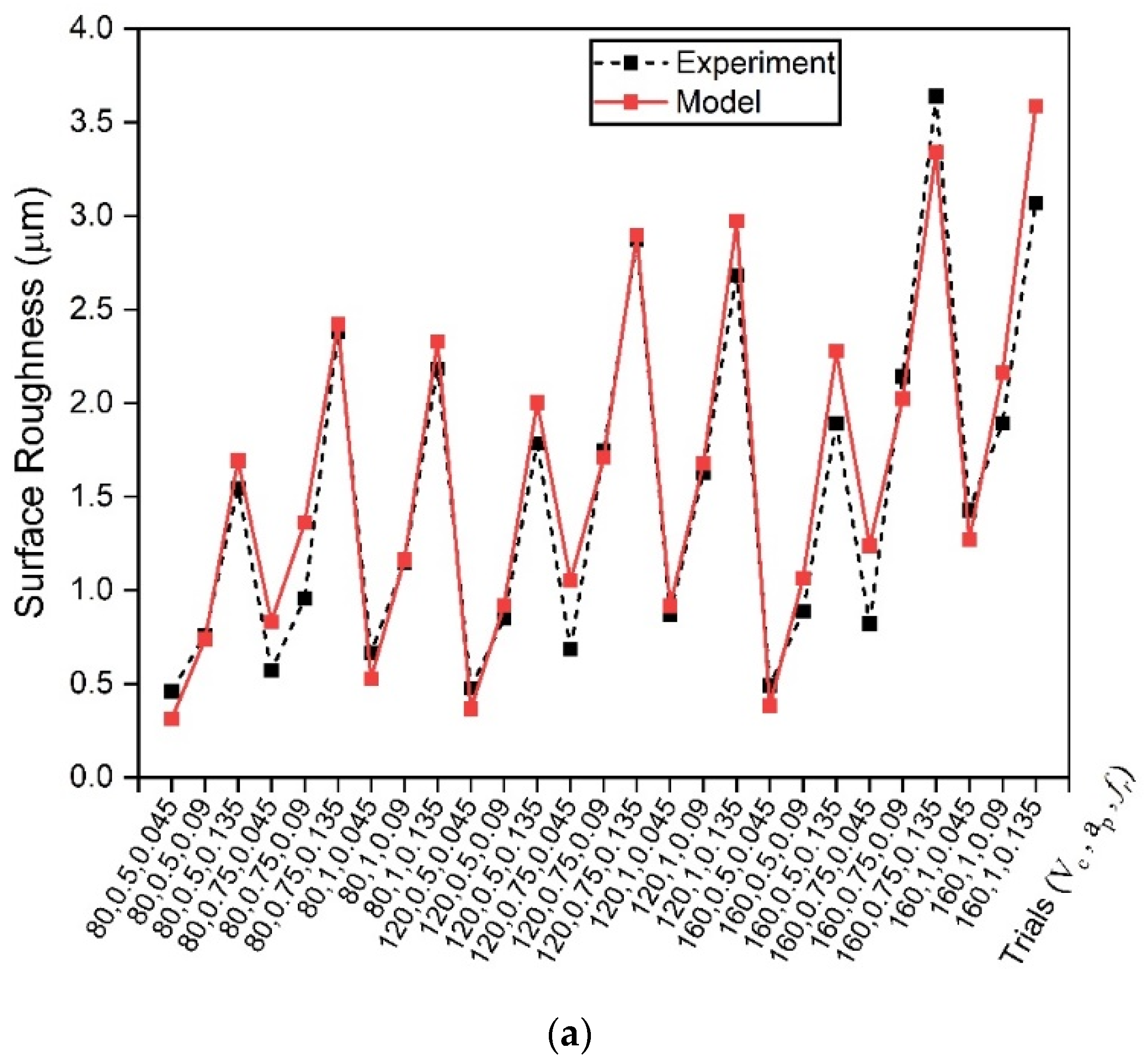
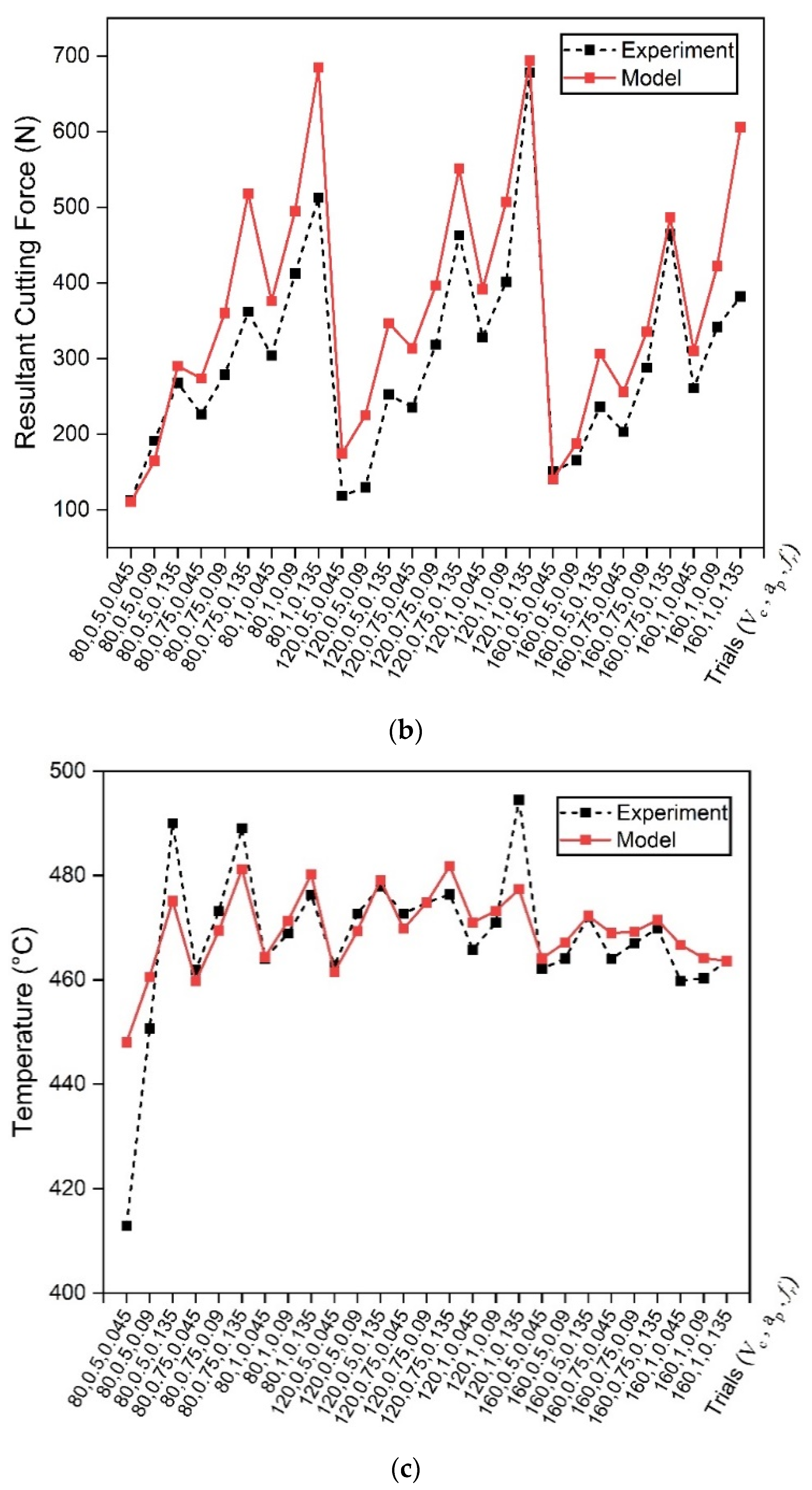
• The carried-out experiments and the developed regression mathematical model are found to be matching with average absolute errors of 15% for the surface roughness (Ra), 10.6% for the resultant cutting force (R), and 1.2% for the temperature (T). That promoted the mathematical model to represent and reflect the optimization of the real experiment.
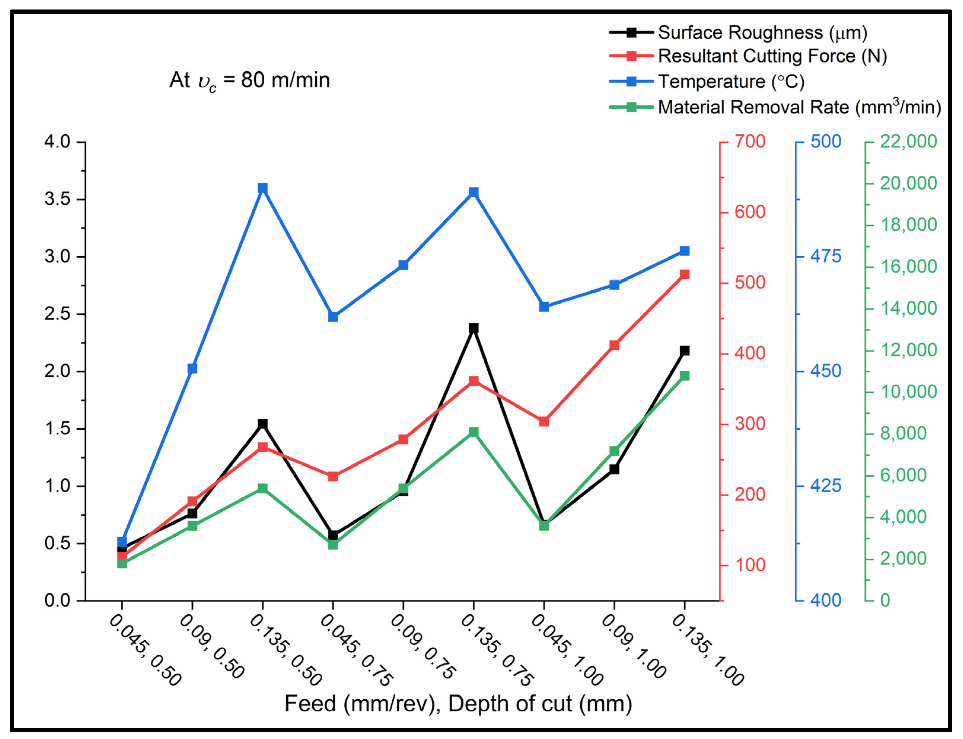
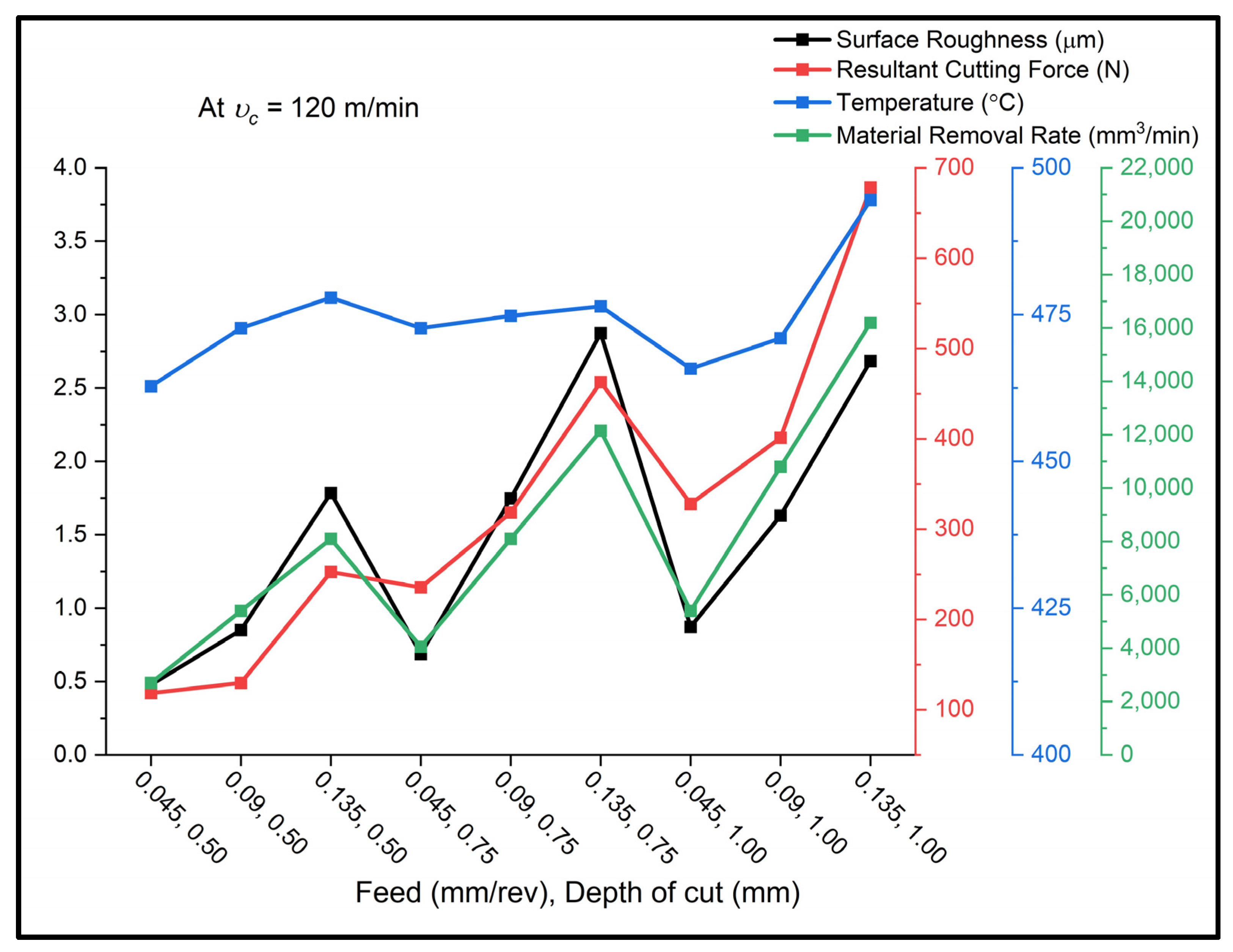
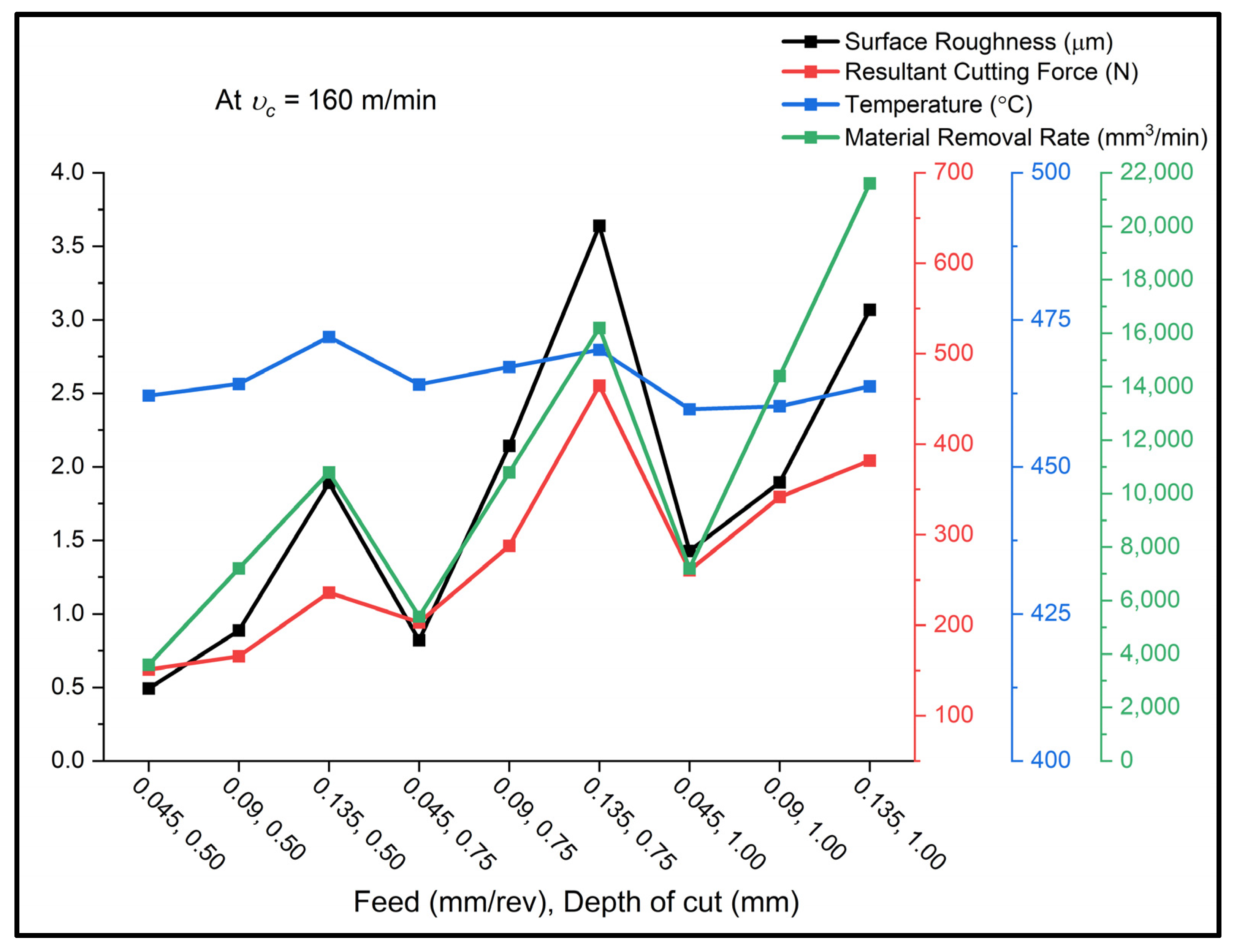
• Proportional relationships between the applied feed rates and resultant surface roughness, cutting forces, and temperatures are observed. Similar trends between depth of cut and all process responses are detected when the feed rate and cutting speeds are kept constant.
• Looking at the experimental results, it is not so difficult to conclude that the increase in the three cutting parameters has shown an obvious increase in the four cutting responses, i.e., cutting temperature, cutting forces, surface roughness, and material removal rate.
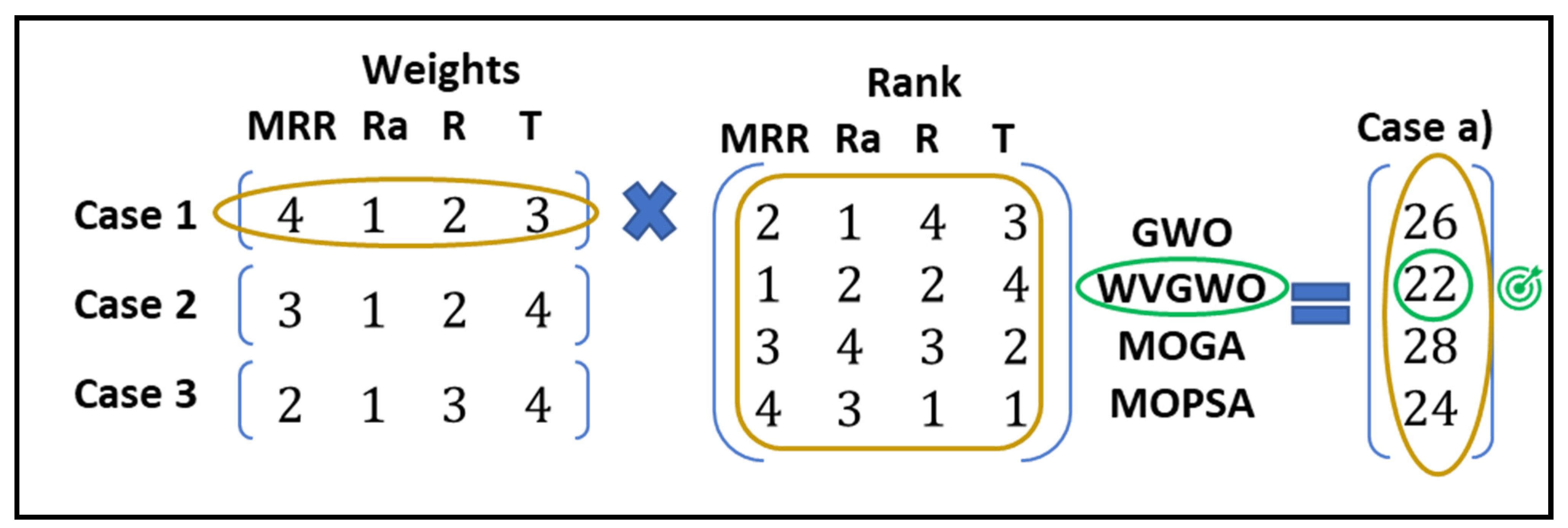
• The optimal running conditions were obtained; however, the optimal solution is dependent on the objective functions’ order.
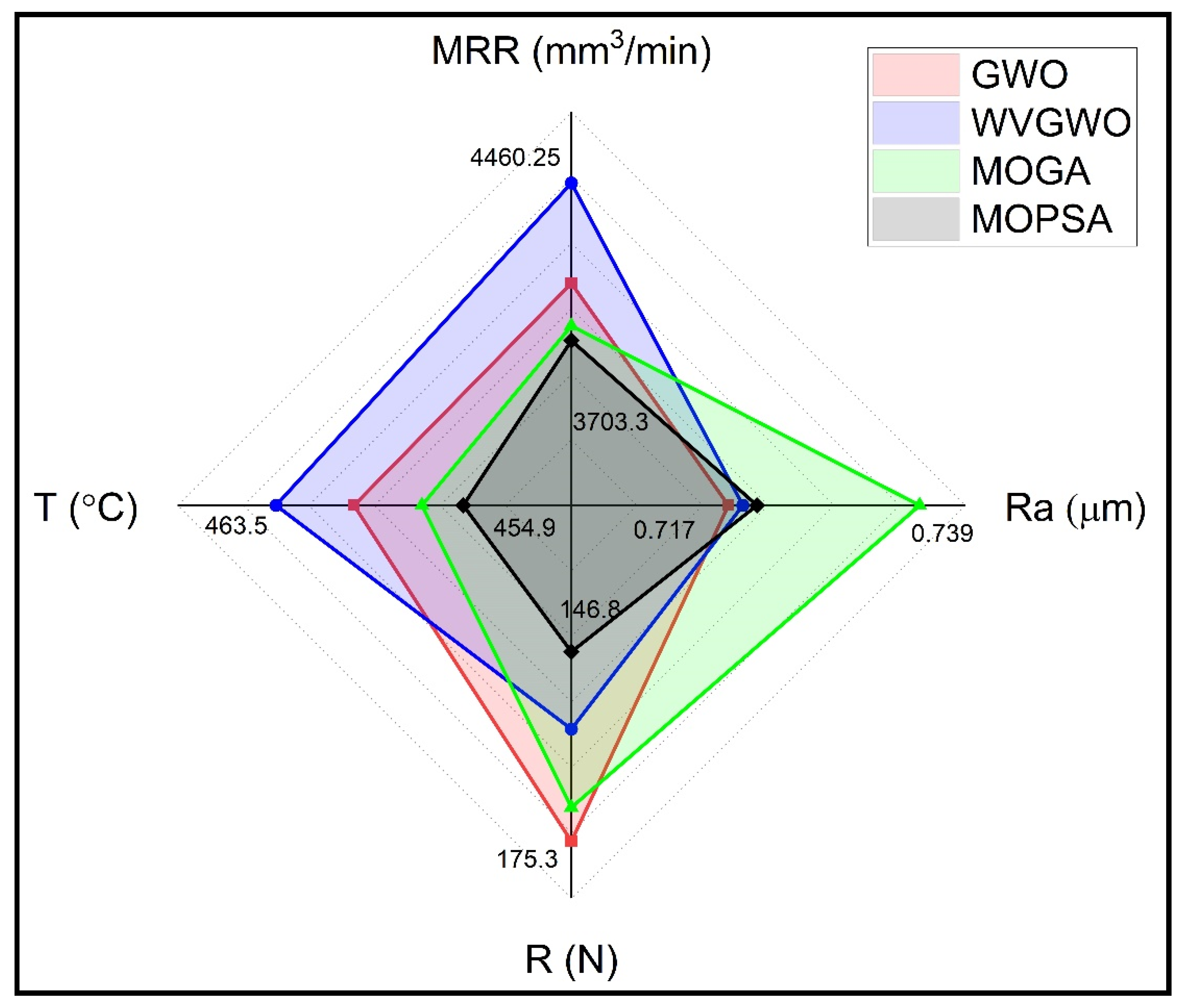
• For the most desired objective function order in Case 1, the optimal solution was obtained by the WVGWO algorithm, as the feed rate ($f_r$) is 0.05 mm/rev, the cutting speed ($v_c$) is 156.5 m/min, and the depth of cut ($a_p$) is 0.57 mm. That reflects on the objective functions and gives the best productivity (MRR = 4460.25 mm³/min), in addition to satisfying levels of surface roughness (Ra = 0.719 µm) and resultant cutting force (R = 161 N).
• In the other proposed cases, Cases 2 and 3, the MOPSA algorithm provided the optimal solution, despite of the low levels of productivity and surface quality results. The reason is that MOPSA resulted in the best resultant cutting force (R = 146.8 N) and best cutting temperature (T = 454.9 °C). The optimal running conditions are $f_r$= 0.090 mm/rev, $v_c$ = 82.3 m/min, and $a_p$ = 0.50 mm. Unfortunately, the productivity (MRR = 3703.3 mm³/min) of the MOPSA algorithm solution is 17% less than the productivity obtained by WVGWO.
• It is worth mentioning that the optimal surface quality is obtained by the GWO algorithm, as the surface roughness R is 0.717 μm. However, the optimal solution of WVGWO remains the best regardless of the surface roughness of 0.719 µm, which is 0.28% away from the best.
• The effect of cooling condition on dimensional accuracy is found to be negligible, as the dimensional error between dry and wet turning after three passes is experimentally measured as 0.053%.
• In future work, the investigation of different cutting-tool inserts geometries, such as “wiper insert”, will be carried out and compared with the current work. Moreover, the effect of running conditions and cutting-tool type on the tool life, surface roughness, and machine vibration will be studied and optimized.

References

1. Zhong, R.Y.; Xu, X.; Klotz, E.; Newman, S.T. Intelligent Manufacturing in the Context of Industry 4.0: A Review. Engineering 2017, 3, 616–630. [Google Scholar] [CrossRef]
2. Lenz, J.; MacDonald, E.; Harik, R.; Wuest, T. Optimizing smart manufacturing systems by extending the smart products paradigm to the beginning of life. J. Manuf. Syst. 2020, 57, 274–286. [Google Scholar] [CrossRef]
3. Sarker, I.H. AI-Based Modeling: Techniques, Applications and Research Issues Towards Automation, Intelligent and Smart Systems. SN COMPUT. SCI. 2022, 3, 158. [Google Scholar] [CrossRef] [PubMed]
4. Chen, X.; Li, C.; Tang, Y.; Li, L.; Li, H. Energy efficient cutting parameter optimization. Front. Mech. Eng. 2021, 16, 221–248. [Google Scholar] [CrossRef]
5. Abbas, A.T.; Al-Abduljabbar, A.A.; Alnaser, I.A.; Aly, M.F.; Abdelgaliel, I.H.; Elkaseer, A. A Closer Look at Precision Hard Turning of AISI4340: Multi-Objective Optimization for Simultaneous Low Surface Roughness and High Productivity. Materials 2022, 15, 2106. [Google Scholar] [CrossRef]
6. Qehaja, N.; Jakupi, K.; Bunjaku, A.; Bruçi, M.; Osmani, H. Effect of Machining Parameters and Machining Time on Surface Roughness in Dry Turning Process. Procedia Eng. 2015, 100, 135–140. [Google Scholar] [CrossRef]
7. Suhail, A.H.; Ismail, N.; Wong, S.V.; Jali, N.A.A. Workpiece Surface Temperature for In-process Surface Roughness Prediction using Response Surface Methodology. J. Appl. Sci. 2011, 11, 308–315. [Google Scholar] [CrossRef] [Green Version]
8. Kuntoğlu, M.; Aslan, A.; Pimenov, D.Y.; Giasin, K.; Mikolajczyk, T.; Sharma, S. Modeling of Cutting Parameters and Tool Geometry for Multi-Criteria Optimization of Surface Roughness and Vibration via Response Surface Methodology in Turning of AISI 5140 Steel. Materials 2020, 13, 4242. [Google Scholar] [CrossRef]
9. Fnides, B. Cutting forces and surface roughness in hard turning of hot work steel X38CrMoV5-1 using mixed ceramic. Mechanics 2008, 70, 73–78. [Google Scholar]
10. Rabu, A.R. Correlation Among The Cutting Parameters, Surface Roughness And Cutting Forces In Turning Process By Experimental Studies. In Proceedings of the Design and Research Conference, Assam, India, 12–14 December 2014; IIT Guwahati: Assam, India, 2014. [Google Scholar]
11. Hernández-González, L.W.; Curra-Sosa, D.A.; Pérez-Rodríguez, R.; Zambrano-Robledo, P.D.C. Modeling Cutting Forces in High-Speed Turning using Artificial Neural Networks. TecnoLógicas 2021, 24, e1671. [Google Scholar] [CrossRef]
12. Kamruzzaman, M.; Dhar, N.R. Effect of High-Pressure Coolant on Temperature, Chip, Force, Tool Wear, Tool Life and Surface Roughness in Turning AISI 1060 Steel. Gazi Univ. J. Sci. 2009, 22, 359–370. [Google Scholar]
13. Kuntoğlu, M.; Gupta, M.K.; Aslan, A.; Salur, E.; Garcia-Collado, A. Influence of tool hardness on tool wear, surface roughness and acoustic emissions during turning of AISI 1050. Surf. Topogr. Metrol. Prop. 2022, 10, 015016. [Google Scholar] [CrossRef]
14. Abdallah, F.; Abdelwahab, S.A.; Aly, W.I.A.; Ahmed, I. Influence of Cutting Factors on the Cutting Tool Temperature and Surface Roughness of Steel C45 during Turning Process. IJRT 2019, 6, 8. [Google Scholar]
15. Patil, S.; Jadhav, S.; Kekade, S.; Supare, A.; Powar, A.; Singh, R.K.P. The Influence of Cutting Heat on the Surface Integrity during Machining of Titanium Alloy Ti6Al4V. Procedia Manuf. 2016, 5, 857–869. [Google Scholar] [CrossRef] [Green Version]
16. He, G.; Liu, X.; Yan, F. Research on the dynamic mechanical characteristics and turning tool life under the conditions of excessively heavy-duty turning. Front. Mech. Eng. 2012, 7, 329–334. [Google Scholar] [CrossRef]
17. Abbas, A.T.; Abubakr, M.; Elkaseer, A.; Rayes, M.M.E.; Mohammed, M.L.; Hegab, H. Towards an Adaptive Design of Quality, Productivity and Economic Aspects When Machining AISI 4340 Steel With Wiper Inserts. IEEE Access 2020, 8, 159206–159219. [Google Scholar] [CrossRef]
18. Jia, S.; Wang, S.; Lv, J.; Cai, W.; Zhang, N.; Zhang, Z.; Bai, S. Multi-Objective Optimization of CNC Turning Process Parameters Considering Transient-Steady State Energy Consumption. Sustainability 2021, 13, 13803. [Google Scholar] [CrossRef]
19. Mirjalili, S.; Saremi, S.; Mirjalili, S.M.; Coelho, L.d.S. Multi-objective grey wolf optimizer: A novel algorithm for multi-criterion optimization. Expert Syst. Appl. 2016, 47, 106–119. [Google Scholar] [CrossRef]
20. Gao, Z.-M.; Zhao, J. An Improved Grey Wolf Optimization Algorithm with Variable Weights. Comput. Intell. Neurosci. 2019, 2019, 1–13. [Google Scholar] [CrossRef]
21. Do, T.-V.; Nguyen, Q.-M. Optimizing Machining Parameters to Minimize Surface Roughness in Hard Turning SKD61 Steel Using Taguchi Method. J. Mech. Eng. Res. Dev. 2021, 44, 214–218. [Google Scholar]
22. Sarıkaya, M.; Güllü, A. Taguchi design and response surface methodology based analysis of machining parameters in CNC turning under MQL. J. Clean. Prod. 2014, 65, 604–616. [Google Scholar] [CrossRef]
23. Kuntoğlu, M.; Sağlam, H. Investigation of progressive tool wear for determining of optimized machining parameters in turning. Measurement 2019, 140, 427–436. [Google Scholar] [CrossRef]
24. Ribeiro, J.E.; César, M.B.; Lopes, H. Optimization of machining parameters to improve the surface quality. Procedia Struct. Integr. 2017, 5, 355–362. [Google Scholar] [CrossRef]
25. Al-Shayea, A.; Abdullah, F.M.; Noman, M.A.; Kaid, H.; Nasr, E.A. Studying and Optimizing the Effect of Process Parameters on Machining Vibration in Turning Process of AISI 1040 Steel. Adv. Mater. Sci. Eng. 2020, 2020, 1–15. [Google Scholar] [CrossRef]
26. Kuntoğlu, M.; Acar, O.; Gupta, M.K.; Sağlam, H.; Sarikaya, M.; Giasin, K.; Pimenov, D.Y. Parametric Optimization for Cutting Forces and Material Removal Rate in the Turning of AISI 5140. Machines 2021, 9, 90. [Google Scholar] [CrossRef]
27. Sidhu, A.S.; Singh, S.; Kumar, R.; Pimenov, D.Y.; Giasin, K. Prioritizing Energy-Intensive Machining Operations and Gauging the Influence of Electric Parameters: An Industrial Case Study. Energies 2021, 14, 4761. [Google Scholar] [CrossRef]
28. Dubey, V.; Sharma, A.K.; Vats, P.; Pimenov, D.Y.; Giasin, K.; Chuchala, D. Study of a Multicriterion Decision-Making Approach to the MQL Turning of AISI 304 Steel Using Hybrid Nanocutting Fluid. Materials 2021, 14, 7207. [Google Scholar] [CrossRef]
29. Abbas, A.T.; Benyahia, F.; El Rayes, M.M.; Pruncu, C.; Taha, M.A.; Hegab, H. Towards Optimization of Machining Performance and Sustainability Aspects when Turning AISI 1045 Steel under Different Cooling and Lubrication Strategies. Materials 2019, 12, 3023. [Google Scholar] [CrossRef]
Figure 1. Microstructure of AISI 1045.
Metals 13 00096 g001
Figure 2. Test rig for machining the test pieces, evaluating the cutting forces, and measuring the cutting temperature.
Metals 13 00096 g002
Figure 3. Cutting forces monitoring by Kistler 5070 at v c = 160 m/min, a p = 1 mm, and f r = 0.045 mm/rev.
Metals 13 00096 g003
Figure 4. Temperature monitoring by ThermoPro-TP8 at v c = 80 m/min, a p = 0.5 mm, and f r = 0.045 mm/rev. (a) The temperature contour view by the thermo camera. (b) The real cutting views.
Metals 13 00096 g004
Figure 5. (a) Measuring setting parameters, (b) Test rig for measuring surface roughness.
Metals 13 00096 g005
Figure 6. Flowchart of GWO algorithm.
Metals 13 00096 g006
Figure 7. Flowchart of WVGWO algorithm.
Metals 13 00096 g007
Figure 8. Flowchart of MOGA algorithm.
Metals 13 00096 g008
Figure 9. Flowchart of MOPSA algorithm.
Metals 13 00096 g009
Figure 10. The experimental results at cutting speed = 80 m/min.
Metals 13 00096 g010
Figure 11. The experimental results at cutting speed = 120 m/min.
Metals 13 00096 g011
Figure 12. The experimental results at cutting speed = 160 m/min.
Metals 13 00096 g012
Figure 13. The comparison between experiment and model results, (a) surface roughness (Ra), (b) resultant cutting force (R), and (c) temperature (T).
Metals 13 00096 g013aMetals 13 00096 g013b
Figure 14. Comparison between the optimal results obtained by the four different algorithms used.
Metals 13 00096 g014
Figure 15. Suggested minimum goal scoring method.
Metals 13 00096 g015
Figure 16. Validation of dimensional accuracy of test specimen’s dimensions.
Metals 13 00096 g016