Fast Checking of Drift Demand in Multi-Storey Buildings with Asymmetry


1
Department of Infrastructure Engineering, The University of Melbourne, Parkville, VIC 3010, Australia
2
Bushfire and Natural Hazards Cooperative Research Centre, Melbourne, VIC 3002, Australia
3
Faculty of Engineering, Computing and Science, Swinburne University of Technology, Kuching, Sarawak 93350, Malaysia
*
Author to whom correspondence should be addressed.
Buildings 2021, 11(1), 13; https://0-doi-org.brum.beds.ac.uk/10.3390/buildings11010013
Submission received: 25 November 2020
/
Revised: 22 December 2020
/
Accepted: 23 December 2020
/
Published: 28 December 2020
(This article belongs to the Section Building Structures)
Abstract
:Buildings possessing an asymmetrical arrangement of structural elements are torsionally unbalanced and can be vulnerable in a seismic event. Building codes of practices typically recommend the use of three-dimensional dynamic analysis to determine the seismic demands of a multi-storey building. Whilst most design practices are well equipped with commercial software for undertaking such analyses, designers often find it difficult to verify results. Much of the published technical articles present findings for buildings based on an idealised single-storey model. As a result of challenges in dealing with real multi-storey buildings, there has been very limited uptake of research findings in design practices. This article presents a three-tiered approach of estimating the displacement behaviour of the building in term of 3D/2D displacement ratio. The estimate can be used for verifying results reported from a computer package conveniently. The quick method provides predictions of the 3D/2D ratio and only requires the gross plan dimensions of the building to be known. The refined method requires knowledge of the torsional stiffness properties to be known, whereas the detailed method requires the eccentricity properties to be known as well. The proposed methodology is robust and reliable, as is demonstrated by case studies undertaken on six real multi-storey buildings.
1. Introduction
Reinforced concrete multi-storey buildings make up the bulk of the building stock in the world. These buildings are typically braced laterally by cantilever shear walls or core walls, which are asymmetrically disposed around the building resulting in a significant offset of the centre of rigidity (CR) from the centre of mass (CM) of the building. The offset, which is also known as the eccentricity, can result in significant displacement amplification of the building in seismic conditions, thereby increasing the vulnerability of the building to sustaining severe damage [1,2,3,4]. The displacement demand of the building is always most critical at its edges. Parameters that are particularly relevant to the seismic response behaviour are namely the elastic radius, eccentricity, radius of gyration of its mass, the natural period of vibration, and disposition of the structural elements that are close to the edges [4,5,6,7].
Some 600–700 articles have been published on the topic of torsional behaviour of asymmetrical buildings in the past three decades as reported in a comprehensive literature review [6]. Many earlier investigations based on linear elastic analyses were aimed to develop a quasi-static analysis approach to simulate dynamic torsional behaviour of asymmetrical buildings [8,9,10,11,12]. More recent studies based on non-linear analyses focussed on evaluating existing approaches recommended by design provisions and published literature in predicting the torsional behaviour of asymmetrical buildings [13,14,15,16,17,18]. The major shortcoming of analytical investigations reported in the literature was the idealisation of the building into a single-storey floor model. Given that the stiffness and eccentricity properties of the building may vary up its height and vary from floor to floor, it may not be feasible to make use of a single-storey building model to characterise the potential torsional response behaviour of a multi-storey building. For example, the unique position of the CR of the building may not be easy to identify, unlike a single storey building.
Seismic design standards [19,20,21] typically recommend the use of three-dimensional (3D) dynamic analysis for modelling the complex torsional behaviour of the building. A 3D dynamic analysis is resource-intensive and requires plenty of experience and a depth of expertise. It would be difficult for a designer to undertake a detailed evaluation of the dynamic analysis of the building as reported by a commercial package, or to undertake an independent analysis. It is recommended that the structural designer make use of a simplified method of assessment that gives predictions of the maximum displacement demand of the building expressed in the form of a 3D/2D displacement ratio (Δ3D/Δ2D) for verifying results that are reported by the commercial package. The Δ2D is the pure translational displacement (no rotation) of the building determined from the 2D model of the building with the torsional rotation of all the floors restrained. Similarly, the Δ3D is the total displacement (sum of translational and rotational deflection) of the building determined through the analysis of a 3D model of the building with the torsional restraint being released.
The authors have developed a simplified method referred to as Generalised Force Method (GFM) of analysis based on static analysis to provide estimates of the maximum displacement of multi-storey buildings. The method has been developed for low- to medium-rise buildings [5] and has been extended to the analysis of high-rise buildings incorporating higher mode effects [22] and asymmetrical buildings with bi-axial asymmetry [4]. The simplified approach of assessment as introduced herein is an extension of what is known as the Generalised Force Method (GFM), which involves the use of simple expressions for predicting the 3D/2D displacement ratio for a rectangular asymmetrical multi-storey building [1,5,22]. In this paper, the equations have been developed further to handle irregularly shaped buildings. The assessment method is facilitated further by the use of charts and simple algebraic expressions. It has been found by the authors that the amount of torsional amplification in a building possessing bi-axial asymmetry is less critical than that of a building possessing uni-axial asymmetry when all parameters are kept the same [4]. Thus, the analytical method proposed herein is based on the conditions of uni-axial asymmetry.
The multi-tiered approach of assessment, as introduced in this article, offers the option of conducting a quick, refined, or detailed assessment of the displacement demand of the building. In some cases, the quick assessment method alone suffices when the predicted displacement demands are well within the thresholds for causing damage or when the predictions are already close enough to that reported by the commercial package. The designer has the option of following through with a refined, and/or a detailed, method of assessment should more accurate assessments be warranted.
The reliability of the presented assessment methodology has been evaluated through the case study of six real buildings (of L-shape, Y-shape, U or C shape, and cross-shape on the plan). A distinguishing feature of this study is the use of real buildings to provide support for the method of assessment as opposed to using idealised (single-storey) models.
2. Procedure for Determining Torsional Amplification (Edge Displacement Ratio)
In this study, a multi-tiered approach involving a quick, refined and detailed method of assessment of the torsional amplification behaviour of a building (expressed in terms of the edge displacement ratio) is proposed. Each of the tiered methods of assessment is distinctive to each other based on the simplicity and demand on the details of the torsional parameters required to determine the edge displacement ratio. The details of the proposed method are presented in this section.
2.1. Parameters Used for Determining the Edge Displacement Ratio
Four major torsional parameters of the building are considered in this study to estimate the edge displacement ratio of the regular and irregular shaped buildings. These four parameters are the normalised distance between the edge element of the buildings and buildings’ CM (Br), the fundamental period (Tn1), the elastic radius ratio (br), and the normalised eccentricity (er). These parameters are described in the following sections.
2.1.1. Normalised Distance between the Edge Element of the Building and Its Centre of Mass
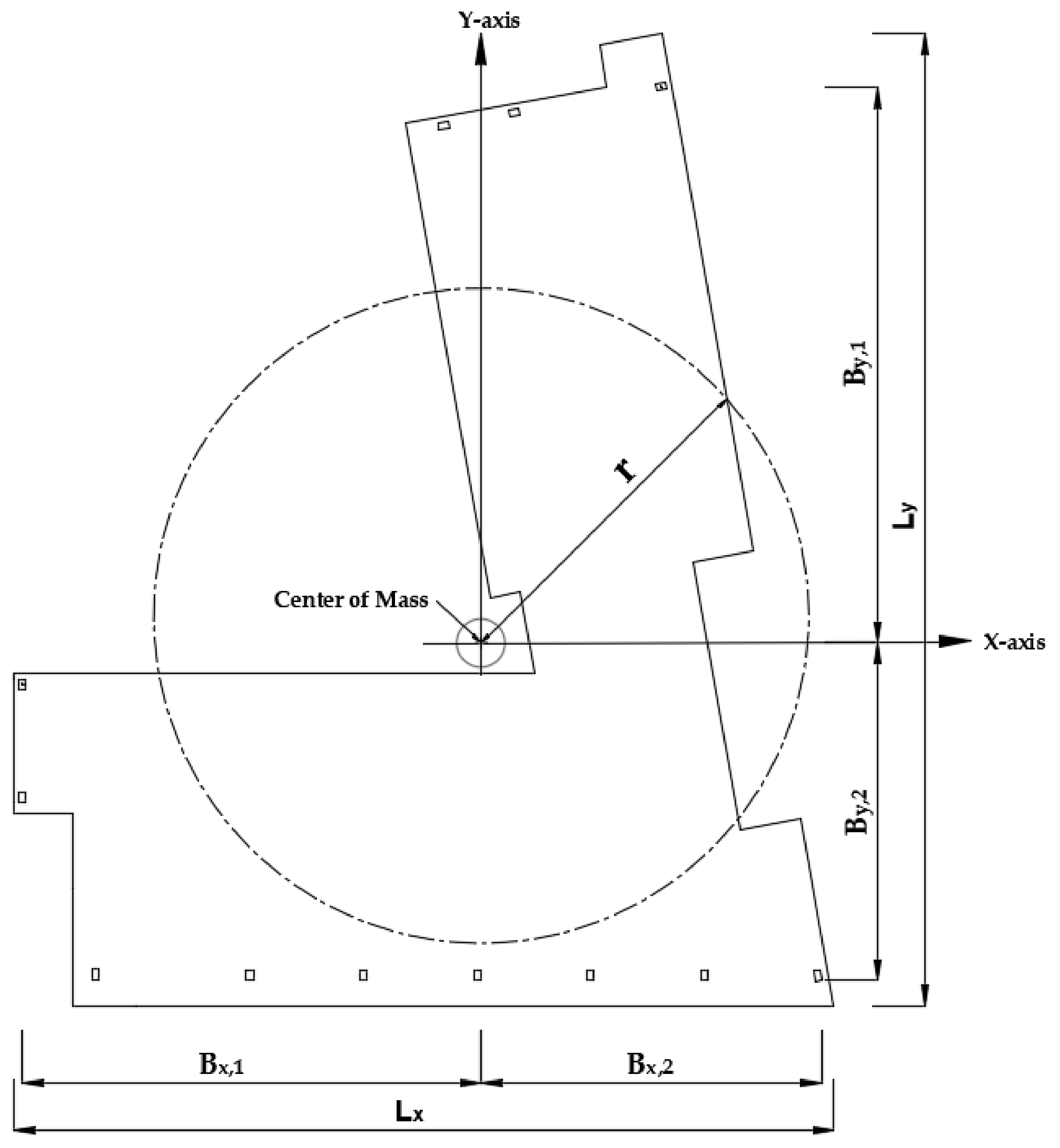
The normalised distance between the edge of the building and its centre of mass (Br) is defined as the furthest distance of the edge element (a column, frame, or wall) measured from the CM in the direction perpendicular to the direction of ground motion and normalised with respect to the mass radius of gyration (r) of the building (about the vertical axis of the floor plan). For a square or rectangular building having uniform floor mass and structural elements at the two edges, Br can be determined by normalising half of the width or length of the building to the mass radius of gyration. For a building with an irregular floor plan as shown in Figure 1, Br for the building can be expressed in term of Brx,1, Brx,2, Bry,1 and Bry,2.
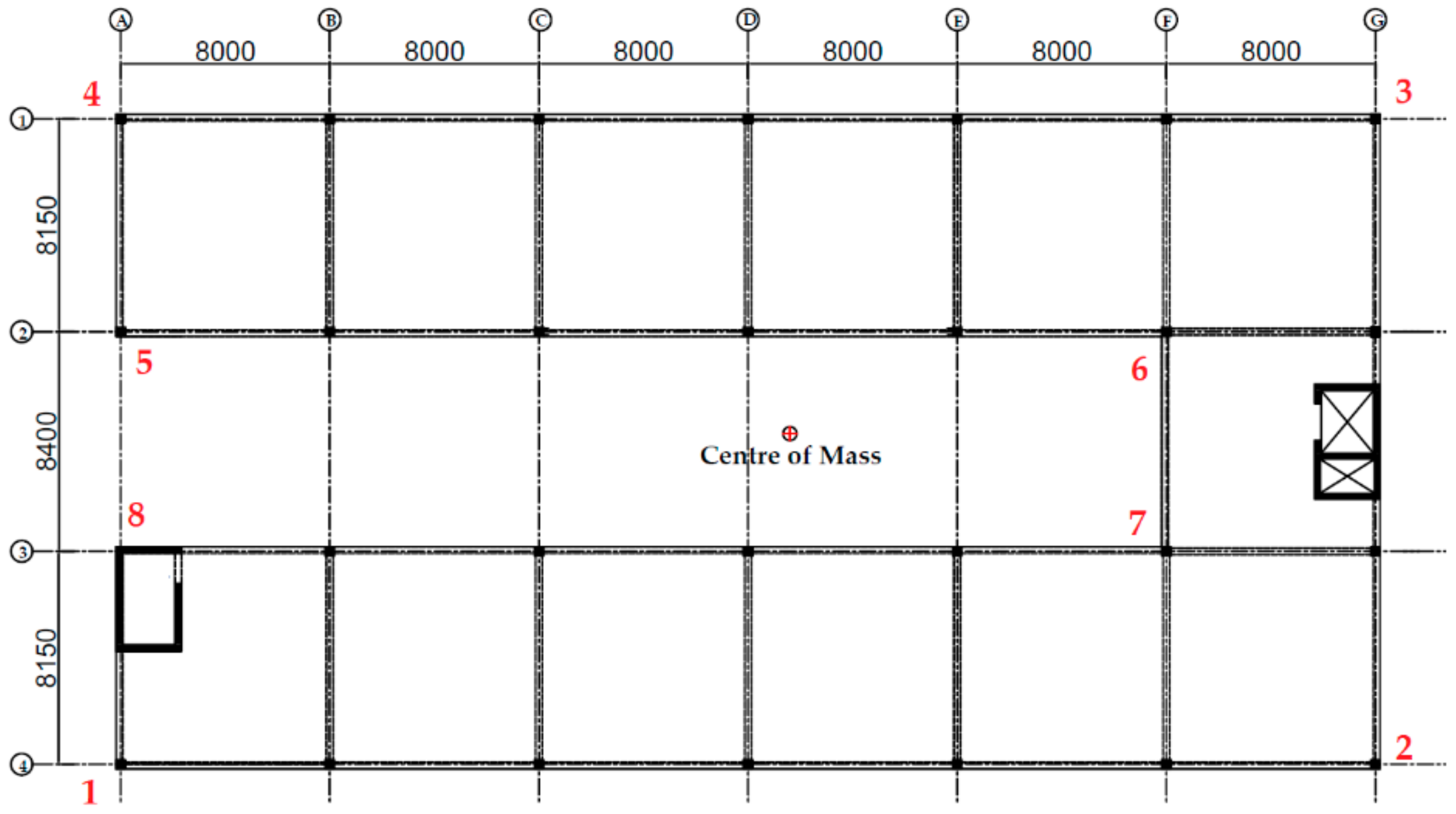
Parameter “r” is defined as the radial distance from the CM of the building about which the moment of inertia of the lumped mass of the building is equal to the moment of inertia of the actual distribution of the mass of the building. Considering a uniform mass density of the building floor, the value of “r” is expressed as the square root of the polar moment of inertia divided by the area of the building plan. For rectangular and square buildings, the value of “r” can be determined using Equation (1). For irregular buildings, the value of “r” can be determined based on manual calculations using the coordinate method given in [23] or using a computer drawing software such as AutoCAD. The coordinate method is summarised in Appendix A.1. An example calculation to determine the value of “r” for one of the case study buildings (CSB 5) is shown in Appendix A.2. The calculated value of “r” for CSB 5 was compared with that obtained using the AutoCAD software (Version 20.1, AutoDesk) and the MASSPROP command [24]. As both of these two methods gave the same value of “r”, AutoCAD was used for the other case study buildings.
where Lx and Ly are the lengths of the building about its principal directions x and y, respectively.
2.1.2. Effective Fundamental Natural Period of Vibration (Tn1) of the Building
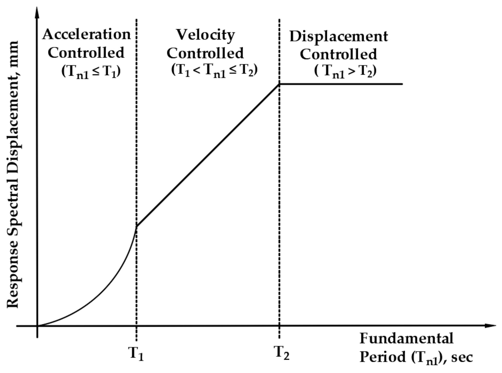
The seismic response behaviour of an asymmetrical building is controlled by either the acceleration, velocity, or displacement demand of the earthquake based on the effective fundamental natural period (Tn1) of the two-dimensional (2D) model of the building, as illustrated in Figure 2. When the value of Tn1 is less than or equal to the first corner period (T1) of the response spectrum, the seismic response behaviour of the building is considered to be “acceleration-controlled”. The building with a fundamental period greater than T1 and less than or equal to the second corner period (T2) is considered to be “velocity-controlled”. A building with a fundamental natural period exceeding T2 is considered to be “displacement-controlled”.
The effective fundamental period of the equivalent 2D building can be calculated using Equation (2) given in [3].
where
- n is the number of storeys in a building,
- mi is the mass of storey i,
- δi is the two-dimensional (2D) static deflection of the storey i of the building determined by applying horizontal equivalent static design forces at each storey i,
- Vb is the total base shear calculated as per the relevant seismic code.
2.1.3. Locating the CR and Determining the Eccentricity Parameter er
An essential step in the procedure is to locate the CR of the building by conducting static analyses. There are three methods to choose from, as outlined below. Although a building that has a rectangular shaped plan is used for illustration, the procedure is equally applicable to building plans that are irregularly shaped.
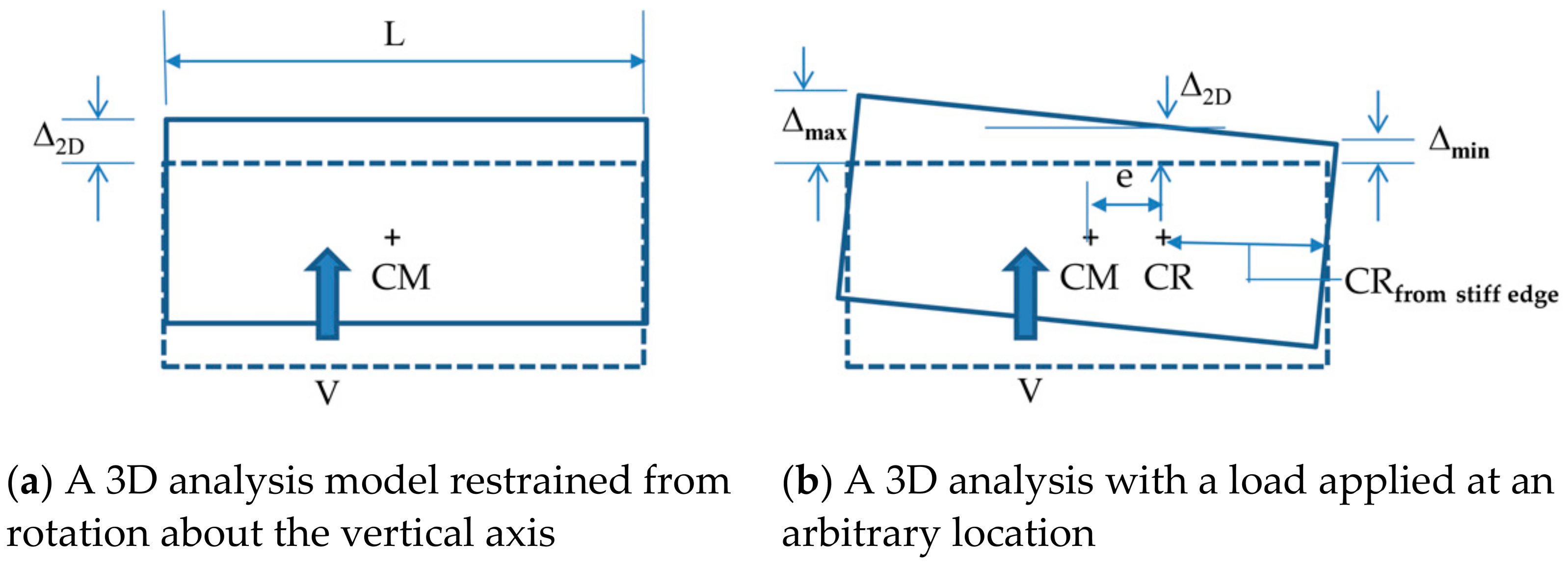
Method (1)–Apply a lateral load (V) to the 2D model of the building at an arbitrary location with the torsional rotation of all the floors restrained. The displacement of the building is accordingly denoted as Δ2D. Repeat the same analysis on a 3D model of the building with the torsional restraint being released and with the same load applied, as shown in Figure 3. The edge displacements are denoted as Δmax and Δmin. The location of the CR can be found using Equation (3).
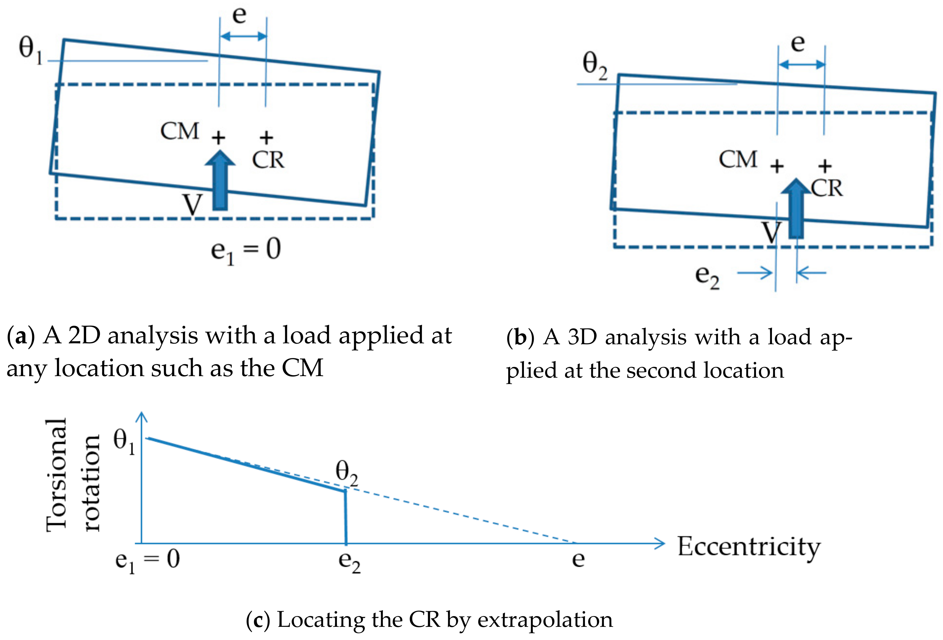
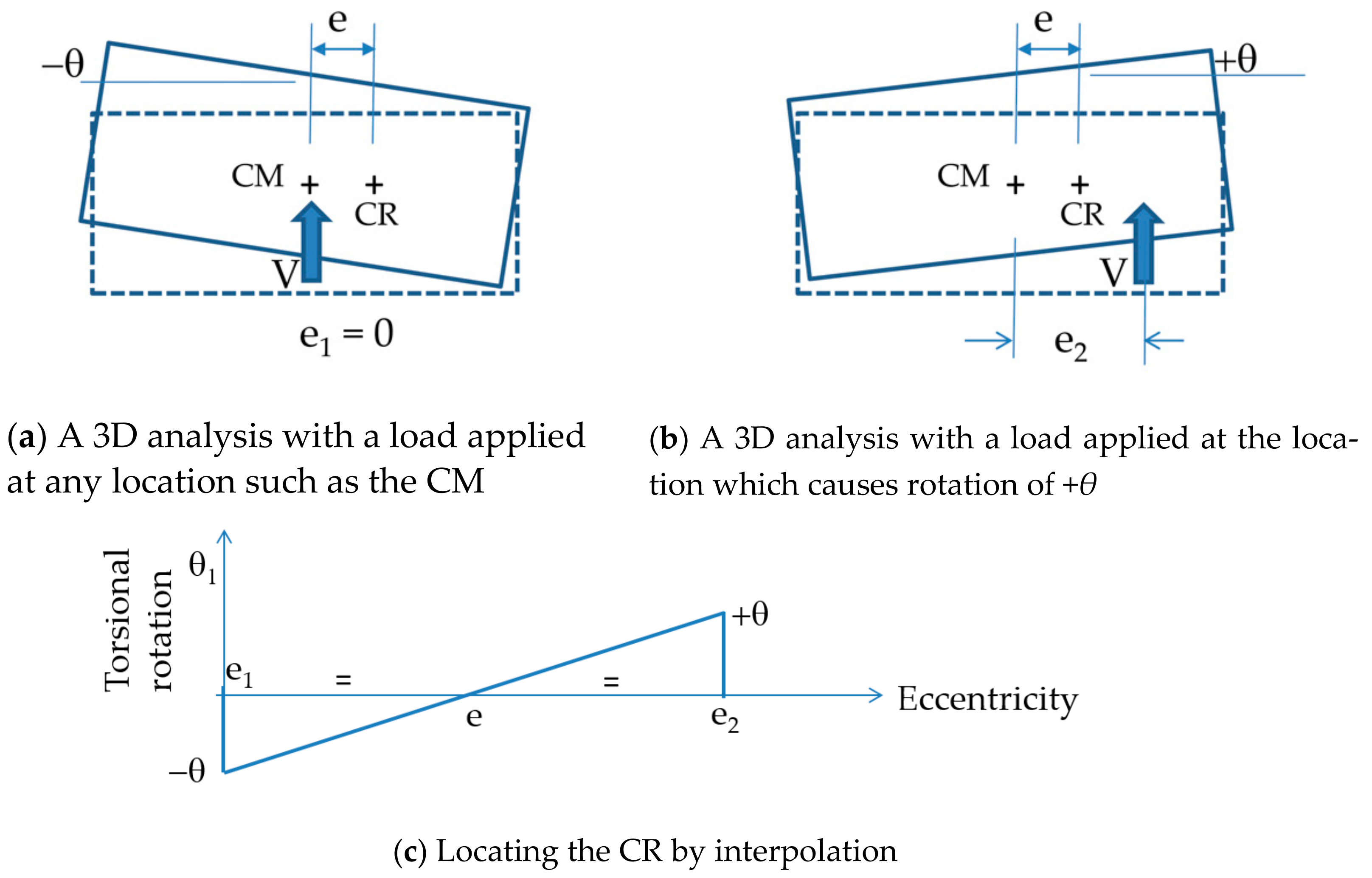
Method (2)–Apply a lateral load (V) to the 3D model of the building at two arbitrary locations in two separate load cases. Take note of the respective torsional rotations θ1 and θ2. The location of the CR can be found by extrapolation to determine the offset at which there are zero rotation results, as shown in Figure 4. The amount of displacement at the CR is equal to Δ2D. Thus, once the location of the CR is known, the value of Δ2D can be determined by scaling the edge displacement values.
Method (3)–Apply a lateral load (V) to the 3D model of the building at two locations in two separate load cases to result in rotations −θ and +θ (a few trials may be required to achieve this equality). The CR is located at the mid-point between the two load locations, as shown in Figure 5. The value of Δ2D can also be determined by scaling the edge displacement values as for Method (2).
In the foregoing illustrations, the displacements of a multi-storey building were represented by single (effective) displacement values, namely Δ2D, Δmax, and Δmin. The relationships for obtaining these parameters for given floor displacements are defined by Equations (4)–(6).
where
- n is the number of storeys of the building,
- mi is the mass of storey i,
- δmax,i, δmin,i, and δ2D,i are the minimum, maximum, and 2D static displacement of the storey i determined from computer software by applying horizontal equivalent static design forces at each storey i following the procedure given in the relevant seismic code.
The normalised eccentricity (er) is eccentricity (e) normalised with respect to the mass radius of gyration (r). Eccentricity (e) is the distance between the CM and CR of the building. The distance between the stiff edge and the CM of the building (B) is as defined in Figure 1. Refer to Equations (7) and (8) for the mathematical expressions for defining the eccentricity parameters.
2.1.4. Determining Elastic Radius Ratio br
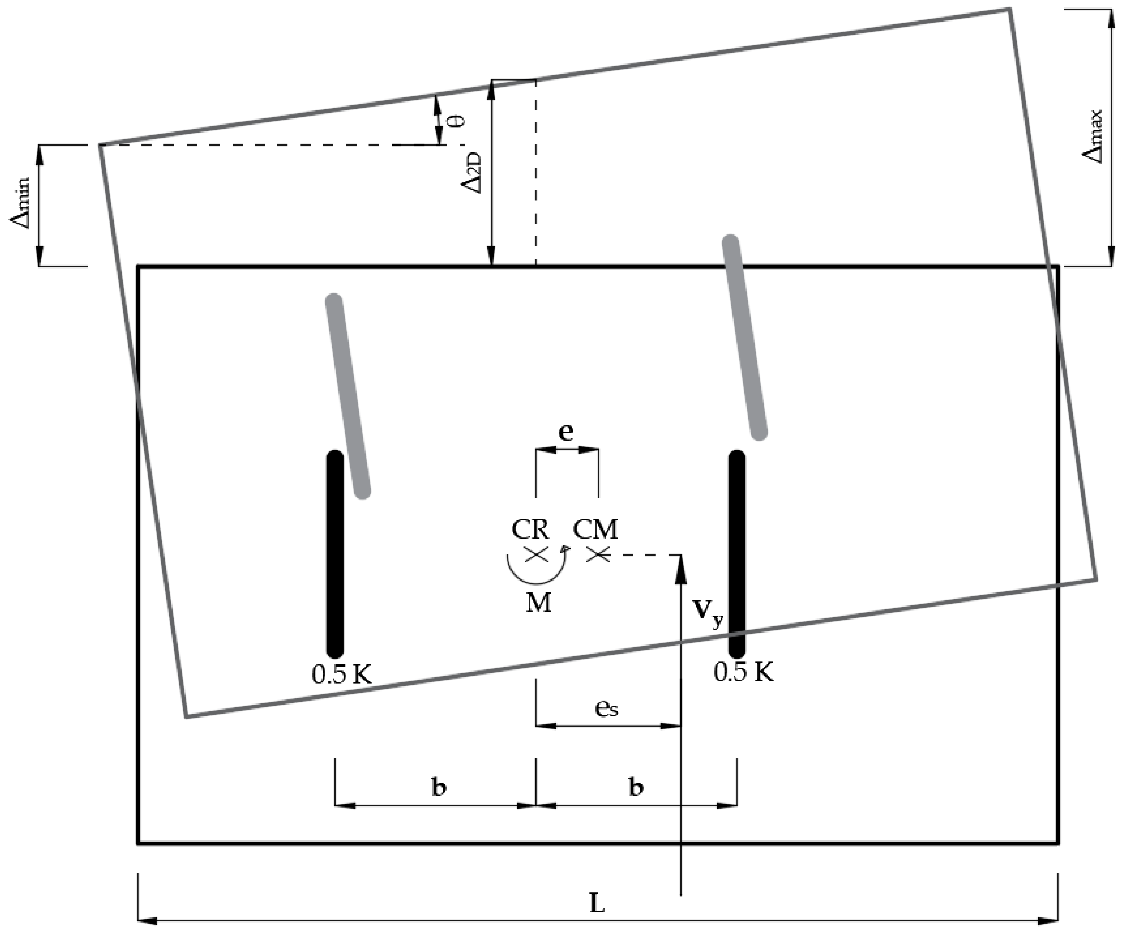
The elastic radius ratio (br) is defined as the square root of the ratio of torsional stiffness to translational stiffness of the building, normalised with respect to the mass radius of gyration (r) as presented in Equation (9). Its physical meaning is explained herein. The lateral load resisting elements of an asymmetrical building can always be idealised as a hypothetical “frame pair” with each frame having equal lateral translational stiffness of 0.5K (where K is the total lateral translational stiffness of the building), positioned at an equal distance away from the centre of rigidity (CR) as represented in Figure 6. Considering the hypothetical frame pair, the elastic radius (b) can be defined as the distance between the CR of the building and the frame. In other words, the pair of frames are spaced at a distance of 2b apart. This means that the larger the value of the elastic radius (b), the higher the torsional rigidity of the building as a whole.
Given that load V is applied at an offset “es” from the CR, the torsional moment is accordingly equal to V es. The torsional and translational stiffness of the building is accordingly obtained using Equations (10) and (11).
where and angle of rotation θ can both be found by following the procedure that has been illustrated previously, and θ can be calculated using Equation (12).
On substituting Equations (10)–(12) into Equation (9), the value of br is also obtained:
where es is the offset of the statically applied lateral load measured from the CR (which is not to be confused with the definition of “e” as shown in Figure 6).
2.2. Simplified Method for Determining Edge Displacement Ratio
The maximum edge displacement of the multi-storey building (Δ3D) can be estimated by solving the dynamic equations of equilibrium of the idealised single-storey building model. The 3D to 2D displacement ratio for acceleration-, velocity- and displacement-controlled conditions is estimated using Equations (14)–(16), respectively. The acceleration-, velocity-, and displacement-controlled conditions have been defined in Section 2.1.2 and Figure 2. The details about these equations and their derivation are given in [4,5].
where
- Br is the distance from the CM to the edge with maximum displacement, normalised to r,
- θj is the rotational component of the eigenvector solutions to the dynamic equations of equilibrium determined by Equation (17),
- λj is the eigenvalue solutions determined by Equation (18), and
- PFj is the participation factor for mode j determined by Equation (19).
The three-tiered approach involving a quick, refined, and detailed assessment method was developed based on these equations. Details of the assessment methodology are as described in the rest of this section (Section 2.2.1, Section 2.2.2 and Section 2.2.3).
2.2.1. Quick Assessment Method
The quick method of assessment is a swift and simple method for estimating the upper limit of the drift demand at the edge of the building taking into considerations of torsional amplification. In this method, Equations (20)–(22) are used for determining the upper limit of the edge displacement ratio (Δ3D/Δ2D) based on Br. The drift at the edge of the building should be within the upper limit as inferred from this ratio and the lower limit as calculated from the 2D analysis of the building (i.e., taking the displacement ratio equal to unity). Equations (20)–(22) are developed by simplifying Equations (14)–(16) assuming that the building is torsionally stable (br > 1) and has an er value of 0.7. These assumptions are found valid by the authors [4] for most buildings.
For acceleration-controlled condition (Tn1 ≤ T1),
For velocity-controlled condition (T1 < Tn1 ≤ T2),
For displacement-controlled condition (Tn1 > T2),
A building may be deemed to have a br value greater than 1.0 if the core walls (or shear walls) are positioned well away from the CR of the building, meeting one of the following criteria [25]:
- A building with four or more core walls (or shear walls)
A building with four or more core walls (or shear walls) may be deemed to have a br value greater than 1.0.
- A building with three core walls (or shear walls)
A building that is braced by three core walls (or shear walls) with a separation distance between the two external walls equal to the width of the building may be deemed to have a br value greater than 1.0. Two walls that are located close to each other may only be counted as one wall in this context.
- A building with two core walls (or shear walls)
A building that has two core walls (or shear walls) with a separation distance between the two walls exceeding 2r (where r is the mass radius of gyration of the building) may be deemed to have a br value greater than 1.0.
2.2.2. Refined Assessment Method
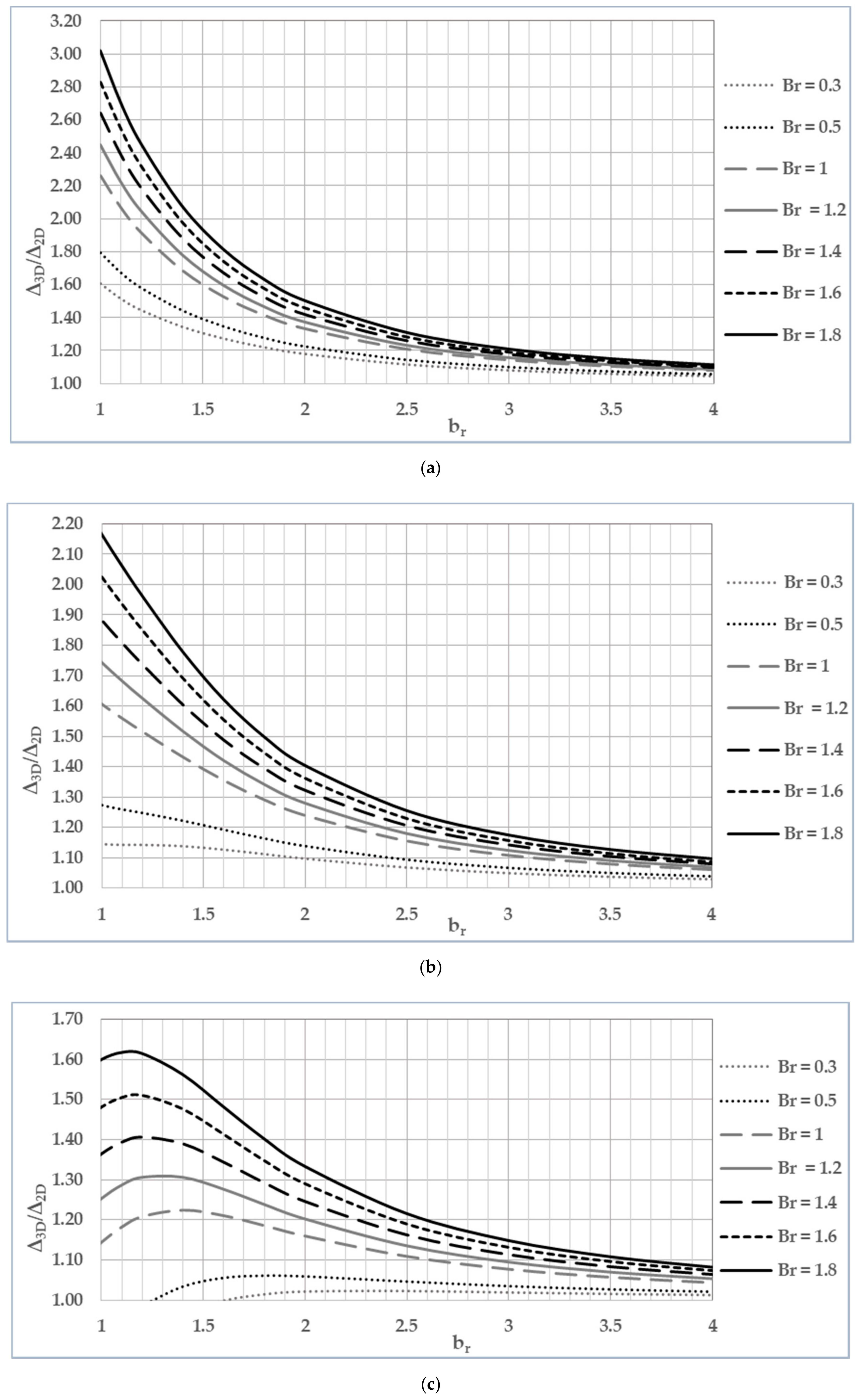
The refined method of assessment comprises three design charts, as presented in Figure 7 for predicting the 3D/2D displacement ratios. These graphs were derived from Equations (14)–(16) for the value of br ranging from 1 to 4, Br ranging from 0.3 to 1.8, and er of 0.7. In this method of assessment, the displacement ratio of the considered multi-storey building can be determined by first calculating the values of Br, br, and determining the controlling conditions as outlined in Section 2.1.1, Section 2.1.2, Section 2.1.3 and Section 2.1.4, and then directly reading the displacement ratio from the graphs presented in the design charts of Figure 7.
2.2.3. Detailed Estimation Method
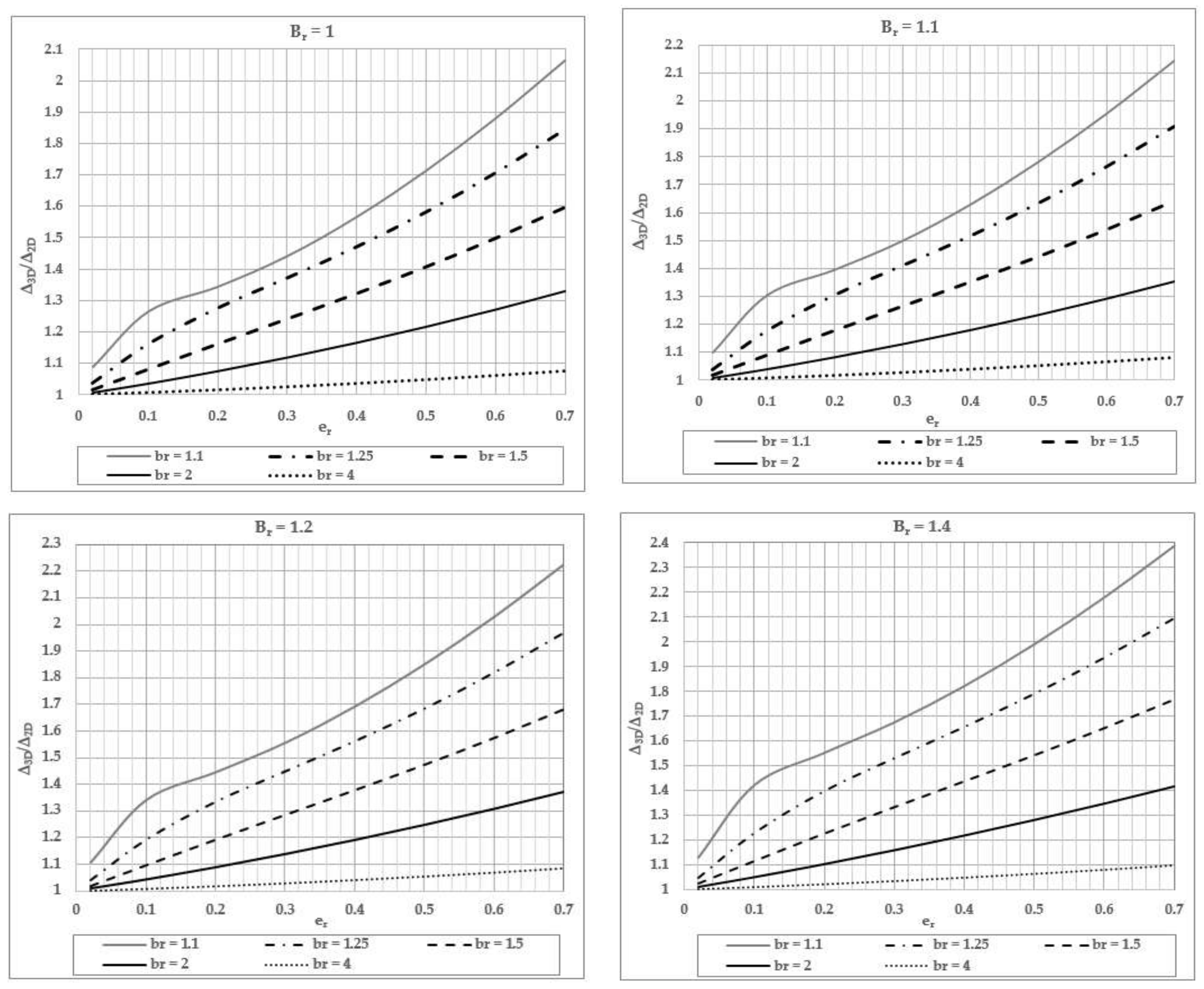
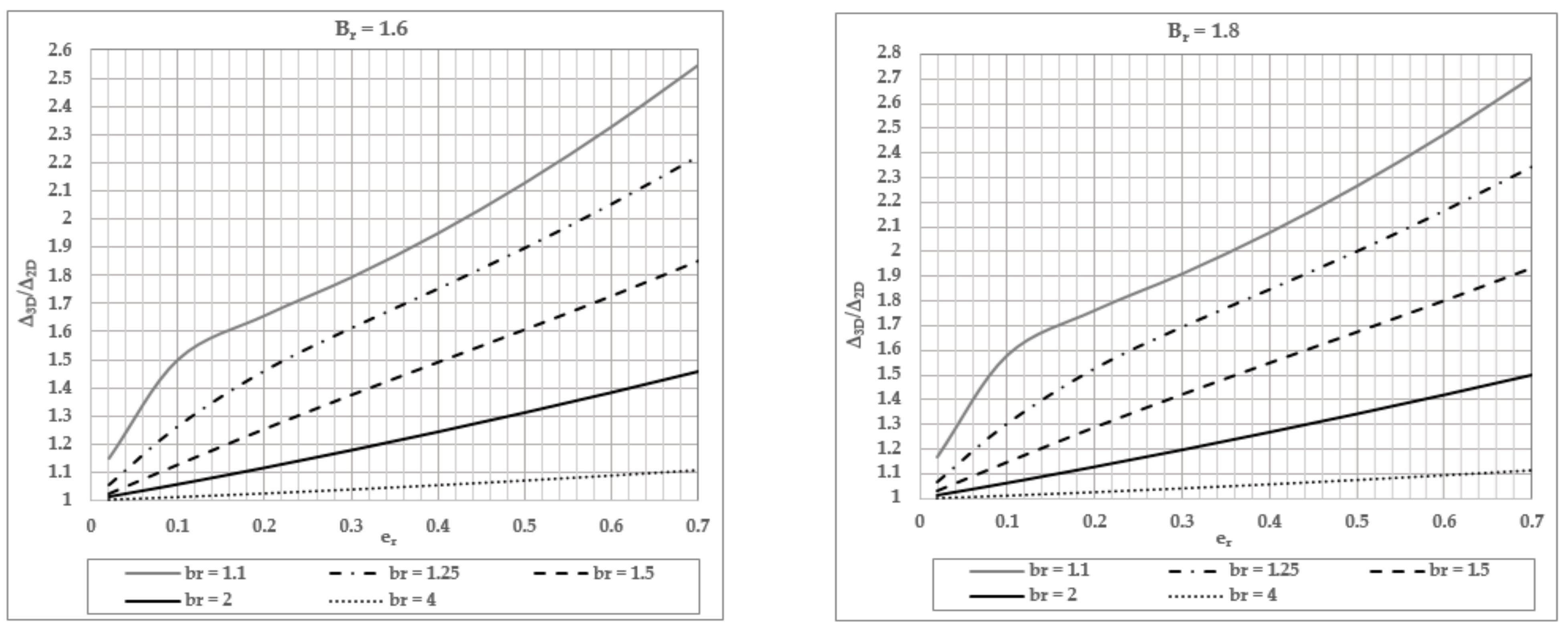
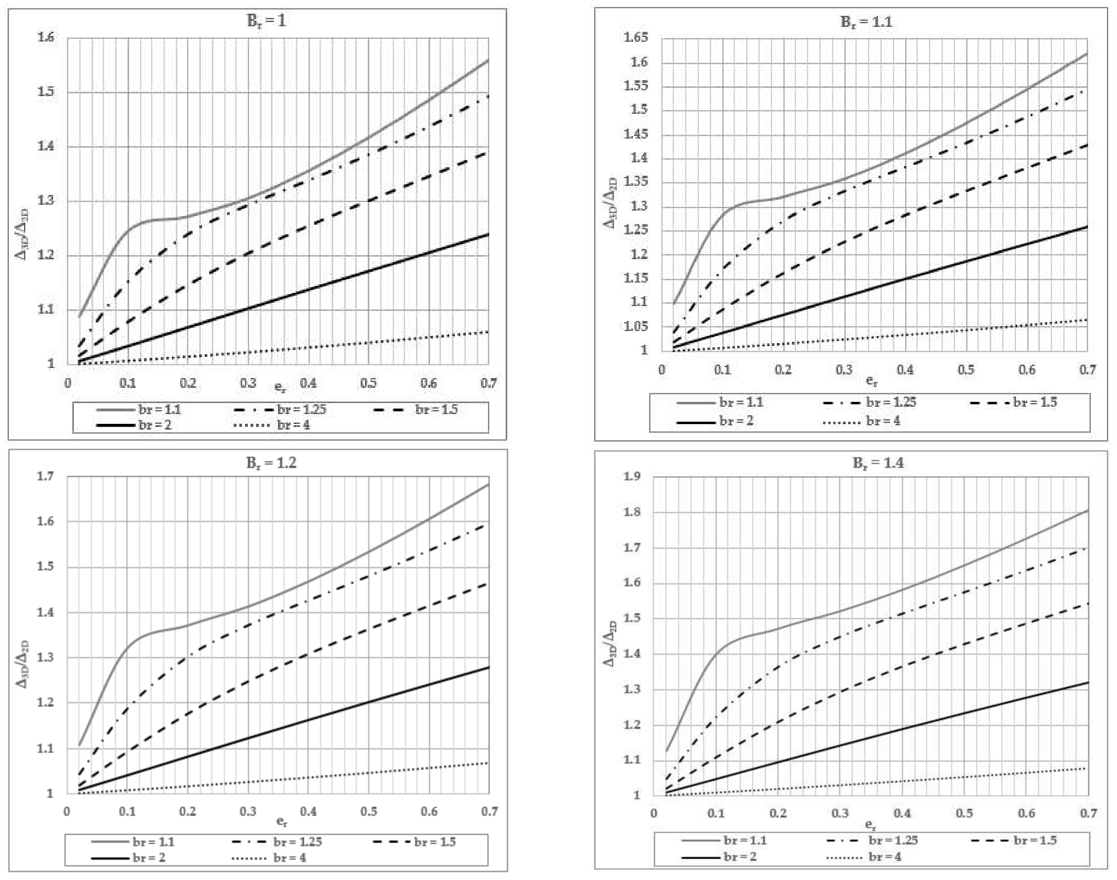
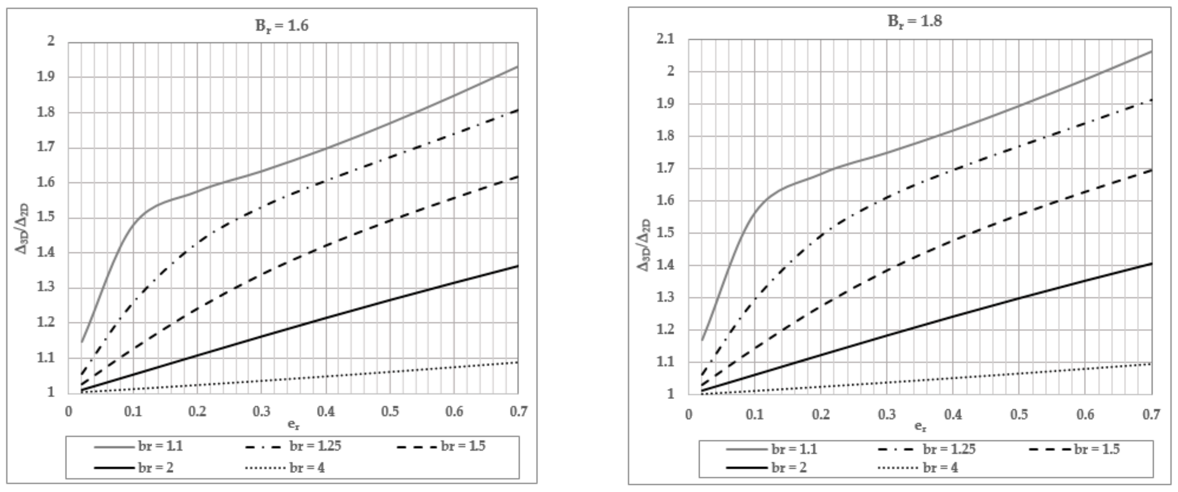
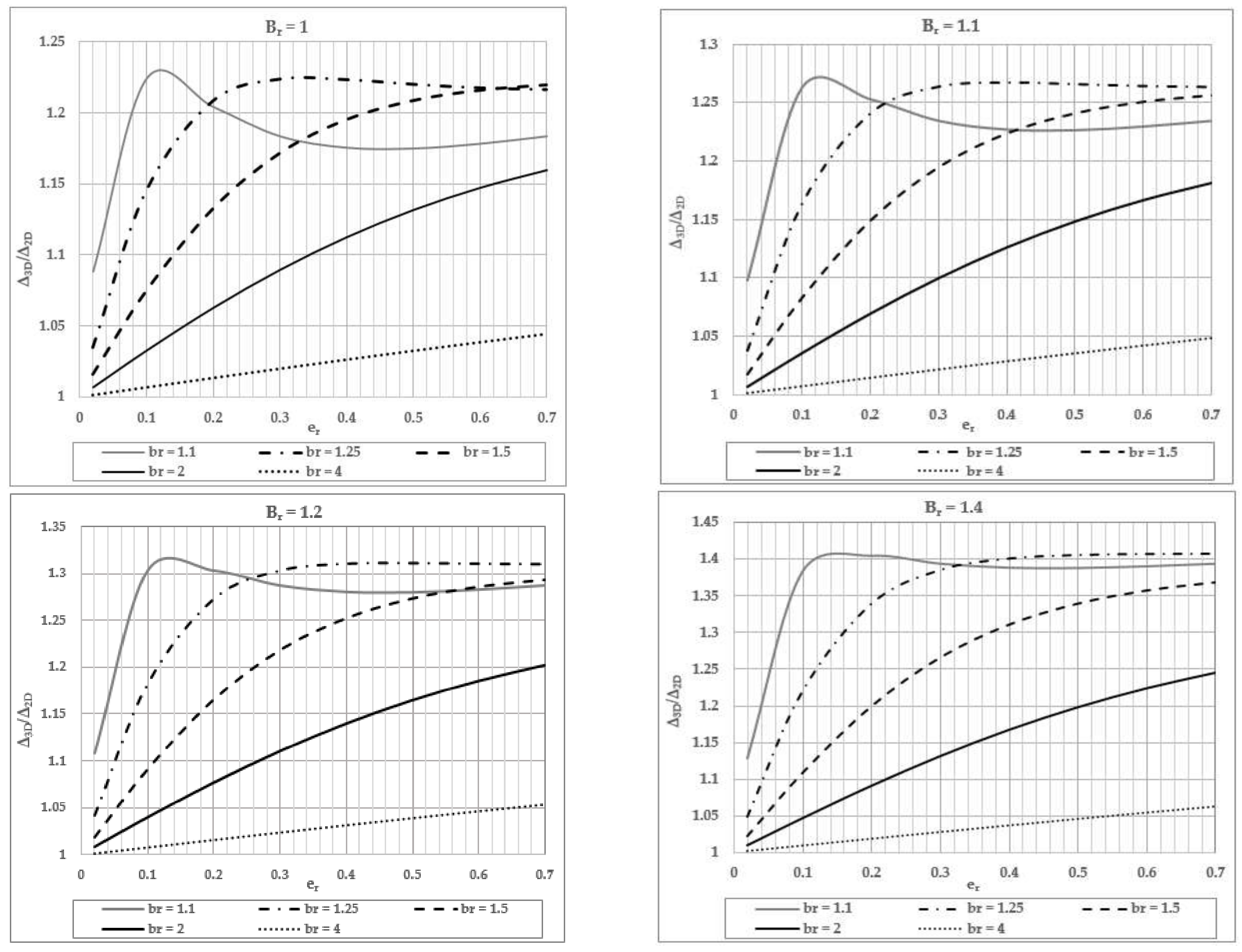
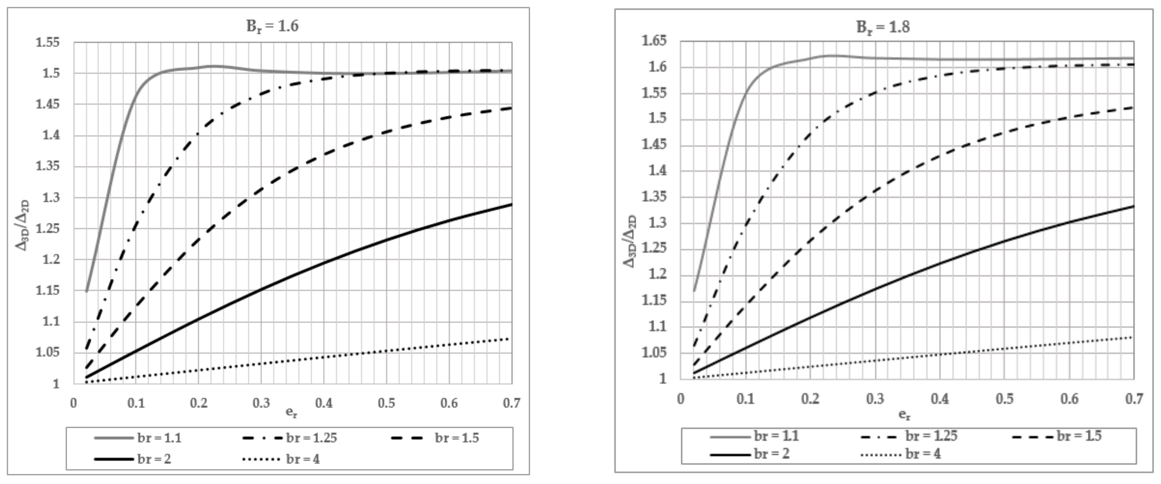
For the detailed method of assessment, three sets of design charts as presented in Figure 8, Figure 9 and Figure 10, which were derived from Equations (14)–(16) for the value of br ranging from 1.1 to 4, Br ranging from 1 to 1.8, and er ranging from 0.01 to 0.7. The edge displacement ratio for a multi-storey building can be found using Figure 8, Figure 9 and Figure 10, based on the values of Br, br, er, and the controlling conditions (refer Section 2.1.1, Section 2.1.2, Section 2.1.3 and Section 2.1.4).
3. Verification by Dynamic Analysis of Case Study Buildings
The developed method was verified by comparison with results from the dynamic analysis of six case study buildings. The analysis of the case study buildings was conducted using structural engineering software SPACE GASS (Version 12.85, SPACE GASS) [26]. The features of the six case study buildings are provided in this section.
Six case study buildings (CSB 1 to CSB 6) with the height ranging from 10 to 110 m were selected to test the reliability of the proposed methods in determining the edge displacement ratio of asymmetrical multi-storey buildings. The buildings were selected in such a way that the case studies can support the robustness of the proposed method for regular and irregular shaped buildings that are under acceleration-, velocity-, and displacement-controlled conditions and have a wide range of eccentricity. The structural floor plan of CSB 1-CSB 6 are presented in Figure 11, Figure 12, Figure 13, Figure 14, Figure 15 and Figure 16. As the purpose of the study is to compare the 3D and 2D displacements in the asymmetric buildings, the same general static and seismic loadings were considered. The imposed load of 2 kPa for typical floors and 0.25 kPa for the roof, superimposed dead load of 1 kPa for typical floor and 2.5 kPa for the roof, and façade load of 1 kPa were considered to determine the total storey dead and imposed loads following the Australian Standards [27]. Similarly, the seismic loading corresponding to the seismic hazard design factor (Z) of 0.08, probability factor (kp) of 1.8 (for 2500-year return period), and site sub-soil class of De was used in the analysis. Given that the analyses presented in the article were based on linear elastic behaviour, the 3D/2D amplification ratio should be independent on the intensity of the static loads and earthquake ground shaking. The geometrical and structural information of the case study buildings is presented in Table 1.
4. Results
The three methods of assessment as introduced in this paper: quick, refined, and detailed methods of assessment, for the calculation of edge displacement ratio (Δ3D/Δ2D), have been verified by the comparison of the model predictions with results from 3D dynamic analysis as performed using a commercial package such as SPACE GASS and the six case study buildings. Linear equivalent static analysis of the case study buildings was performed using SPACE GASS based on the horizontal equivalent static storey design forces determined as stipulated by current code provisions for seismic actions in Australia [30]. The seismic mass was calculated considering 100% of the dead load and 30% of the imposed load, and the horizontal storey forces were determined based on the seismic load as specified in Section 3. Following the determination of the horizontal storey forces, two linear static analysis were performed on each of the six case study buildings. A static analysis procedure as illustrated in Section 2.1.3 (following Method 1) was first employed to obtain the effective static 2D displacement (Δ2D) and the effective minimum and maximum edge displacements (Δmin and Δmax). The effective fundamental natural period of vibration (Tn1) of the case study buildings were calculated using Equation (2) based on the 2D quasi-static displacement profile presented in Figure 17. Finally, the torsional parameters Br (as per Section 2.1.1), br using Equation (13), and er using Equation (8) were determined. Results of the effective displacement, natural period of vibration, and the torsional parameters: r, Br, br, and er of the six case study buildings are presented in Table 2 for the critical direction of seismic actions. An example calculation of these parameters for CSB 1 is provided in Appendix B.
The torsional parameters presented in Table 2 were used to calculate the edge displacement ratio (Δ3D/Δ2D) using the quick, refined, and detailed methods of assessment. For the “quick” method of assessment, Equations (20)–(22) were used to calculate the upper limit of the displacement ratio. With the “refined” and “detailed” methods of predicting the drift at the edge of the building, the displacement ratios were read off directly from the charts provided in Figure 7, Figure 8, Figure 9 and Figure 10, respectively. To verify the results, the displacement ratios are compared with results from the dynamic modal analysis of the case study buildings. The dynamic modal analysis was performed using SPACE GASS based on the design response spectrum of Class De site with seismic hazard design factor (Z) of 0.08 and probability factor (kp) of 1.8 as specified in [30]. The effective displacement ratio (Δ3D/Δ2D) determined from the dynamic analysis are compared in Table 3 with the displacement ratios estimated using the quick, refined, and detailed methods of assessment.
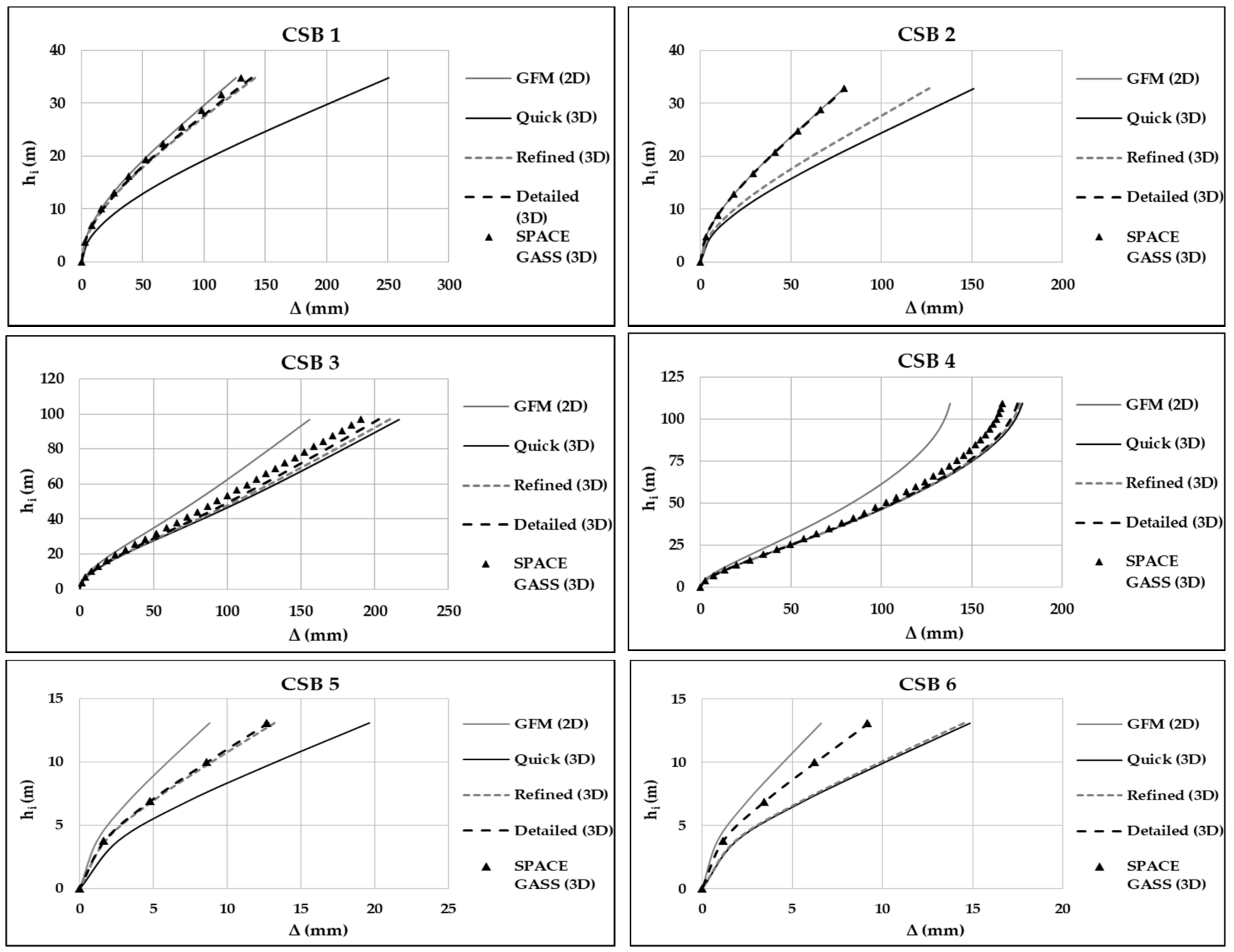
The maximum edge displacement demand values so obtained from the dynamic analysis are plotted against the height of the buildings and compared with the maximum edge displacement demand estimated using the proposed methods in Figure 18. Here, the maximum edge displacement values were estimated by multiplying the displacement of the equivalent 2D building from the dynamic analysis with the edge displacement ratio (Δ3D/Δ2D) values as presented in Table 3.
5. Discussion
The quick method of assessment allows the upper limit of the displacement ratio of an asymmetrical building to be determined for given dimensions of the floor plan (as represented by Br). This upper limit may be taken as a conservative estimate of the drift demand, and such an estimate can be made without the need of taking into account any detailed structural information of the building. As the quick method was derived in accordance with the most critical parameters, i.e., parameters that would result in the most erroneous displacement ratio values, the observed trend is expected. The estimates so obtained were found to be more conservative for low rise building (CSB 5 and CSB 6) and velocity-controlled regions (CSB 1 and CSB 2) compared to medium and high-rise buildings (CSB 3 and 4). This is because the torsional behaviour of asymmetrical buildings in displacement-controlled conditions is less sensitive to changes in the value of the torsional parameters (er and br) compared to buildings in acceleration-controlled or velocity-controlled conditions (as demonstrated in Figure 7, Figure 8, Figure 9 and Figure 10). The quick assessment method is shown to provide more conservative estimates for building with larger br values (e.g., CSB 1) and for buildings with smaller eccentricities (e.g., CSB 2). The displacement ratios are shown to be affected by eccentricity as well as torsional rigidity of the buildings. The sensitivity of the displacement behaviour of asymmetrical buildings to these parameters has also been reported in earlier studies [6,10,11,13].
The refined method may be used when the br value of the building is known. The refined method is generally shown to provide estimates that are closer to results from dynamic analyses compared with results from the quick method. The refined method was found to be able to match the dynamic analysis results to a reasonable degree of accuracy for buildings with higher values of eccentricity er (CSB 1, 3, 4, 5). The observed trend is expected as the charts used in the refined method (Figure 4) were developed from the value of er of 0.7, which is considered to be the upper bound value of er based on a review conducted by the authors [31]. In general, the detailed method would provide the most accurate estimates of the displacement ratio compared to the quick and refined method. The detailed method requires the values of br, er, and hence the location of the CM of the multi-storey buildings, to be known.
From the comparative analysis of the case study buildings estimated using the proposed method and the results from the dynamic modal analysis, the developed method is shown to be able to provide reasonable estimates of the maximum edge displacement demand of the buildings. The robustness of the method in predicting the displacement demand of asymmetrical multi-storey buildings has been demonstrated.
6. Conclusions
This study aims to introduce a multi-tiered approach (quick, refined, and detailed methods of assessment) for determining the maximum displacement demand at the edges of a regular, or an irregular, multi-storey building. A choice of static analysis procedure was first presented to locate the centre of rigidity of the building. Once the location is found, the elastic radius ratio and the eccentricity ratio of the building can be found. The tiered methods of assessment that are based on these two parameters involve the use of simple equations and design charts to operate. The assessment models have been developed by deriving from results obtained from parametric studies of single-storey building models. The robustness of the proposed methodology has been tested by comparison with results from dynamic modal analyses of six case study multi-storey buildings with regular and irregular floor plans.
Given the observations from the comparative analyses, the following conclusions can be drawn:
- The quick method of assessment is shown to be able to provide estimates of the upper limit of the maximum edge displacement demand of the building without the need of taking into account detailed structural information of the building. This upper limit may be taken as a conservative estimate of the drift demand. The method was found to give more conservative estimates for low- and medium-rise buildings in the acceleration- and velocity-controlled region than for taller buildings.
- The refined method of assessment is shown to be able to provide estimates of the maximum edge displacement demand with a reasonable degree of accuracy. The method may be used regardless of whether the eccentricity of the building is known.
- The detailed method of assessment was found to give estimates of the maximum edge displacement demand of a wide range of multi-storey buildings, and is more accurate in comparison with the refined and quick method as demonstrated by the six case study buildings.
Author Contributions
Conceptualization, E.L. and N.L.; Data curation, P.K., D.L. and E.L.; Formal analysis, P.K.; Funding acquisition, N.L. and E.L.; Investigation, P.K.; Methodology, E.L. and N.L.; Project administration, N.L. and E.L.; Resources, D.L. and P.K.; Software, P.K.; Supervision, E.L., N.L. and D.L.; Validation, P.K. and E.L.; Visualization, D.L. and P.K.; Writing—original draft, P.K.; Writing—review & editing, P.K., E.L., N.L. and D.L. All authors have read and agreed to the published version of the manuscript.
Funding
The research was funded by the Commonwealth of Australia through the Cooperative Research Centre program: BNHCRC A9.
Institutional Review Board Statement
Not applicable.
Informed Consent Statement
Not applicable.
Data Availability Statement
The data presented in this study are available in the article.
Acknowledgments
The financial contribution of the Commonwealth Australia through the Cooperative Research Centre Program is gratefully acknowledged.
Conflicts of Interest
The authors declare no conflict of interest.
Appendix A
Appendix A.1. Coordinate Method
In the coordinate method, a non-self-intersecting closed area bounded by the floor plan of the building is considered, and the coordinates of each vertex of the floor plan are determined. Then, the total area (A) and coordinates of the centre of mass (cx, cy) of the building is calculated using Equations (A1) to (A3). Similarly, the area moments of inertia about two principle axis (Ix and Iy) of the building about the origin (0,0) is determined using Equations (A4) and (A5). The reference point is transformed from origin to CM and the area moments of inertia about the CM are determined using the parallel axis theorem. Similarly, the polar moment of inertia (Iz,CM) about the centre of mass (CM) is determined by using the perpendicular axis theorem, as shown in Equation (A6). Finally, the radius of gyration of the building (r) is determined using Equation (A7).
where xi and yi are the x-coordinate and y-coordinate of vertex i of the building.
Appendix A.2. Calculation of Radius of Gyration of Case Study Building 5 Using Coordinate Method
The vertices in the floor plan of the case study building 5 (CSB 5) are numbered from 1 to 8 as shown in Figure A1, and the values of the coordinates along with parameters required for Equations (A1)–(A7) are shown in Table A1.
Figure A1.
CSB 5 with vertices number represented by numbers in red colour.


Table A1.
Coordinates of the vertices of the case study building 5 and calculation of the parameters required to determine the mass radius of gyration.
Table A1.
Coordinates of the vertices of the case study building 5 and calculation of the parameters required to determine the mass radius of gyration.
| No. | xi | yi | xi yi+1 − xi+1 yi | (xi yi+1 − xi+1 yi) | (xi yi+1 − xi+1 yi) | (xi2 + xi xi+1 + xi+12) (xi yi+1 − xi+1 yi) | (yi2 + yi yi+1 + yi+12) (xi yi+1 − xi+1 yi) |
|---|---|---|---|---|---|---|---|
| 1 | 0 | 0 | 0 | 0 | 0 | 0 | 0 |
| 2 | 48 | 0 | 1186 | 113,818 | 29,284 | 8,194,867 | 723,323 |
| 3 | 48 | 24.7 | 1186 | 56,909 | 58,569 | 2,731,622 | 2,169,968 |
| 4 | 0 | 24.7 | 0 | 0 | 0 | 0 | 0 |
| 5 | 0 | 16.55 | −662 | −26,480 | −21,912 | −1,059,200 | −543,970 |
| 6 | 40 | 16.55 | −336 | −26,880 | −8299 | −1,612,800 | −159,670 |
| 7 | 40 | 8.15 | 326 | 13,040 | 5314 | 521,600 | 64,961 |
| 8 | 0 | 8.15 | 0 | 0 | 0 | 0 | 0 |
| 1 | 0 | 0 | - | - | - | - | - |
| Sum= | 1699 | 130,406 | 62,955 | 8,776,090 | 2,254,612 |
Now, the sum of five quantities from Table A1 is used in Equations (A1)–(A7) to calculate the total area, coordinates of CM, area moment of inertia, polar moment of inertia, and radius of gyration.
Appendix B. Example Calculation of Torsional Parameters and Displacement Ratio for CSB 1
The storey height and mass, equivalent static storey design forces determined as per AS 1170.4 (2007), and the static storey displacements determined from SPACE GASS are summarised in Table A2. Using Equation (4) and the sum of quantities mi δ2D,i and mi δ2D,i2 from Table A2, the value of Δ2D is determined as follows,
Similarly, the value of Δmin and Δmax are calculated as 161.23 mm and 196.89 mm, respectively.
Table A2.
Detail of the storey height (hi), storey mass (mi), and equivalent static storey design forces (Fi) of the case study building 1 (CSB 1).
Table A2.
Detail of the storey height (hi), storey mass (mi), and equivalent static storey design forces (Fi) of the case study building 1 (CSB 1).
| Level | hi (m) | mi (t) | Fi (kN) | δ2D,i (mm) | δmin,i (mm) | δmax,i (mm) | ||
|---|---|---|---|---|---|---|---|---|
| Roof | 34.8 | 848 | 5299 | 246 | 230 | 273 | 208,176 | 51,118,670 |
| 10 | 31.7 | 838 | 4685 | 215 | 202 | 239 | 180,385 | 38,818,861 |
| 9 | 28.6 | 838 | 4142 | 185 | 173 | 206 | 155,086 | 28,693,908 |
| 8 | 25.5 | 838 | 3610 | 155 | 145 | 172 | 130,168 | 20,214,048 |
| 7 | 22.4 | 838 | 3091 | 126 | 118 | 140 | 105,964 | 13,395,584 |
| 6 | 19.3 | 838 | 2586 | 99 | 93 | 110 | 82,906 | 8,199,957 |
| 5 | 16.2 | 838 | 2097 | 73 | 69 | 81 | 61,487 | 4,510,325 |
| 4 | 13.1 | 838 | 1626 | 50 | 47 | 56 | 42,265 | 2,131,092 |
| 3 | 10 | 838 | 1177 | 31 | 29 | 34 | 25,859 | 797,779 |
| 2 | 6.9 | 838 | 754 | 15 | 14 | 17 | 12,910 | 198,840 |
| 1 | 3.8 | 874 | 385 | 5 | 5 | 5 | 4285 | 20,994 |
| Sum | 9266 | 29,452 | - | - | - | 1,009,491 | 168,100,058 | |
By substituting the values of total base shear (Vb = sum of Fi) and the sum of mi δ2D,i (from Table A2) in Equation (2), the value of effective fundamental natural period (Tn1) is calculated as:
Now, using AutoCAD, the value of B of 26.91 m (from the flexible edge) and the radius of gyration of 15.86 m was obtained. From the value of B and r, the value of Br is calculated as:
Now, substituting the values of effective displacements and the length of the building (43 m for motion about the x-axis), the position of the centre of rigidity (CR) is determined as:
Then, the value of normalised eccentricity (er) is determined from the positions of CM and CR relative to the stiff edge of the building,
Similarly, the value of es (distance from CR to the position of applied load) is determined as shown below,
Now, the value of br is calculated as follows,
Finally, the value of the displacement ratios are determined using quick, refined, and detailed estimate methods:
- Quick estimate: As the building is in velocity controlled condition (T1 = 0.3 s < Tn1 = 1.16 s ≤ T2 = 1.5 s), the displacement ratio can be calculated using Equation (21),
- Refined estimate: For velocity controlled conditions, Br = 1.7 and br = 3.34, the displacement ratio can be read from Figure 7 as 1.3.
- Detailed estimate: For velocity controlled conditions, Br = 1.7, br = 3.34, and er = 0.61, the displacement ratio can be read from Figure 9 as 1.1.
References
- Lumantarna, E.; Menegon, S.J.; Lam, N.; Wilson, J. Simplified approach for multi-storey asymmetrical buildings in regions of low to moderate seismicity. Australas. Struct. Eng. Conf. 2020. accepted. [Google Scholar]
- Westenenk, B.; de la Llera, J.C.; Jünemann, R.; Hube, M.A.; Besa, J.J.; Lüders, C.; Inaudi, J.A.; Riddell, R.; Jordán, R. Analysis and interpretation of the seismic response of RC buildings in Concepción during the February 27, 2010, Chile earthquake. Bull. Earthq. Eng. 2013, 11, 69–91. [Google Scholar] [CrossRef]
- Wilson, J.; Lam, N.T.K.L. Earthquake design of buildings in Australia using velocity and displacement principles. Aust. J. Struct. Eng. 2006, 6, 103–118. [Google Scholar] [CrossRef]
- Lumantarna, E.; Lam, N.; Wilson, J. Methods of analysis for buildings with uni-axial and bi-axial asymmetry in regions of lower seismicity. Earthq. Struct. 2018, 15, 81–95. [Google Scholar]
- Lam, N.T.; Wilson, J.L.; Lumantarna, E. Simplified elastic design checks for torsionally balanced and unbalanced low-medium rise buildings in lower seismicity regions. Earthq. Struct. 2016, 11, 741–777. [Google Scholar] [CrossRef]
- Anagnostopoulos, S.A.; Kyrkos, M.T.; Stathopoulos, K.G. Earthquake induced torsion in buildings: Critical review and state of the art. Earthq. Struct. 2015, 8, 305–377. [Google Scholar] [CrossRef] [Green Version]
- Mohamed, O.A.; Mehana, M.S. Assessment of Accidental Torsion in Building Structures Using Static and Dynamic Analysis Procedures. Appl. Sci. 2020, 10, 5509. [Google Scholar] [CrossRef]
- Tscinias, T.G.; Hutchinson, G.L. Evaluation of code requirements for the earthquake resistant design of torsionally coupled buildings. Proc. Inst. Civ. Eng. 1981, 71, 821–843. [Google Scholar]
- Dempsey, K.M.; Tso, W.K. An alternative path to seismic torsional provisions. Soil Dyn. Earthq. Eng. 1982, 1, 3–10. [Google Scholar] [CrossRef]
- Chandler, A.M.; Hutchinson, G.L. A modified approach to earthquake resistant design of torsionally coupled buildings. Bull. N. Z. Natl. Soc. Earthq. Eng. 1988, 21, 140–152. [Google Scholar] [CrossRef]
- Rutenberg, A.; Pekau, O.A. Seismic code provisions for asymmetric structures: Low period systems. Eng. Struct. 1989, 11, 92–96. [Google Scholar] [CrossRef]
- Balendra, T.; Lam, N.T.K.; Perry, M.J.; Lumantarna, E.; Wilson, J.L. Simplified displacement demand prediction of tall asymmetric buildings subjected to long-distance earthquakes. Eng. Struct. 2005, 27, 335–348. [Google Scholar] [CrossRef]
- Lumantarna, E.; Lam, N.; Wilson, J. Displacement-Controlled Behavior of Asymmetrical Single-Story Building Models. J. Earthq. Eng. 2013, 17, 902–917. [Google Scholar] [CrossRef]
- Tso, W.K.; Zhu, T.J. Design of torsionally unbalanced structural systems based on code provisions I: Ductility demand. Earthq. Eng. Struct. Dyn. 1992, 21, 609–627. [Google Scholar] [CrossRef]
- Chandler, A.M.; Duan, X.N. Performance of asymmetric code-designed buildings for serviceability and ultimate limit states. Earthq. Eng. Struct. Dyn. 1997, 26, 717–735. [Google Scholar] [CrossRef]
- Stathopoulos, K.G.; Anagnostopoulos, S.A. Accidental design eccentricity: Is it important for the inelastic response of buildings to strong earthquakes? Soil Dyn. Earthq. Eng. 2010, 30, 782–797. [Google Scholar] [CrossRef]
- Gasparini, G.; Silvestri, S.; Trombetti, T. A simple code-like formula for estimating the torsional effects on structures subjected to earthquake ground motion excitation. In Proceedings of the 14th World Conference on Earthquake Engineering, Beijing, China, 12–17 October 2008. [Google Scholar]
- Trombetti, T.; Palermo, M.; Silvestri, S.; Gasparini, G. Period shifting effect on the corner displacement magnification of one-storey asymmetric systems. In Proceedings of the 15th World Conference on Earthquake Engineering, Lisbon, Portugal, 24–28 September 2012. [Google Scholar]
- EN 1998-1. Eurocode 8: Design of Structures for Earthquake Resistance—Part 1: General Rules, Seismic Actions and Rules for Buildings; European Committee for Standardization: Brussels, Belgium, 2005.
- FEMA. Prestandard and Commentary for the Seismic Rehabilitation of Buildings (FEMA356); Federal Emergency Management Agency: Washington, DC, USA, 2000.
- Building Seismic Safety Council. NEHRP Recommended Provisions for Seismic Regulations for New Buildings and Other Structures Part 1: Provisions (FEMA450); National Institute of Building Sciences: Washington, DC, USA, 2003.
- Lumantarna, E.; Mehdipanah, A.; Lam, N.; Wilson, J. Methods of structural analysis of buildings in regions of low to moderate seismicity. In Proceedings of the 2017 World Congress on Advances in Structural Engineering and Mechanics (ASEM17), Ilsan, Seoul, Korea, 28 August–1 September 2017. [Google Scholar]
- Khatiwada, P. Determination of center of mass and radius of gyration of irregular buildings and its application in torsional analysis. Int. Res. J. Eng. Technol. 2020, 7, 1–7. [Google Scholar]
- MASSPROP (Command). Available online: https://knowledge.autodesk.com/support/autocad/learn-explore/caas/CloudHelp/cloudhelp/2020/ENU/AutoCAD-Core/files/GUID-CAA51229-293E-4A0C-BFF3-93226252CF13-htm.html (accessed on 21 November 2020).
- Xing, B.; Lumantarna, E.; Lam, N.T.K.; Menegon, S. Evaluation of torsional effects on reinforced concrete buildings due to the excitation of an earthquake. In Proceedings of the Australian Earthquake Engineering Society Virtual Conference, Melbourne, VIC, Australia, 25−27 November 2016. [Google Scholar]
- SPACE GASS. Documentation for the SPACE GASS Structural Engineering Design and Analysis Software; SPACE GASS: Geelong, VIC, Australia, 2005. [Google Scholar]
- Australian Standard. AS 1170.1-2002. Structural Design Actions, Part 1: Permanent, Imposed and Other Actions; Standards New Zealand: Wellington, New Zealand, 2002. [Google Scholar]
- Menegon, S.J.; Tsang, H.H.; Lumantarna, E.; Lam, N.T.K.; Wilson, J.L.; Gad, E.F. Framework for seismic vulnerability assessment of reinforced concrete buildings in Australia. Aust. J. Struct. Eng. 2019, 20, 143–158. [Google Scholar] [CrossRef]
- Shan, Z.W.; Looi, D.T.W.; Cheng, B.; Su, R.K.L. Simplified seismic axial collapse capacity prediction model for moderately compressed RC shear walls adjacent to transfer structure in tall buildings. Struct. Des. Tall Spec. Build. 2020, 29, e1752. [Google Scholar] [CrossRef]
- Australian Standard. AS 1170.4-2007. Structural Design Actions, Part 4: Earthquake Actions in Australia; Australian Standard: Sydney, NSW, Australia, 2007. [Google Scholar]
- Lumantarna, E.; Lam, N.; Wilson, J. Predicting Maximum Displacement Demand of Asymmetric Reinforced Concrete Buildings; Australian Earthquake Engineering Society: Newcastle, NSW, Australia, 2019. [Google Scholar]
Figure 1.
The radius of gyration (r) and distance between the centre of mass (CM) and furthest structural elements (Bx,1, Bx,2, By,1, and By,2) about the two principal directions (x and y) in the irregular building.
Figure 1.
The radius of gyration (r) and distance between the centre of mass (CM) and furthest structural elements (Bx,1, Bx,2, By,1, and By,2) about the two principal directions (x and y) in the irregular building.

Figure 2.
Response spectral displacement diagram with acceleration, velocity, and displacement controlled conditions delimited by the first corner period (T1) and the second corner period (T2).
Figure 2.
Response spectral displacement diagram with acceleration, velocity, and displacement controlled conditions delimited by the first corner period (T1) and the second corner period (T2).

Figure 3.
Method 1 of locating the centre of rigidity (CR) based on analysis of torsionally restrained and unrestrained building models.
Figure 3.
Method 1 of locating the centre of rigidity (CR) based on analysis of torsionally restrained and unrestrained building models.

Figure 4.
Method 2 of locating the CR based on 3D analyses and extrapolation.

Figure 5.
Method 3 of locating the CR based on 3D analyses and interpolation.

Figure 6.
Detail of the frame pair (thick dark bands) and its spacing (b) in a rectangular building. Rotation of the frame pair and the building (final shape in grey colour) by angle θ on applying the lateral load V at a distance of es from the centre of rigidity (CR).
Figure 6.
Detail of the frame pair (thick dark bands) and its spacing (b) in a rectangular building. Rotation of the frame pair and the building (final shape in grey colour) by angle θ on applying the lateral load V at a distance of es from the centre of rigidity (CR).

Figure 7.
3D to 2D displacement ratio: (a) acceleration-controlled condition (Tn1 ≤ T1); (b) velocity-controlled condition (T1 < Tn1 ≤ T2); and (c) displacement-controlled condition (Tn1 > T2).
Figure 7.
3D to 2D displacement ratio: (a) acceleration-controlled condition (Tn1 ≤ T1); (b) velocity-controlled condition (T1 < Tn1 ≤ T2); and (c) displacement-controlled condition (Tn1 > T2).

Figure 8.
Edge displacement ratio for acceleration-controlled condition (Tn1 ≤ T1).


Figure 9.
Edge 3D to 2D displacement ratio for velocity-controlled condition (T1 < Tn1 ≤ T2).


Figure 10.
Edge displacement ratio for displacement-controlled condition (Tn1 > T2).


Figure 11.
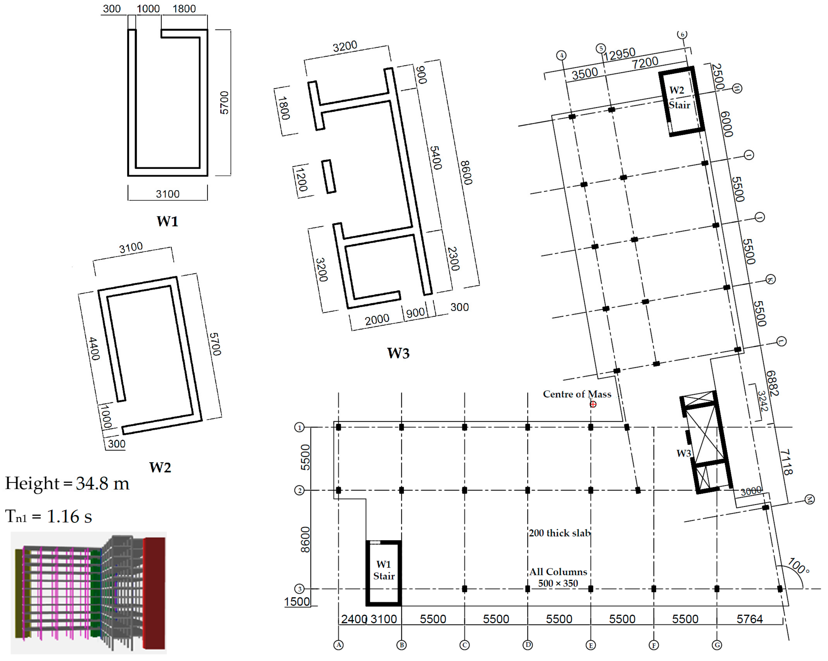
Floor plan, structural layout, and elevation view of CSB 1 (all dimensions are in mm) [28].
Figure 11.
Floor plan, structural layout, and elevation view of CSB 1 (all dimensions are in mm) [28].

Figure 12.
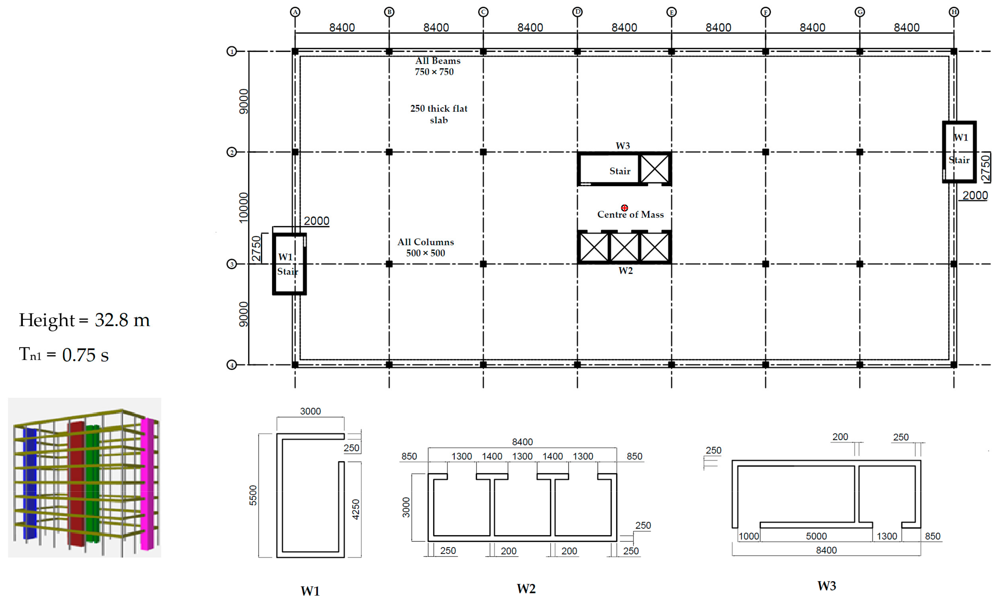
Floor plan, structural layout, and elevation view of CSB 2 (all dimensions are in mm) [28].
Figure 12.
Floor plan, structural layout, and elevation view of CSB 2 (all dimensions are in mm) [28].

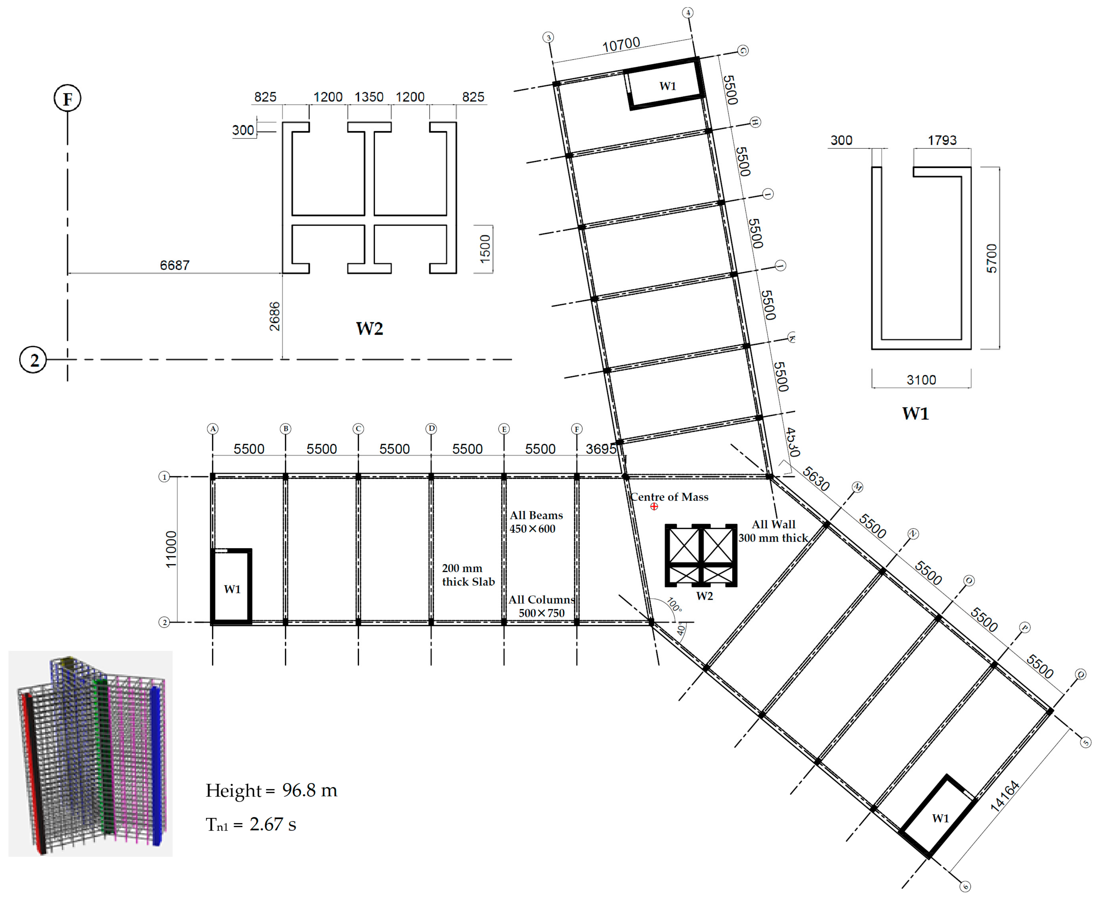
Figure 13.
Floor plan, structural layout, and elevation view of CSB 3 (all dimensions are in mm).

Figure 14.
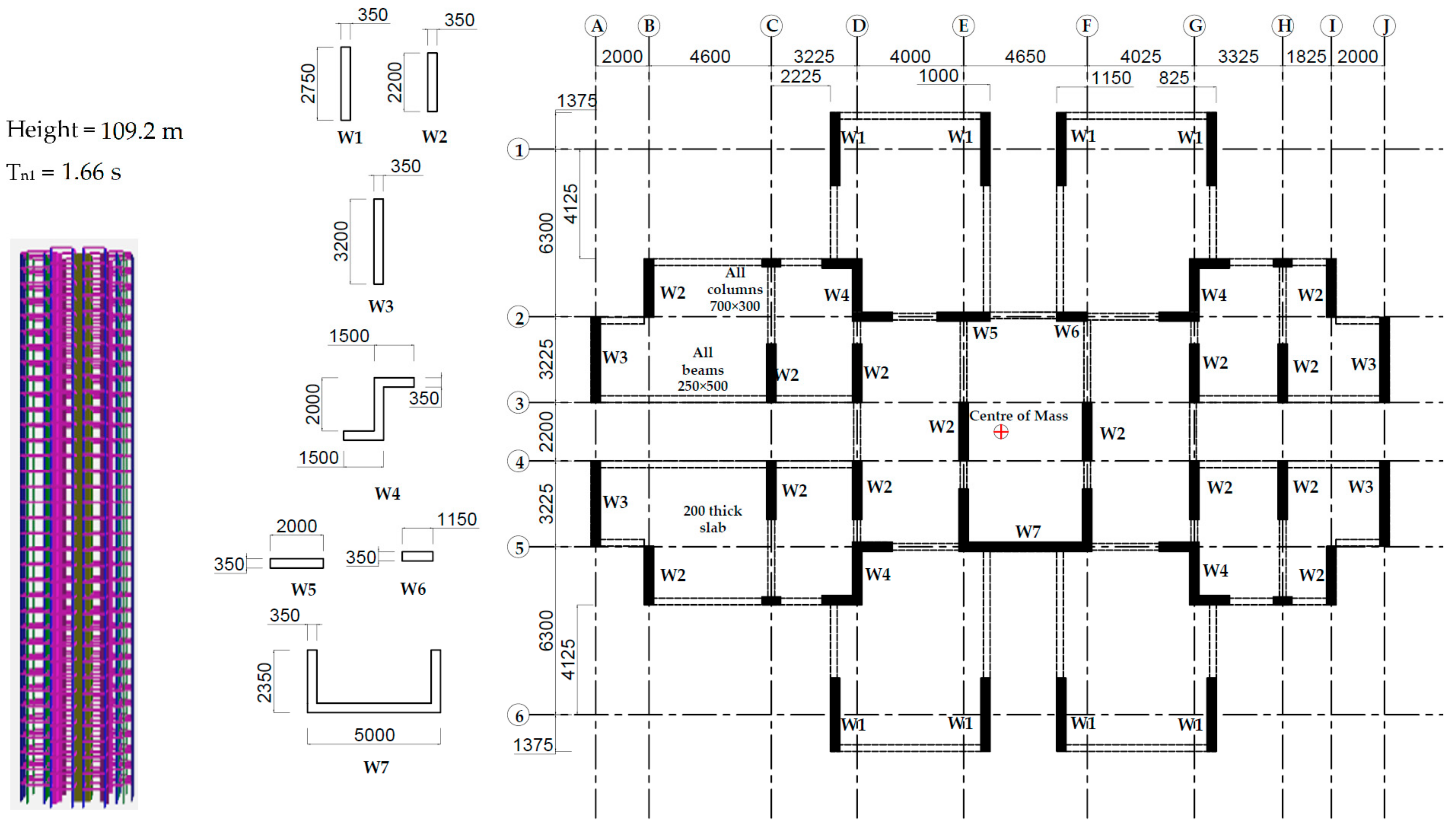
Floor plan, structural layout, and elevation view of CSB 4 (all dimensions are in mm) [29].
Figure 14.
Floor plan, structural layout, and elevation view of CSB 4 (all dimensions are in mm) [29].

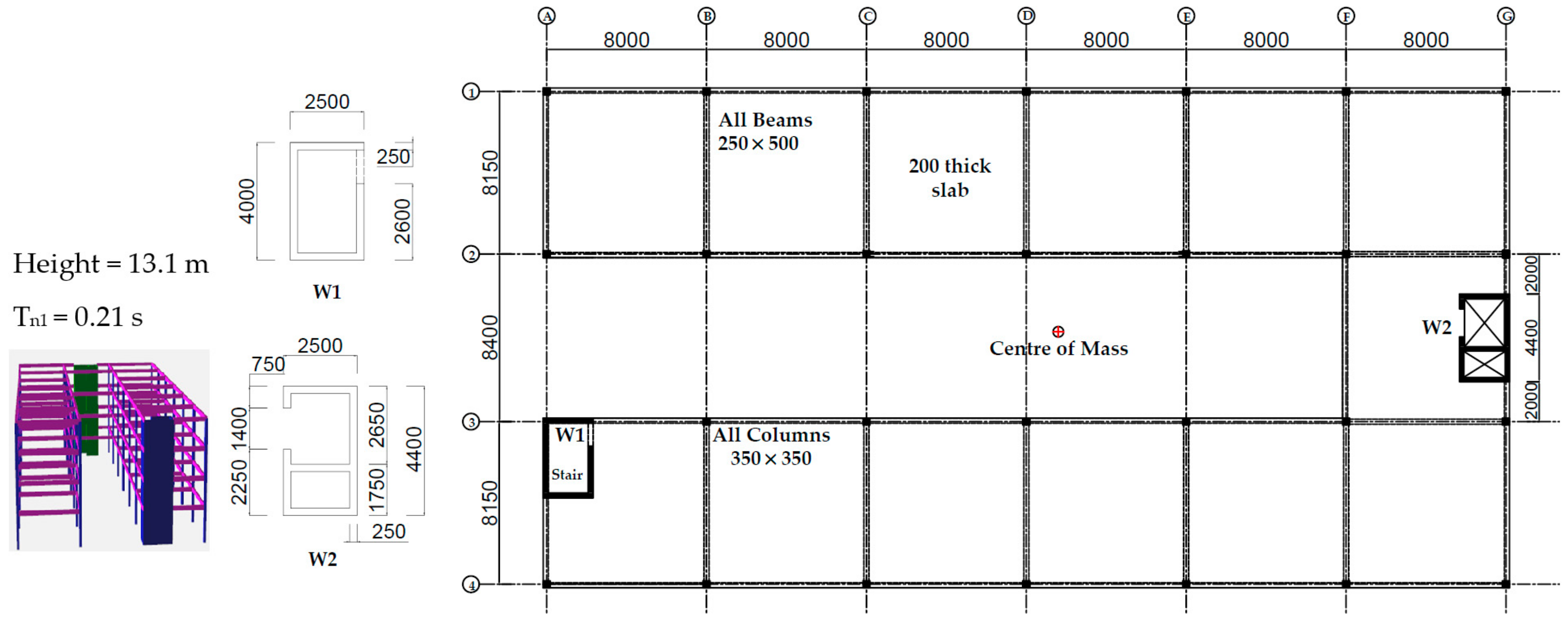
Figure 15.
Floor plan, structural layout, and elevation view of CSB 5 (all dimensions are in mm).

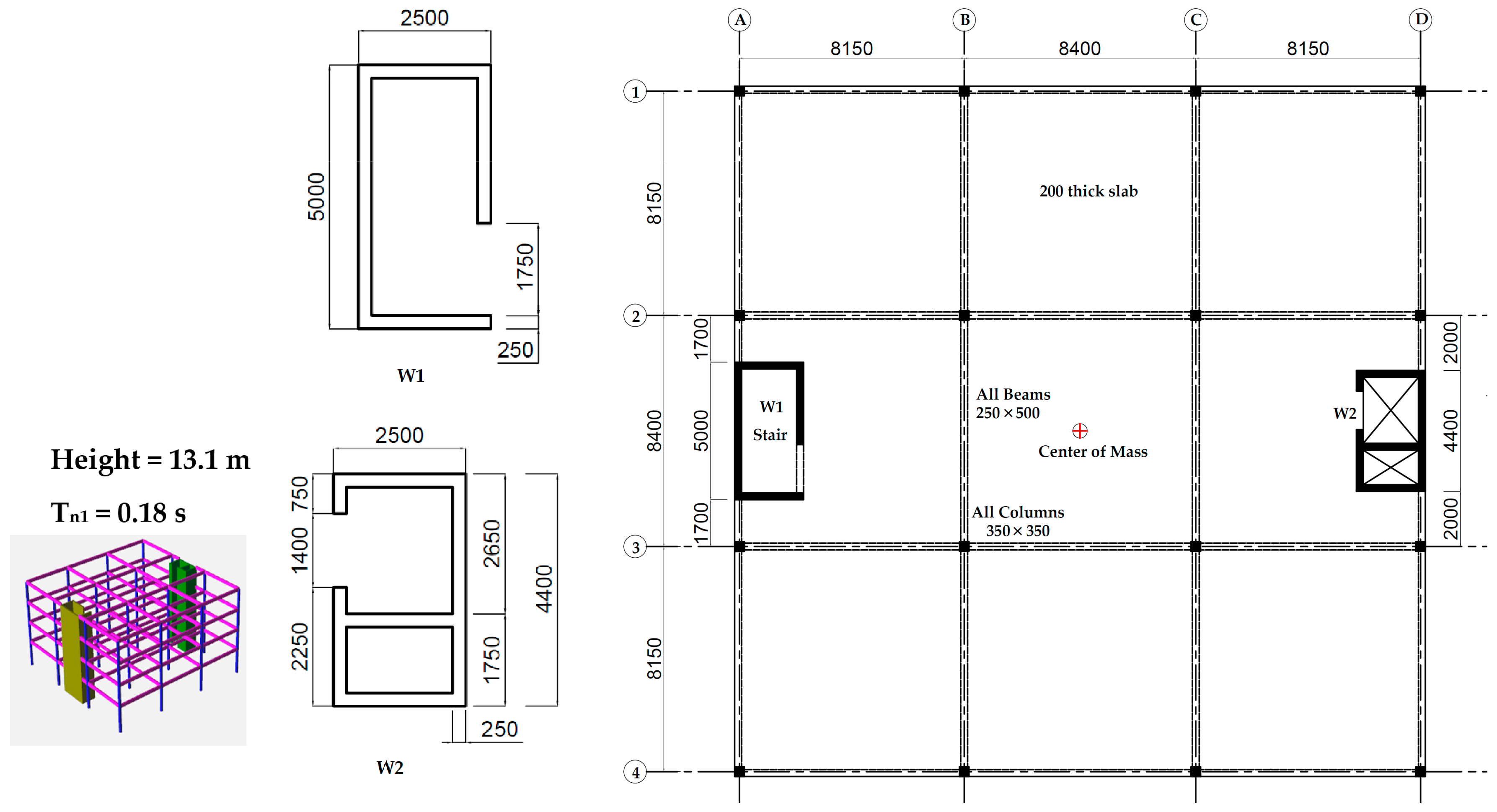
Figure 16.
Floor plan, structural layout, and elevation view of CSB 6 (all dimensions are in mm).

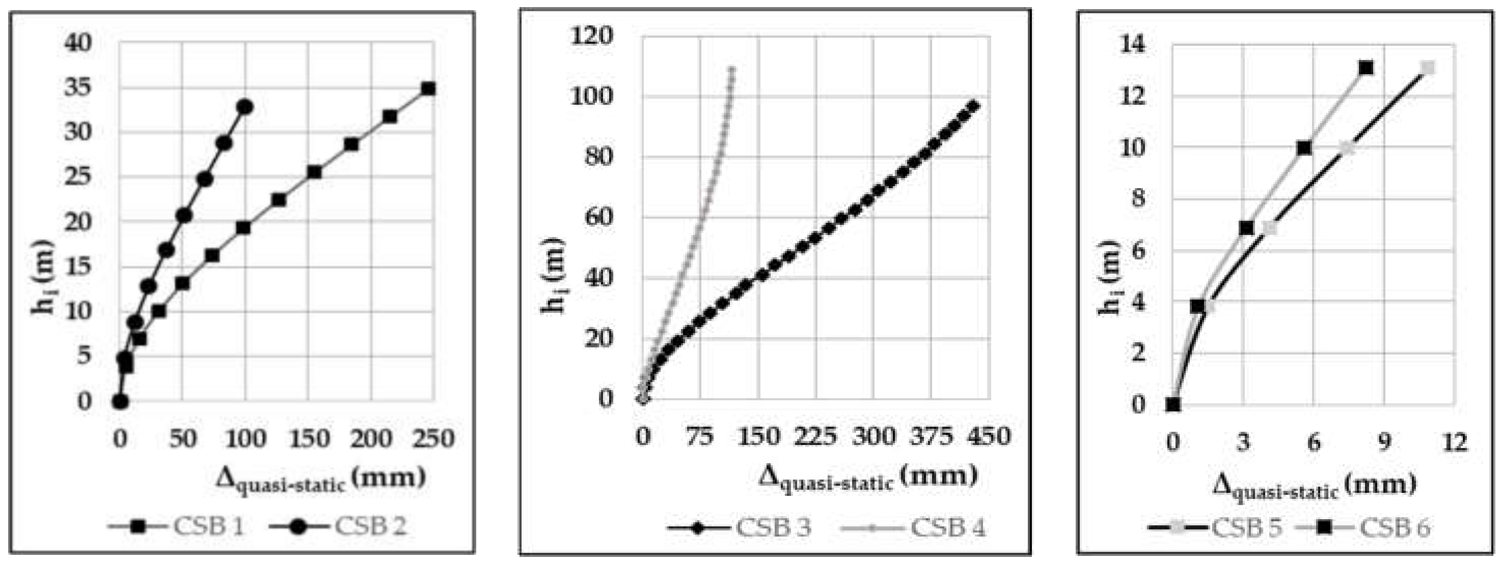
Figure 17.
2D quasi-static displacement profiles of the case study buildings obtained from SPACE GASS (by applying horizontal equivalent static design forces calculated as per [30]).
Figure 17.
2D quasi-static displacement profiles of the case study buildings obtained from SPACE GASS (by applying horizontal equivalent static design forces calculated as per [30]).

Figure 18.
Comparison of the displacement profile of the 3D displacement of the case study buildings estimated by the developed method and results from SPACE GASS. The Generalised Force Method (GFM) (2D) displacement profile is obtained using the Generalised Force Method of analysis and is presented as a lower bound estimate. The method has been presented in an earlier study by the authors [5].

Table 1.
Geometrical and structural information of the case study buildings (CSB).
| CSB No. | No. of Storey, Height (m) | Shape | Regular/Irregular Plan | Length (m) × Width (m) | LLRS Type 1 |
|---|---|---|---|---|---|
| CSB 1 | 11, 34.8 | L | Irregular | 39 × 47 | Wall |
| CSB 2 | 8, 32.8 | Rectangular | Regular | 58.8 × 28 | Mixed 2 |
| CSB 3 | 31, 96.8 | Y | Irregular | 63.7 × 60.7 | Mixed |
| CSB 4 | 35, 109.2 | Cross | Irregular | 30 × 24 | Mixed |
| CSB 5 | 4, 13.1 | U | Irregular | 48 × 24.7 | Mixed |
| CSB 6 | 4, 13.1 | Square | Regular | 24.7 × 24.7 | Mixed |
1 LLRS type is the type of lateral load resisting system present in the case study buildings. 2 Mixed is LLRS type consisting of walls and moment-resisting frames.
Table 2.
Effective displacements, effective natural period, and torsional parameters of the six case study buildings (CSB) for the critical direction of seismic action.
Table 2.
Effective displacements, effective natural period, and torsional parameters of the six case study buildings (CSB) for the critical direction of seismic action.
| CSB | Δ2D (mm) | Δmin (mm) | Δmax (mm) | Tn1 (s) | r (m) | Br | br | er |
|---|---|---|---|---|---|---|---|---|
| CSB 1 | 166 | 161 | 197 | 1.16 | 15.86 | 1.7 | 3.34 | 0.61 |
| CSB 2 | 69 | 53 | 84 | 0.75 | 18.80 | 1.6 | 1.47 | 0.002 |
| CSB 3 | 299 | 165 | 473 | 2.67 | 20.00 | 1.3 | 1.42 | 0.38 |
| CSB 4 | 88 | 66 | 121 | 1.66 | 9.42 | 1.13 | 1.33 | 0.47 |
| CSB 5 | 8 | 6 | 12 | 0.21 | 16.60 | 1.3 | 1.77 | 0.61 |
| CSB 6 | 6 | 4 | 9 | 0.18 | 10.08 | 1.2 | 1.14 | 0.17 |
Table 3.
Comparison of the edge displacement ratio of the six case study buildings determined using proposed simplified methods and SPACE GASS (dynamic analysis).
Table 3.
Comparison of the edge displacement ratio of the six case study buildings determined using proposed simplified methods and SPACE GASS (dynamic analysis).
| CSB | Quick (Q) | Refined (R) | Detailed (D) | SPACE GASS (S) | |||
|---|---|---|---|---|---|---|---|
| CSB 1 | 1.99 | 1.12 | 1.10 | 1.04 | 91.2% | 7.7% | 5.8% |
| CSB 2 | 1.91 | 1.60 | 1.01 | 1.01 | 88.7% | 58.4% | 0.0% |
| CSB 3 | 1.39 | 1.35 | 1.30 | 1.21 | 14.8% | 11.6% | 7.4% |
| CSB 4 | 1.29 | 1.28 | 1.27 | 1.21 | 7.0% | 5.8% | 5.0% |
| CSB 5 | 2.35 | 1.50 | 1.45 | 1.44 | 63.0% | 4.2% | 0.7% |
| CSB 6 | 2.25 | 2.20 | 1.40 | 1.39 | 61.8% | 58.3% | 0.7% |
Publisher’s Note: MDPI stays neutral with regard to jurisdictional claims in published maps and institutional affiliations. |
© 2020 by the authors. Licensee MDPI, Basel, Switzerland. This article is an open access article distributed under the terms and conditions of the Creative Commons Attribution (CC BY) license (http://creativecommons.org/licenses/by/4.0/).
Share and Cite
MDPI and ACS Style
Khatiwada, P.; Lumantarna, E.; Lam, N.; Looi, D. Fast Checking of Drift Demand in Multi-Storey Buildings with Asymmetry. Buildings 2021, 11, 13. https://0-doi-org.brum.beds.ac.uk/10.3390/buildings11010013
AMA Style
Khatiwada P, Lumantarna E, Lam N, Looi D. Fast Checking of Drift Demand in Multi-Storey Buildings with Asymmetry. Buildings. 2021; 11(1):13. https://0-doi-org.brum.beds.ac.uk/10.3390/buildings11010013
Chicago/Turabian StyleKhatiwada, Prashidha, Elisa Lumantarna, Nelson Lam, and Daniel Looi. 2021. "Fast Checking of Drift Demand in Multi-Storey Buildings with Asymmetry" Buildings 11, no. 1: 13. https://0-doi-org.brum.beds.ac.uk/10.3390/buildings11010013
Note that from the first issue of 2016, this journal uses article numbers instead of page numbers. See further details here.