Author Contributions
Conceptualization, F.T., Y.W., S.W., S.M.E.S. and F.A.M.; methodology, F.T., Y.W., S.W., J.H., W.S. and F.A.M.; software, F.T., Y.W., S.W., J.H., W.S. and F.A.M.; validation, F.T., Y.W., S.W., J.H. and W.S.; formal analysis, F.T., Y.W., S.W., J.H. and W.S.; investigation, F.T., Y.W., S.W., J.H. and W.S.; resources, F.T., Y.W., S.W., J.H., W.S., H.M., S.M.E.S. and F.A.M.; writing—original draft preparation, Y.W., S.W., J.H. and W.S.; writing—review and editing, F.T., S.M.E.S., H.M. and F.A.M.; visualization, F.T., Y.W., S.W., J.H., W.S. and H.M.; supervision, F.T. and F.A.M.; project administration, F.T. All authors have read and agreed to the published version of the manuscript.
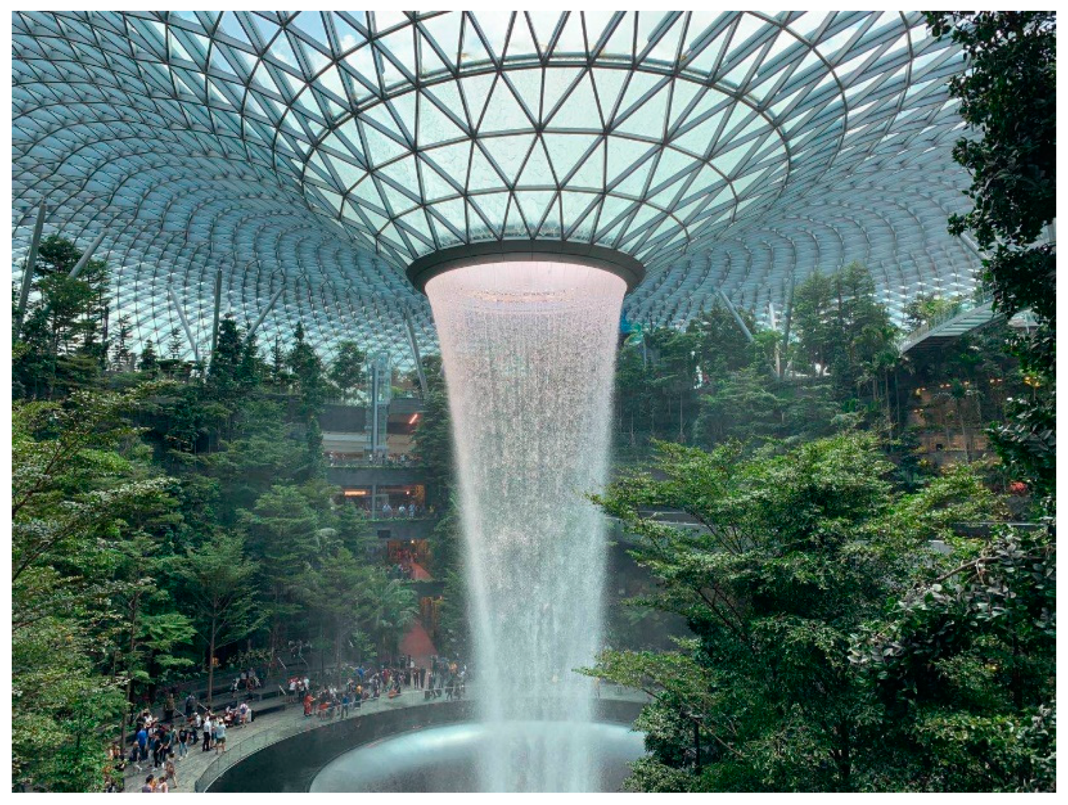
Figure 1.
Central opening of Changi airport.
Figure 1.
Central opening of Changi airport.
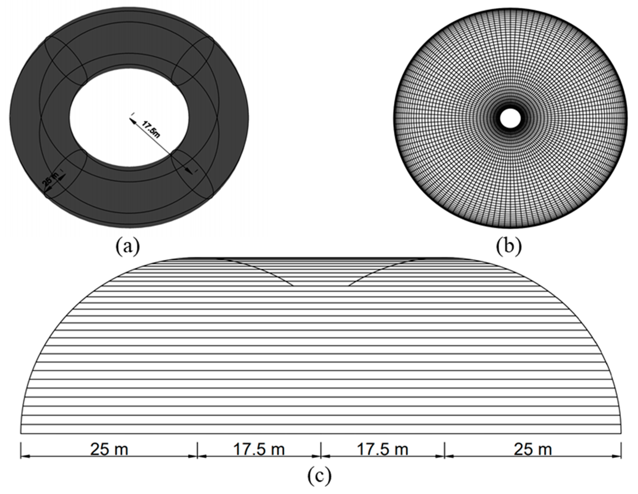
Figure 2.
Schematic design of the model ABAQUS: (a) isometric view; (b) top view; (c) front view.
Figure 2.
Schematic design of the model ABAQUS: (a) isometric view; (b) top view; (c) front view.
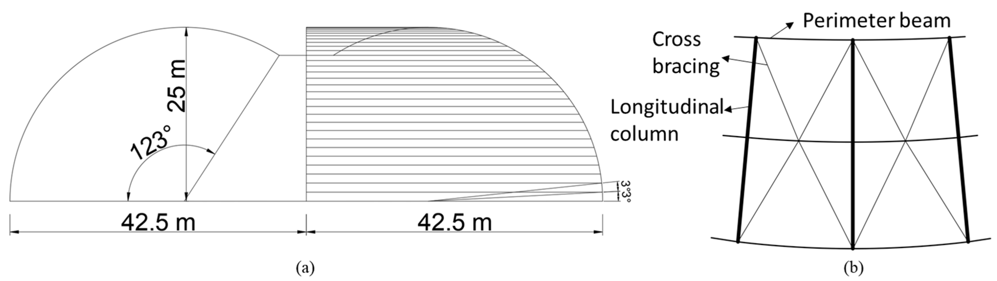
Figure 3.
Schematic design of the model: (a) front view of the half-structure; (b) structural member demonstration.
Figure 3.
Schematic design of the model: (a) front view of the half-structure; (b) structural member demonstration.
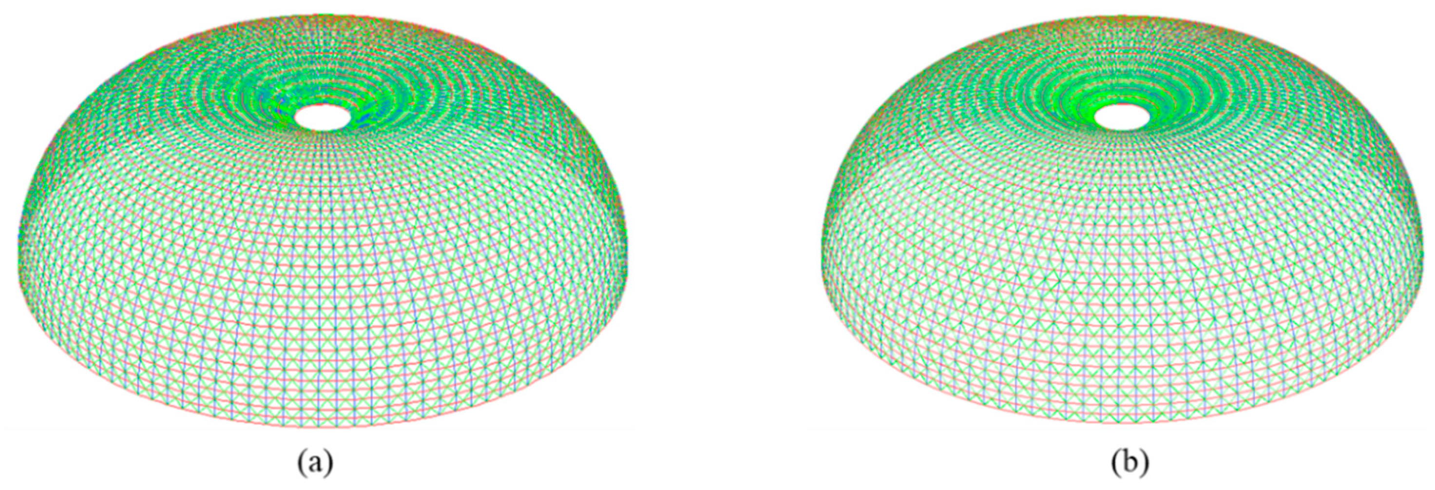
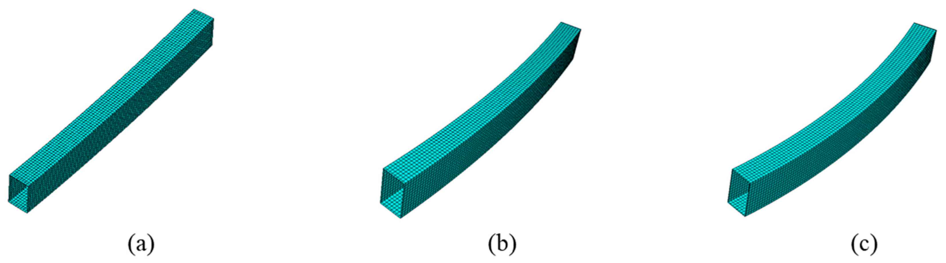
Figure 4.
Finite element models in Strand7: (a) the straight member model; (b) the curved member model.
Figure 4.
Finite element models in Strand7: (a) the straight member model; (b) the curved member model.
Figure 5.
Finite element models in ABAQUS: (a) the perimeter beam on level 5; (b) the perimeter beam on level 15; (c) the perimeter beam on level 25.
Figure 5.
Finite element models in ABAQUS: (a) the perimeter beam on level 5; (b) the perimeter beam on level 15; (c) the perimeter beam on level 25.
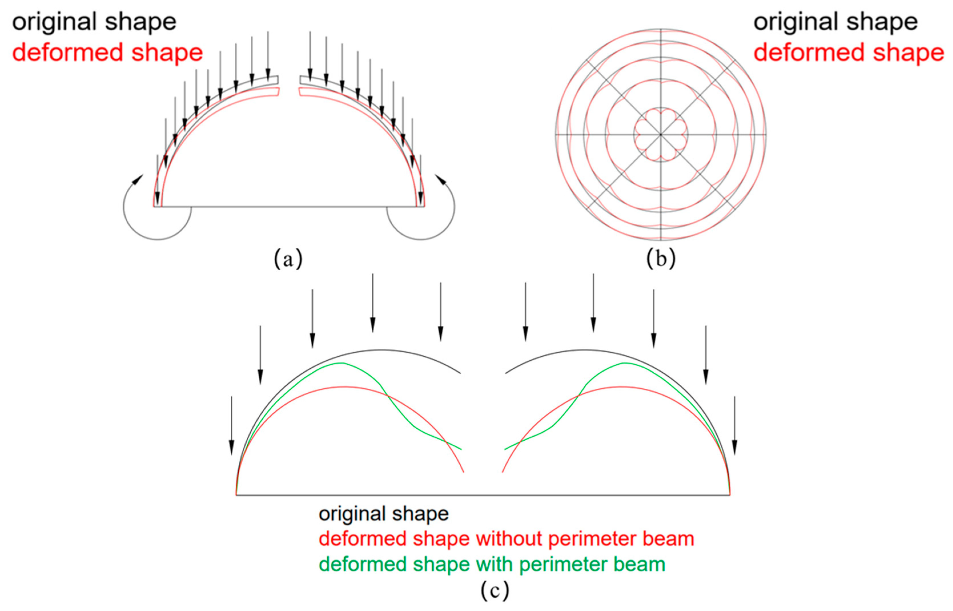
Figure 6.
The deformation of the structure under vertical loading: (a) load direction demonstration; (b) top view of deformation shape; (c) front view of deformation shape.
Figure 6.
The deformation of the structure under vertical loading: (a) load direction demonstration; (b) top view of deformation shape; (c) front view of deformation shape.
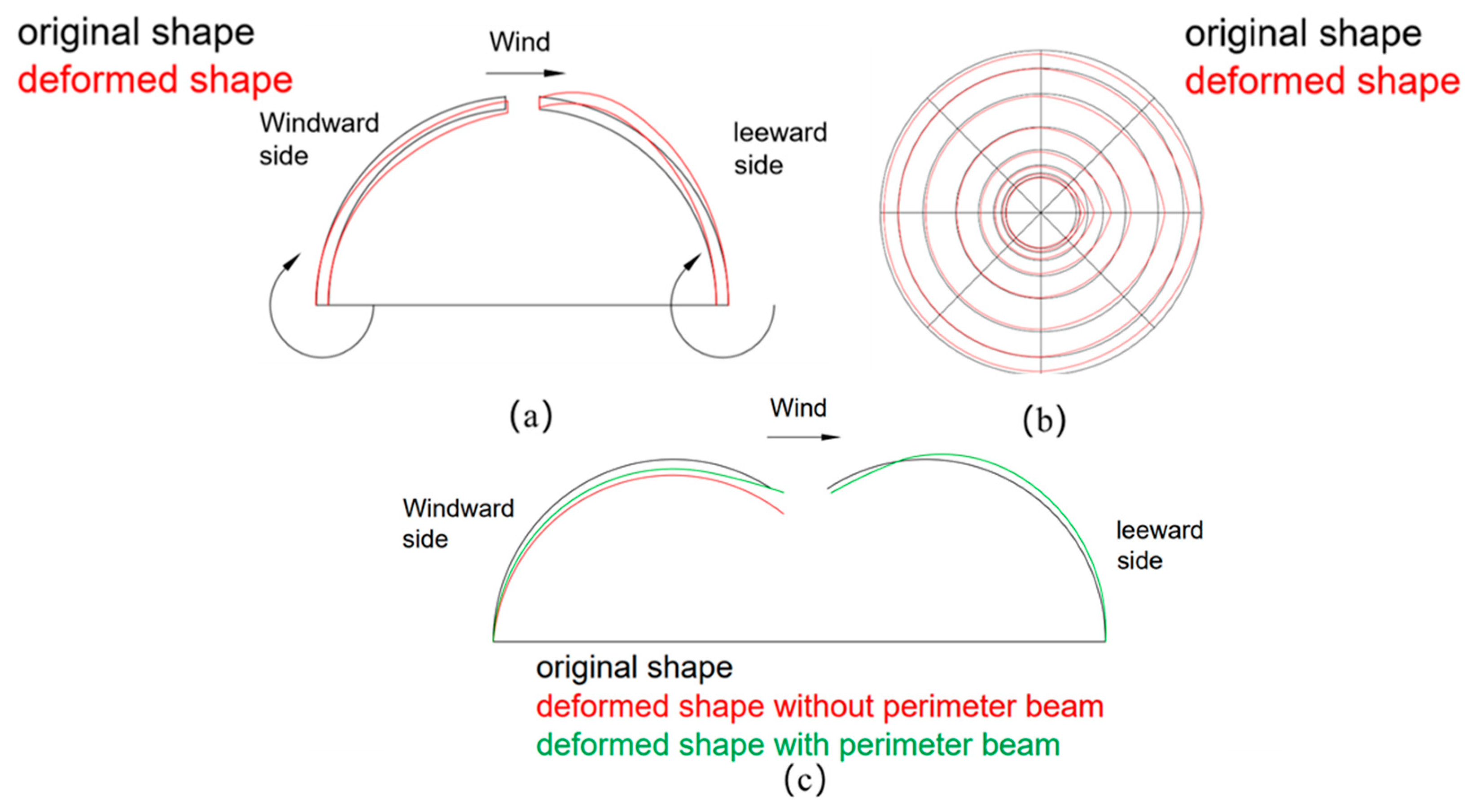
Figure 7.
The deformation of the structure under lateral loading: (a) load direction demonstration; (b) top view of deformation shape; (c) front view of deformation shape.
Figure 7.
The deformation of the structure under lateral loading: (a) load direction demonstration; (b) top view of deformation shape; (c) front view of deformation shape.
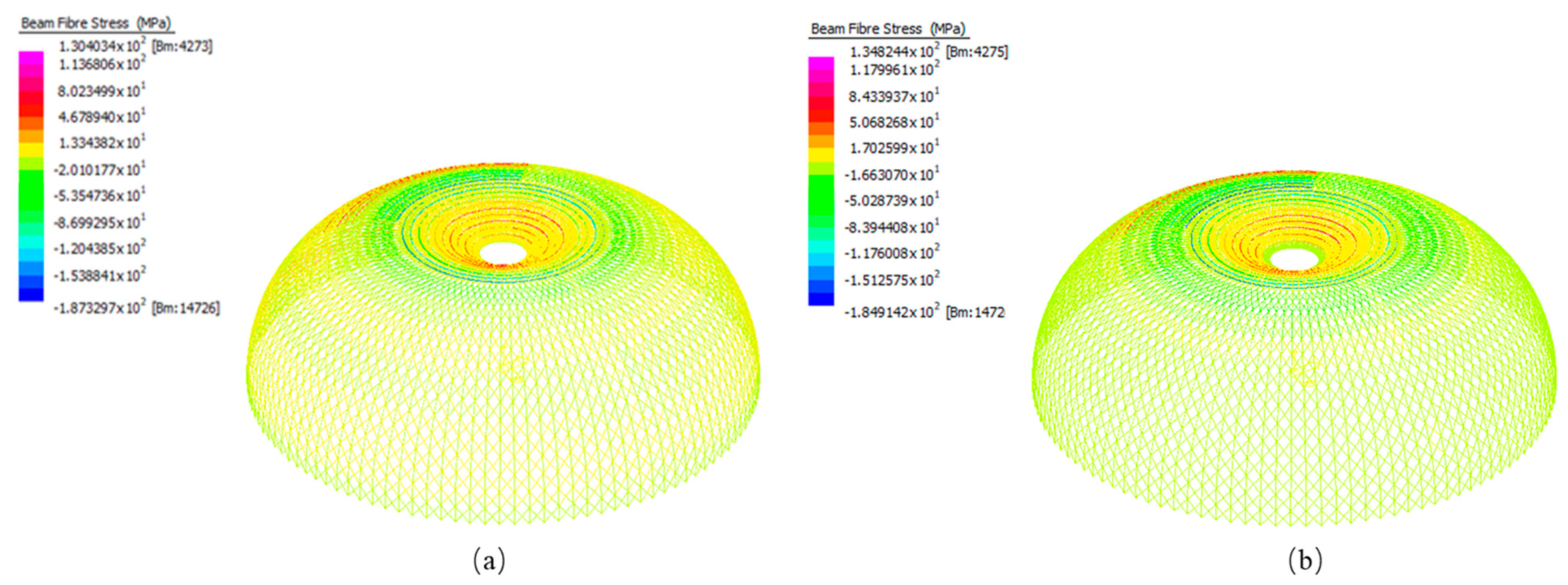
Figure 8.
(a) Linear analysis of total fiber stress of straight member model under 1.2G + 1.5Q; (b) nonlinear analysis of total fiber stress of straight member model under 1.2G + 1.5Q.
Figure 8.
(a) Linear analysis of total fiber stress of straight member model under 1.2G + 1.5Q; (b) nonlinear analysis of total fiber stress of straight member model under 1.2G + 1.5Q.
Figure 9.
(a) Linear analysis of total fiber stress of curved member model under 1.2G + 1.5Q; (b) nonlinear analysis of total fiber stress of curved member model under 1.2G + 1.5Q; (c) linear buckling analysis of the straight member model under 1.2G + 1.5Q; (d) linear buckling analysis of the curved member model under 1.2G + 1.5Q.
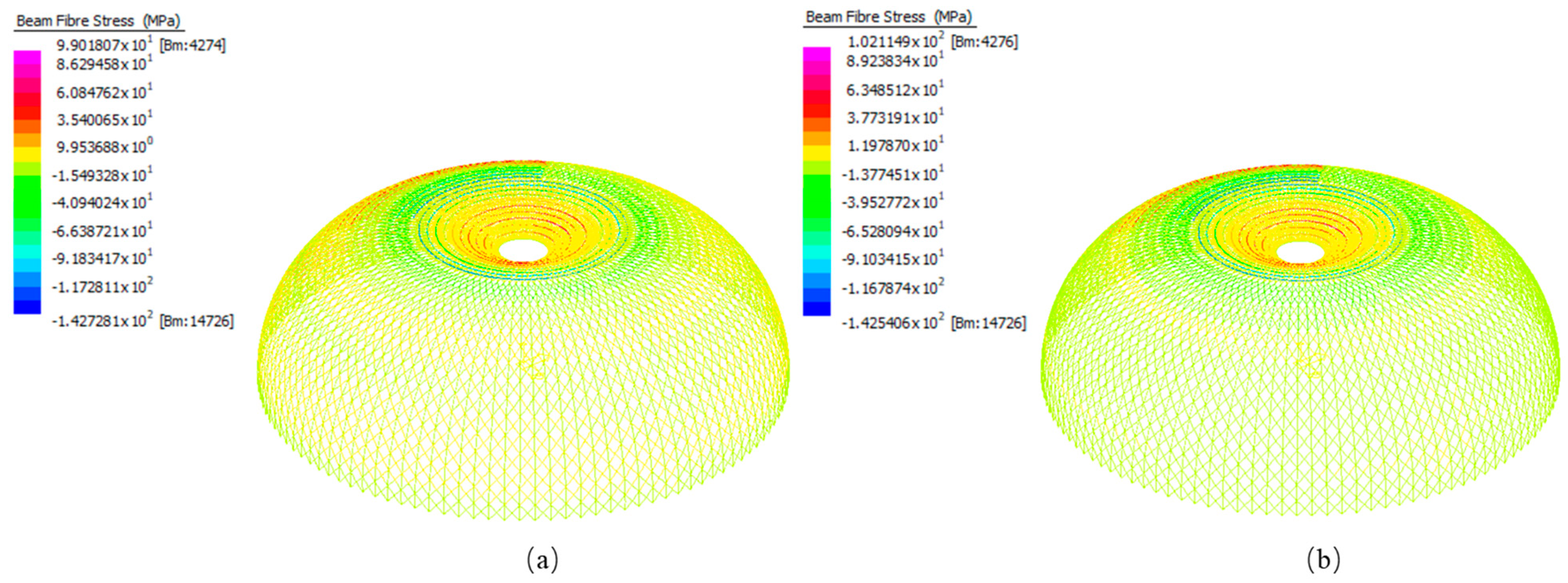
Figure 10.
(a) Linear analysis of total fiber stress of straight member model under 1.35G; (b) nonlinear analysis of total fiber stress of straight member model under 1.35G.
Figure 10.
(a) Linear analysis of total fiber stress of straight member model under 1.35G; (b) nonlinear analysis of total fiber stress of straight member model under 1.35G.
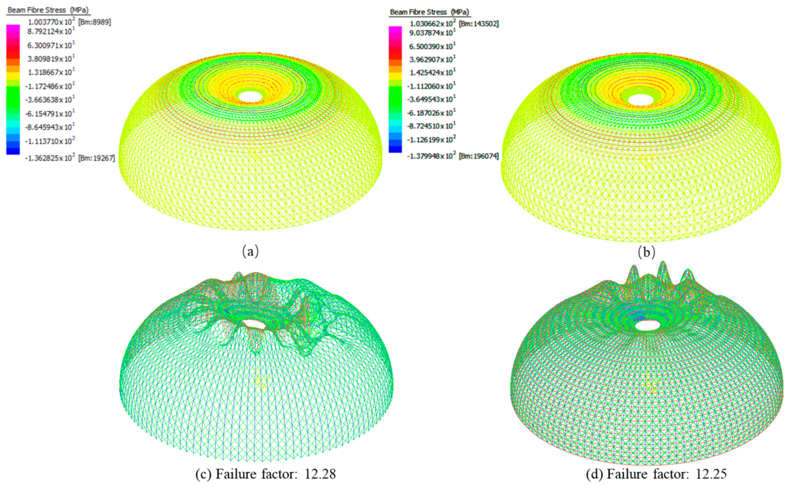
Figure 11.
(a) Linear analysis of total fiber stress of a curved member model under 1.35G; (b) nonlinear analysis of total fiber stress of a curved member model under 1.35G; (c) linear buckling analysis of the straight member model under 1.35G; (d) linear buckling analysis of the curved member model under 1.35G.
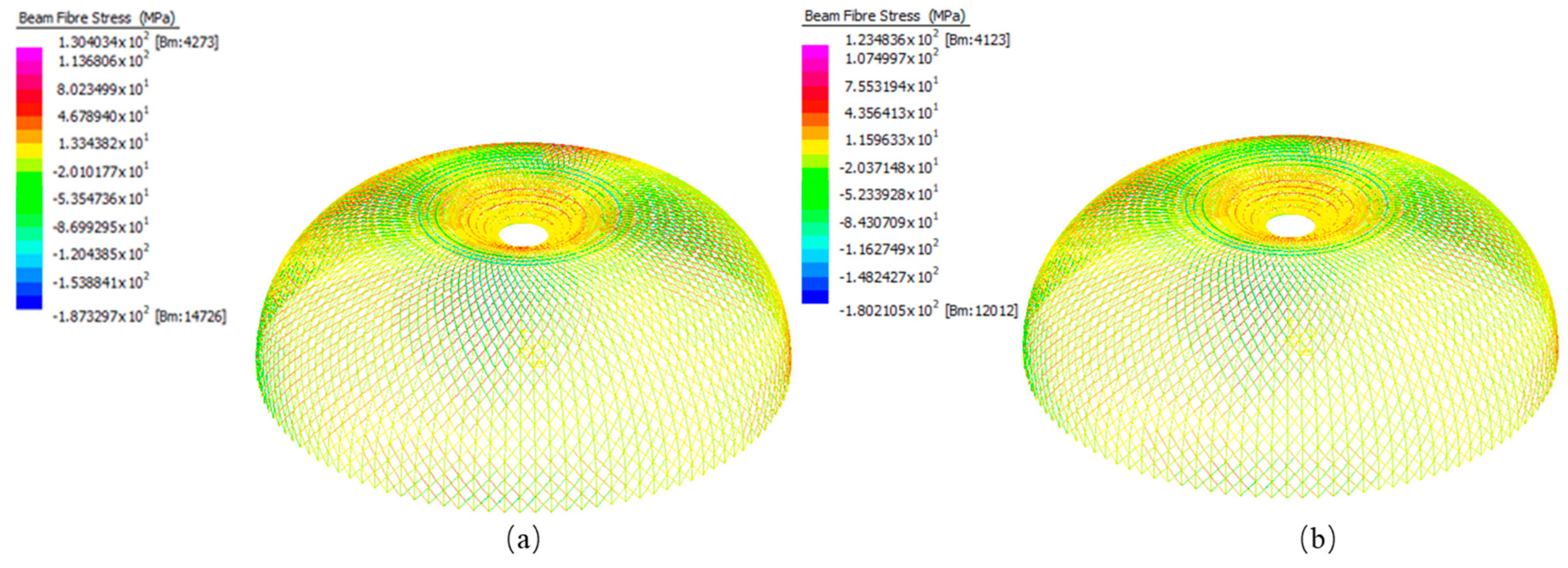
Figure 12.
(a) Linear analysis of total fiber stress of straight member model under 1.2G + W; (b) nonlinear analysis of total fiber stress of straight member model under 1.2G + W.
Figure 12.
(a) Linear analysis of total fiber stress of straight member model under 1.2G + W; (b) nonlinear analysis of total fiber stress of straight member model under 1.2G + W.
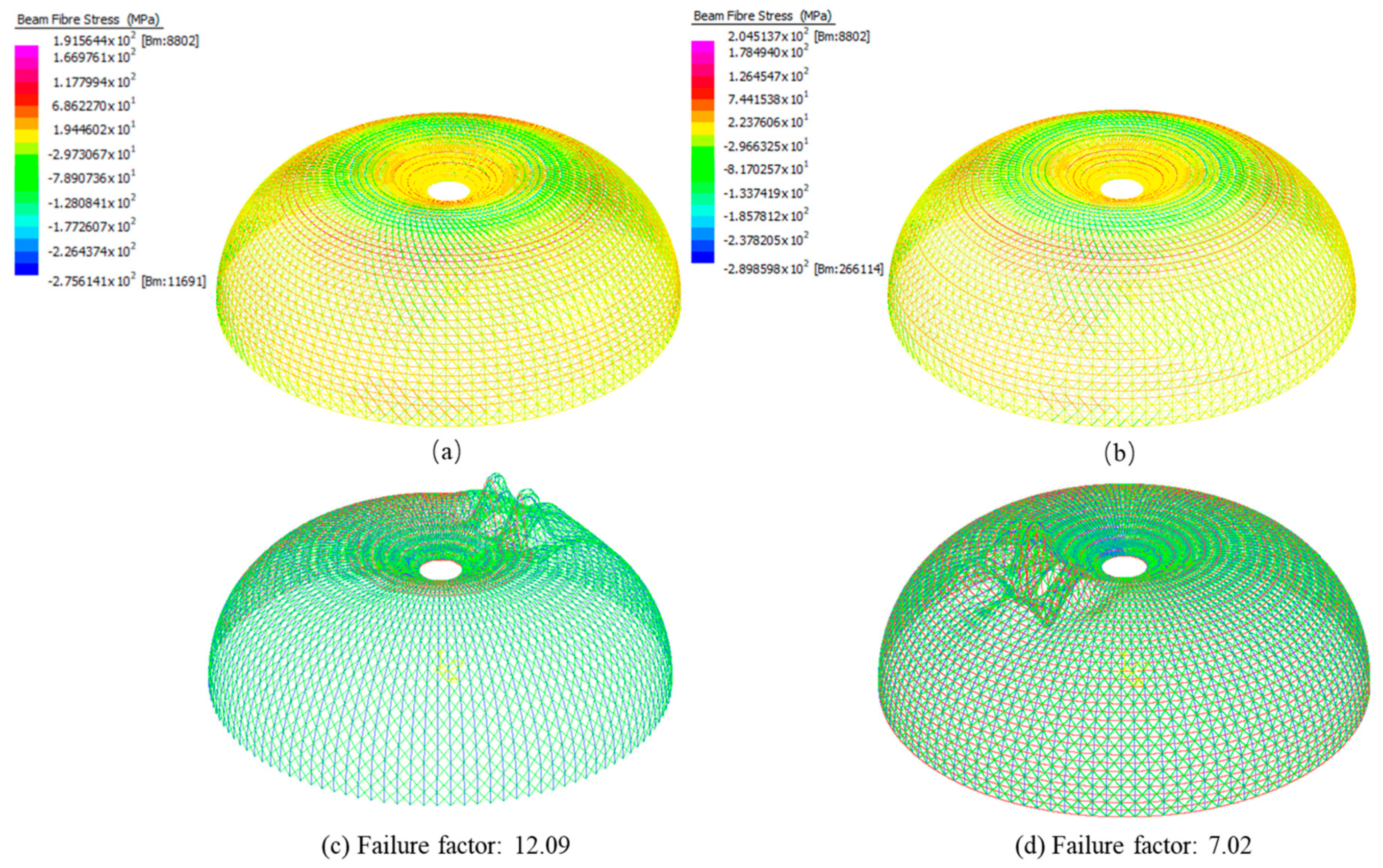
Figure 13.
(a) Linear analysis of total fiber stress of curved member model under 1.2G + W; (b) non-linear analysis of total fiber stress of curved member model under 1.2G + W; (c) linear buckling analysis of the straight member model under 1.2G + W; (d) linear buckling analysis of the curved member model under 1.2G + W.
Figure 14.
Demonstration of different loading directions for straight and curved beams: (a) the gravity load for a straight beam; (b) the gravity load for a curved beam; (c) the wind load for a straight beam; (d) the wind load for a curved beam.
Figure 14.
Demonstration of different loading directions for straight and curved beams: (a) the gravity load for a straight beam; (b) the gravity load for a curved beam; (c) the wind load for a straight beam; (d) the wind load for a curved beam.
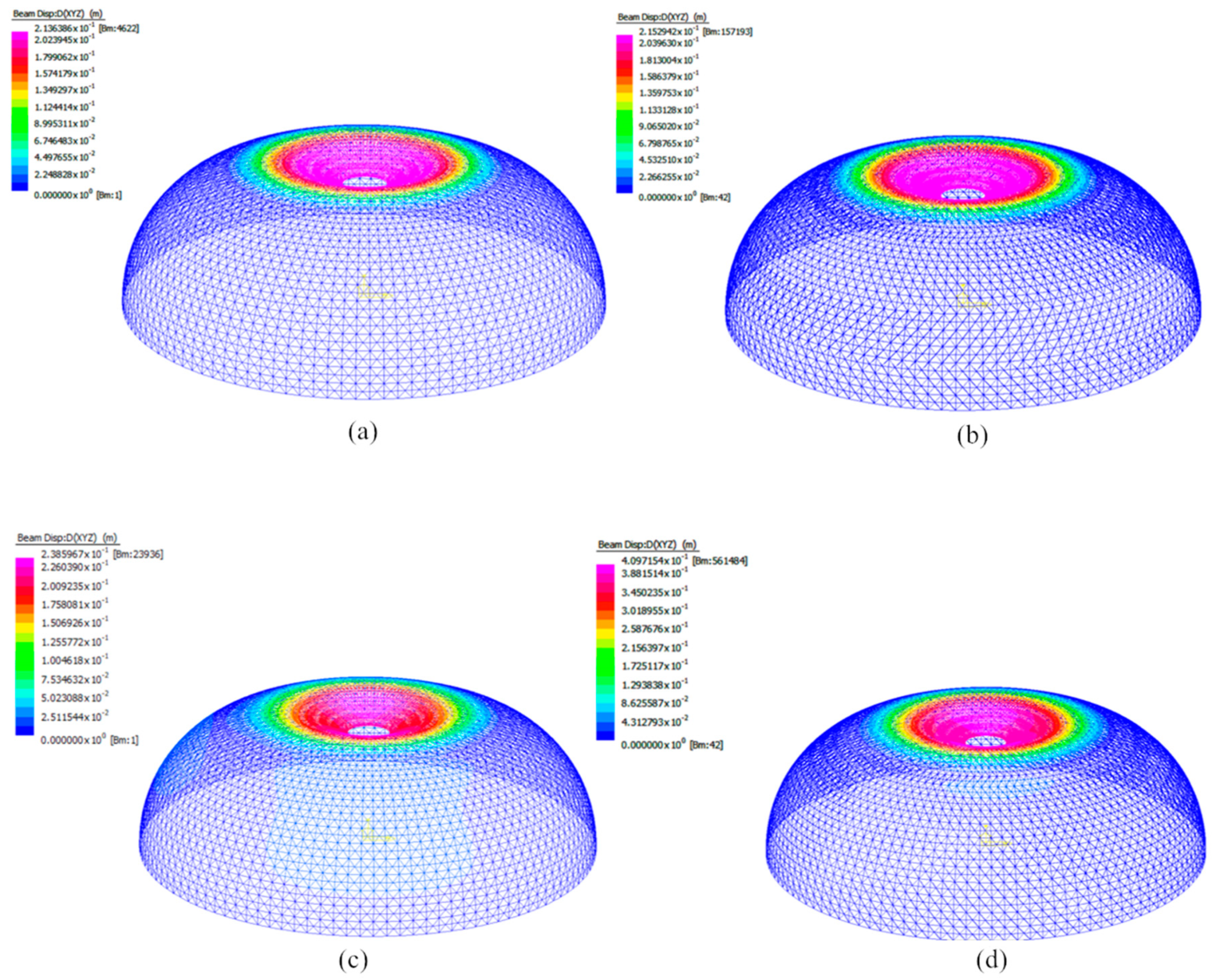
Figure 15.
(a) Total beam displacement in the straight member model by linear static analysis (G + 0.7Q); (b) total beam displacement in the curved member model by linear static analysis (G + 0.7Q); (c) total beam displacement in the straight member model by linear static analysis (G + 0.7Q + W); (d) total beam displacement in the curved member model by linear static analysis (G + 0.7Q + W).
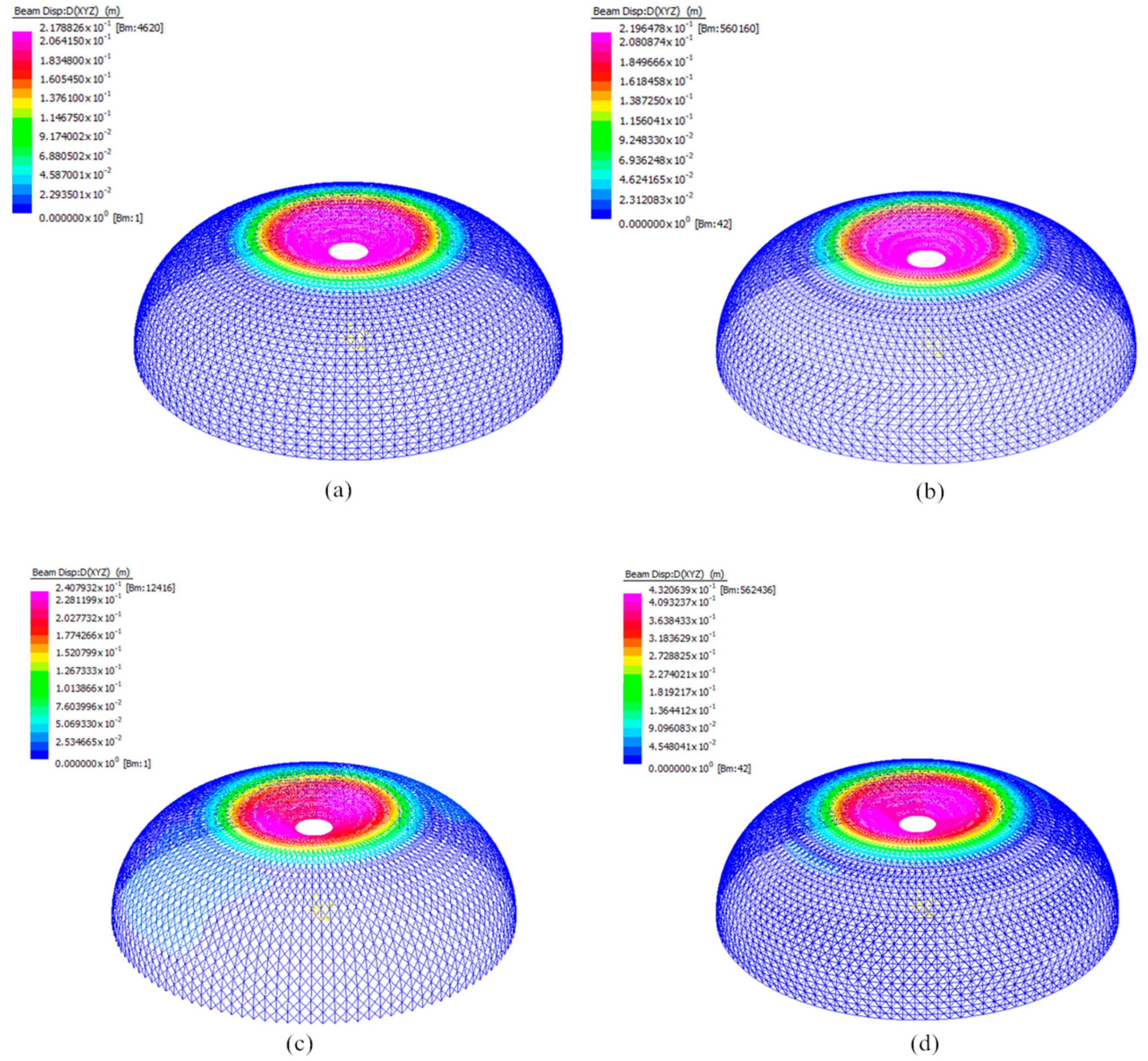
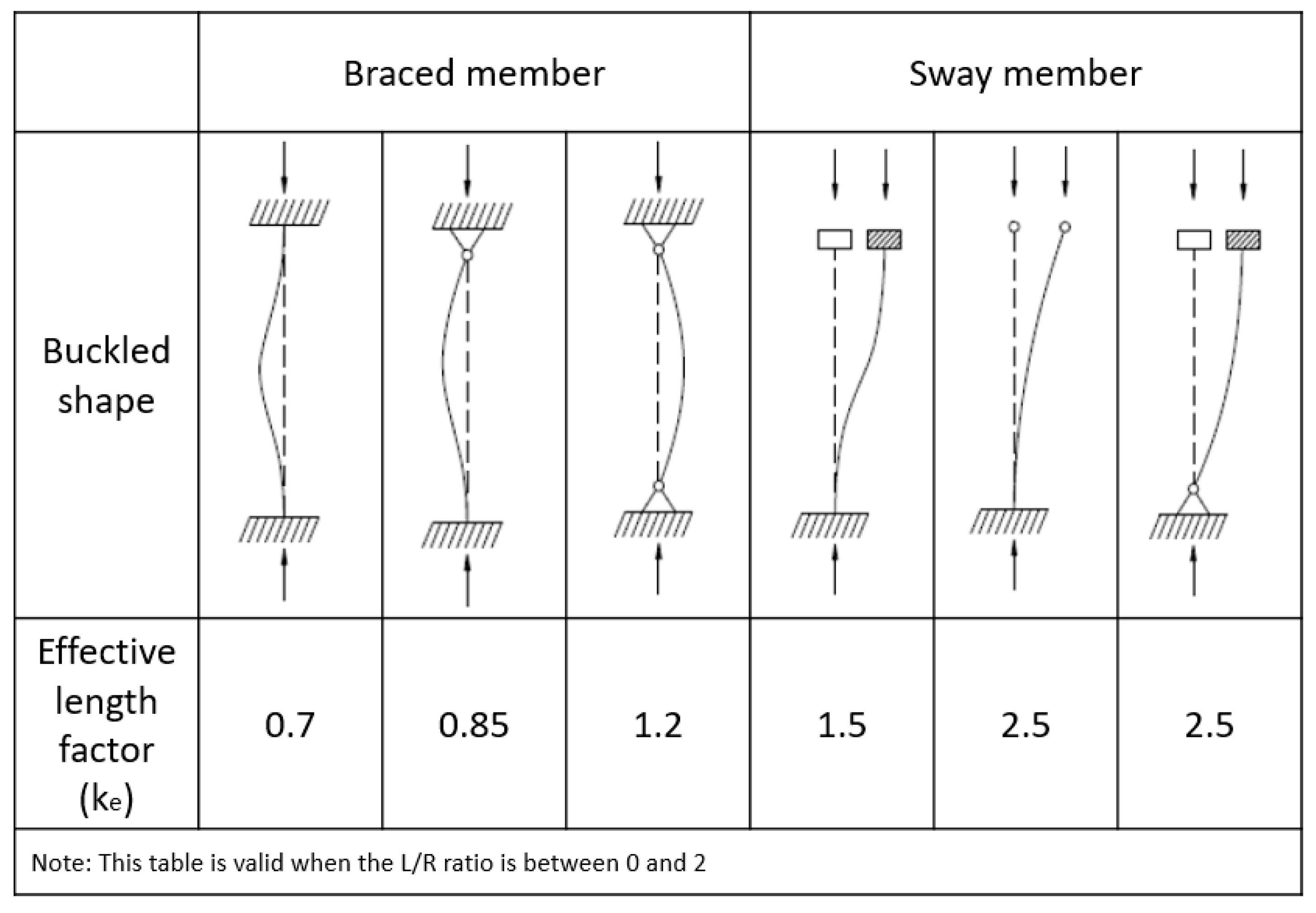
Figure 17.
The effective length factor provided by AS4100.
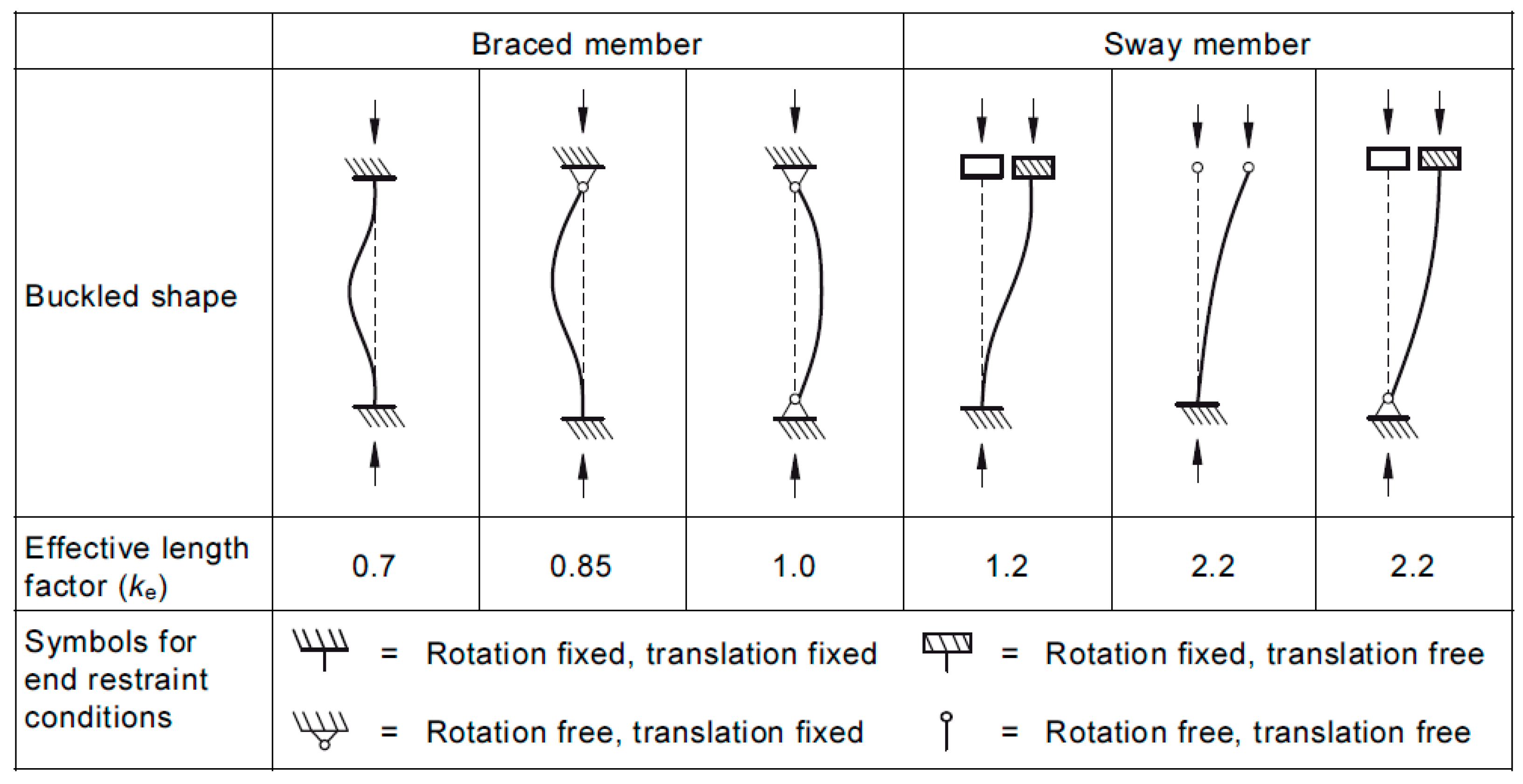
Figure 17.
The effective length factor provided by AS4100.
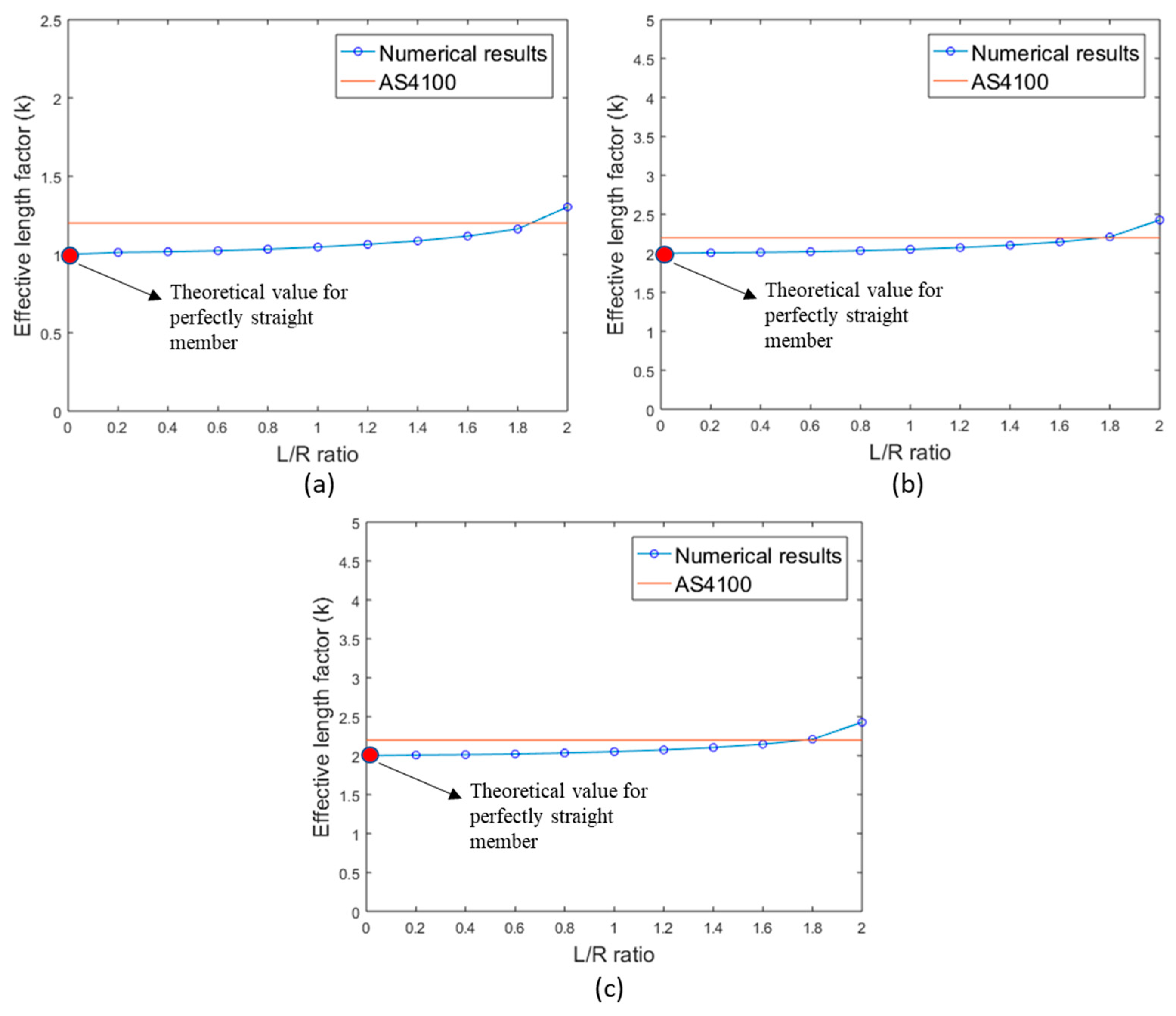
Figure 18.
The effective length factor () of curved columns under different L/R ratios: (a) braced member case 1; (b) braced member case 2; (c) braced member case 3.
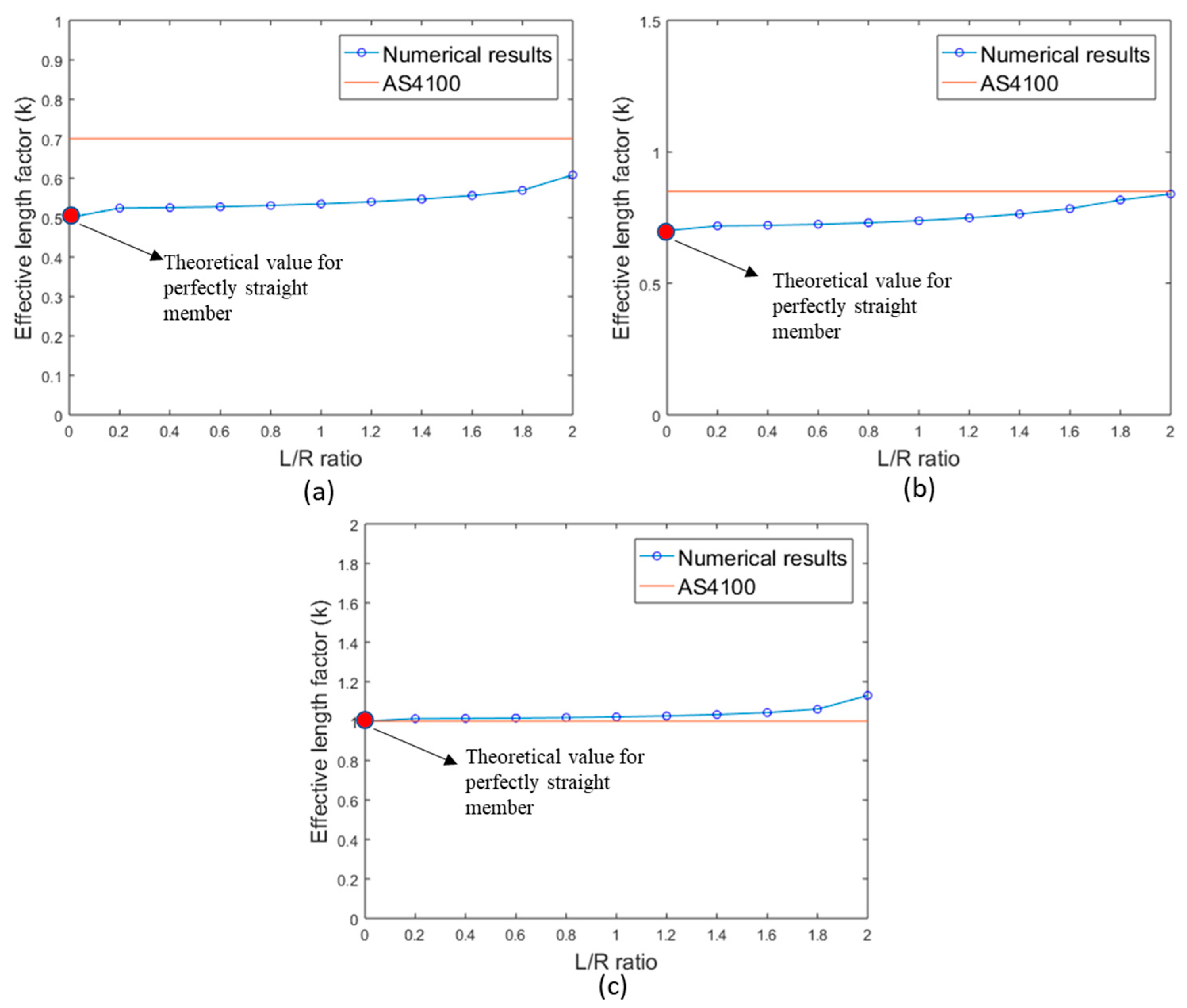
Figure 18.
The effective length factor () of curved columns under different L/R ratios: (a) braced member case 1; (b) braced member case 2; (c) braced member case 3.
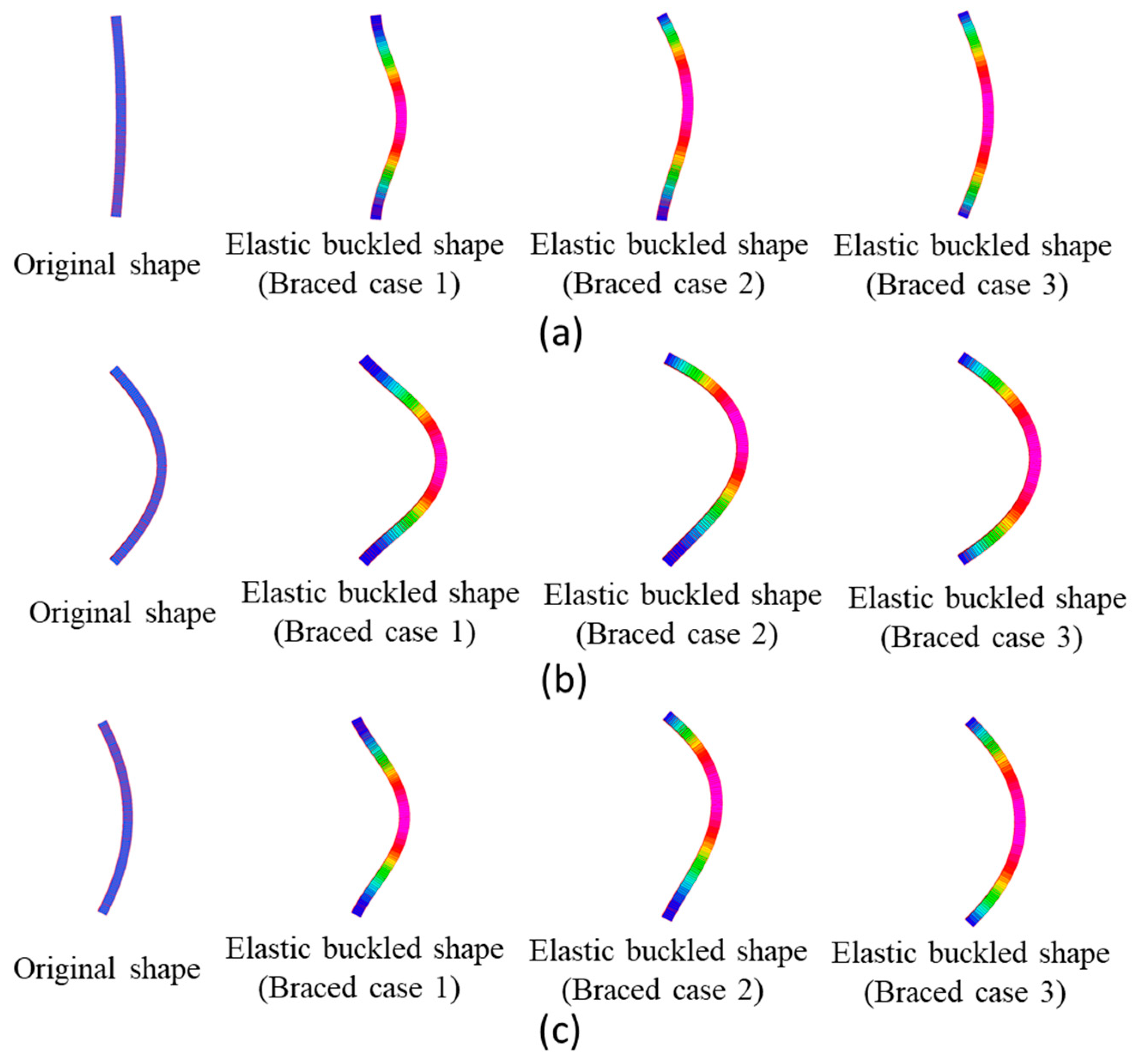
Figure 19.
(a) The critical elastic buckled shape for the curved column with L/R ratio 0.4; (b) the critical elastic buckled shape for the curved column with L/R ratio 1.0; (c) the critical elastic buckled shape for the curved column with L/R ratio 1.8.
Figure 19.
(a) The critical elastic buckled shape for the curved column with L/R ratio 0.4; (b) the critical elastic buckled shape for the curved column with L/R ratio 1.0; (c) the critical elastic buckled shape for the curved column with L/R ratio 1.8.
Figure 20.
The effective length factor (ke) of curved beams under different L/R ratios: (a) sway member case 1; (b) sway member case 2; (c) sway member case 3.
Figure 20.
The effective length factor (ke) of curved beams under different L/R ratios: (a) sway member case 1; (b) sway member case 2; (c) sway member case 3.
Figure 21.
(a) The critical elastic buckled shape for the curved column with L/R ratio 0.4; (b) the critical elastic buckled shape for the curved column with L/R ratio 1.0; (c) the critical elastic buckled shape for the curved column with L/R ratio 1.8.
Figure 21.
(a) The critical elastic buckled shape for the curved column with L/R ratio 0.4; (b) the critical elastic buckled shape for the curved column with L/R ratio 1.0; (c) the critical elastic buckled shape for the curved column with L/R ratio 1.8.
Figure 22.
The proposed effective length factor for curved members.
Figure 22.
The proposed effective length factor for curved members.
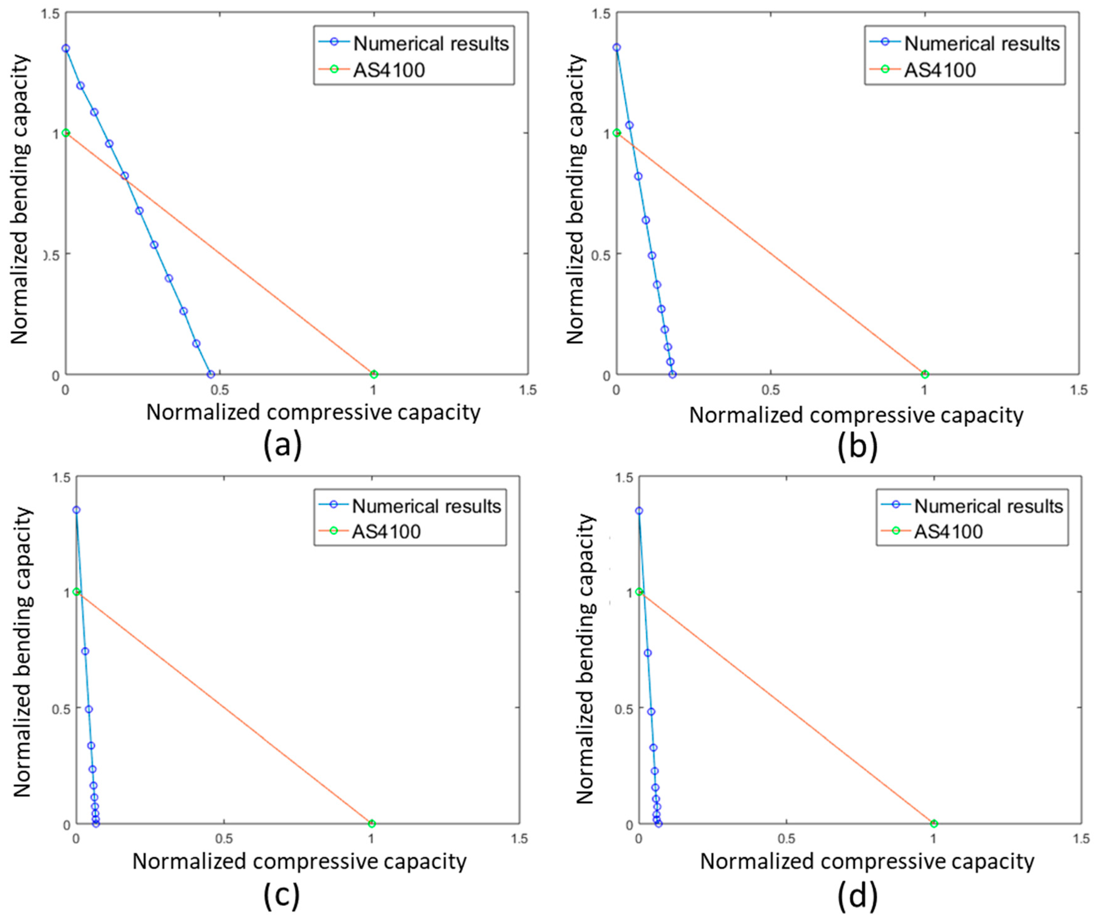
Figure 23.
Interaction curves of the members with different L/R ratios: (a) for 0.4 L/R ratio; (b) for 0.8 L/R ratio; (c) for 1.2 L/R ratio; (d) for 1.8 L/R ratio.
Figure 23.
Interaction curves of the members with different L/R ratios: (a) for 0.4 L/R ratio; (b) for 0.8 L/R ratio; (c) for 1.2 L/R ratio; (d) for 1.8 L/R ratio.
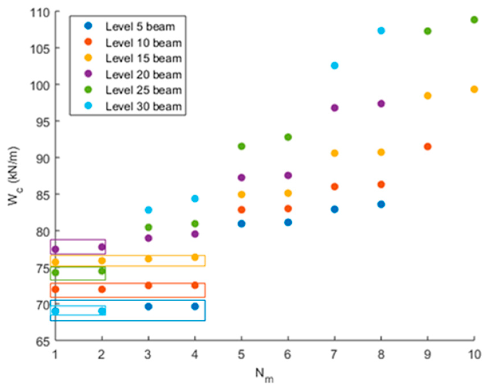
Figure 24.
The elastic buckling loads (Wc) of different modes (Nm) for the curved beams on different levels.
Figure 24.
The elastic buckling loads (Wc) of different modes (Nm) for the curved beams on different levels.
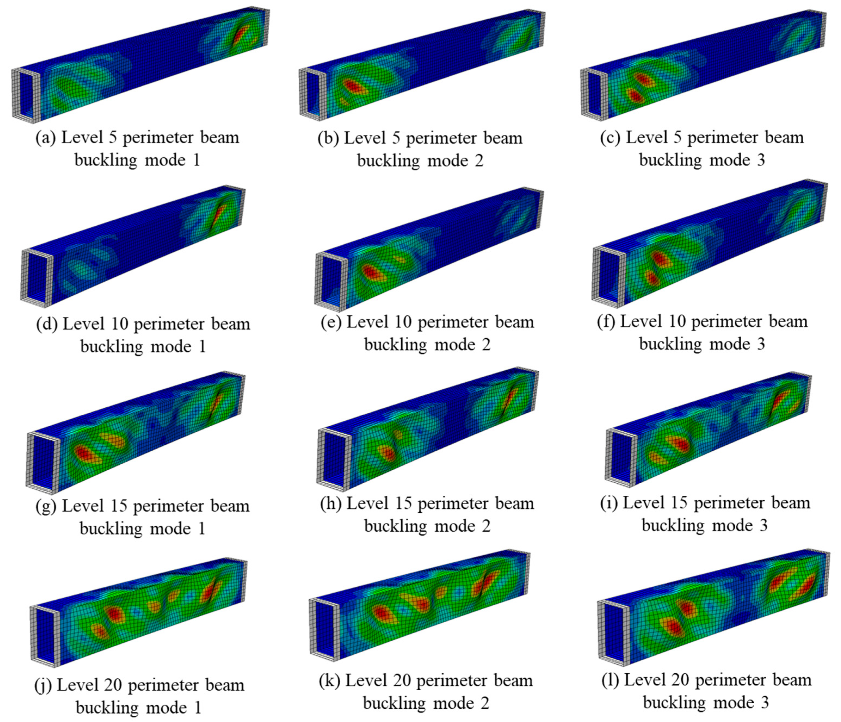
Figure 25.
The buckling shapes of different modes of each curved beam.
Figure 25.
The buckling shapes of different modes of each curved beam.
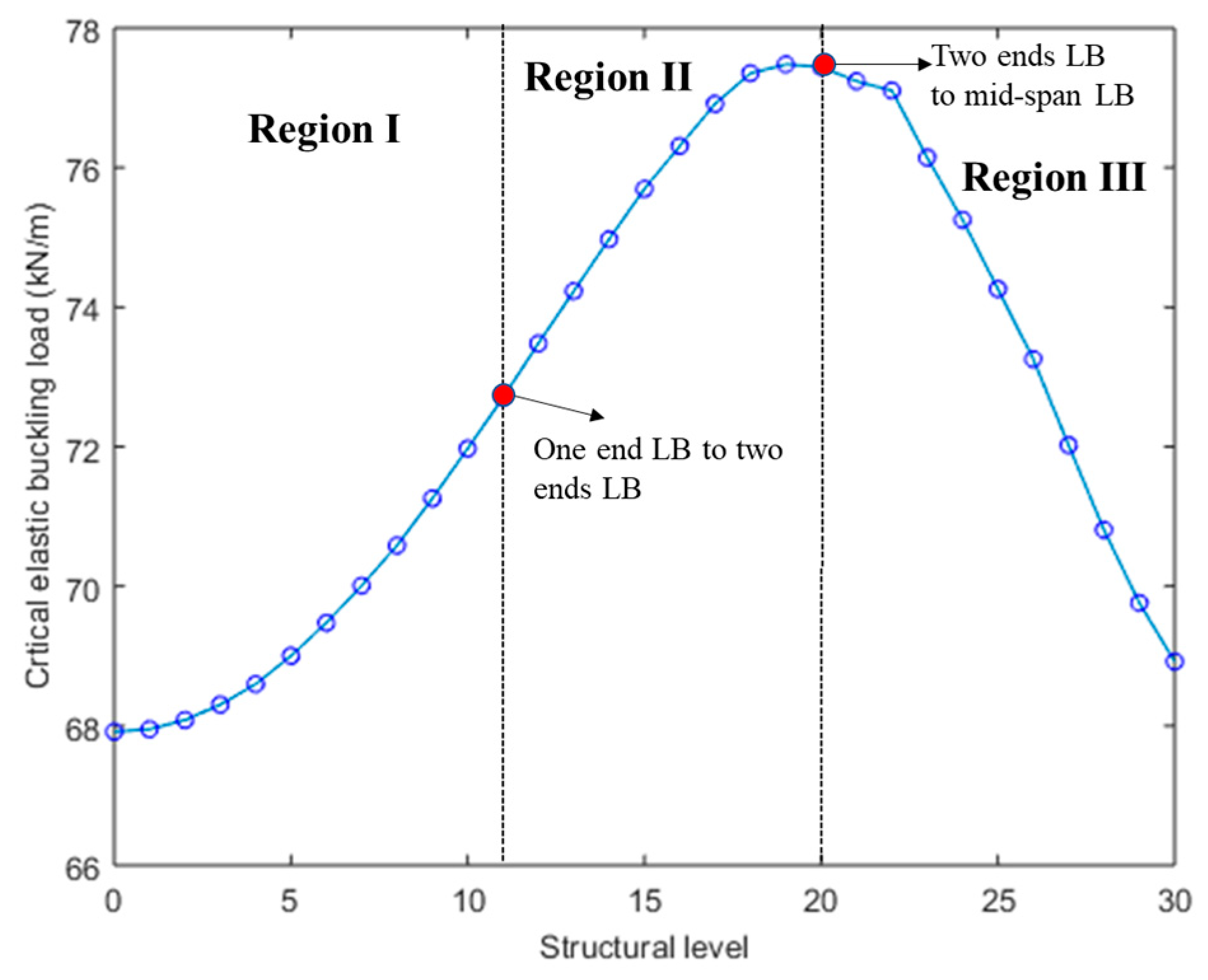
Figure 26.
The elastic buckling loads (Wc) of different structural level (SL) perimeter beams.
Figure 26.
The elastic buckling loads (Wc) of different structural level (SL) perimeter beams.
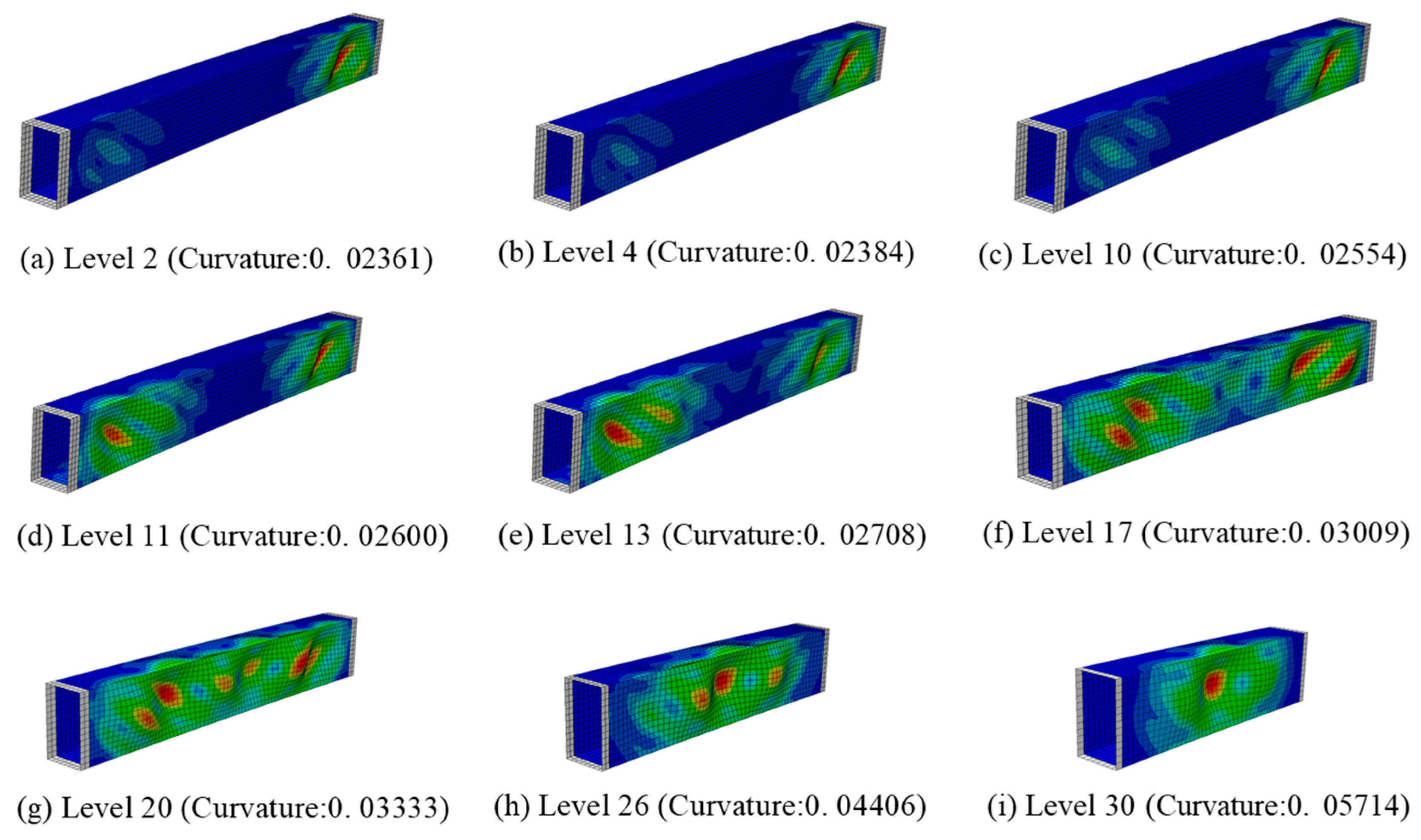
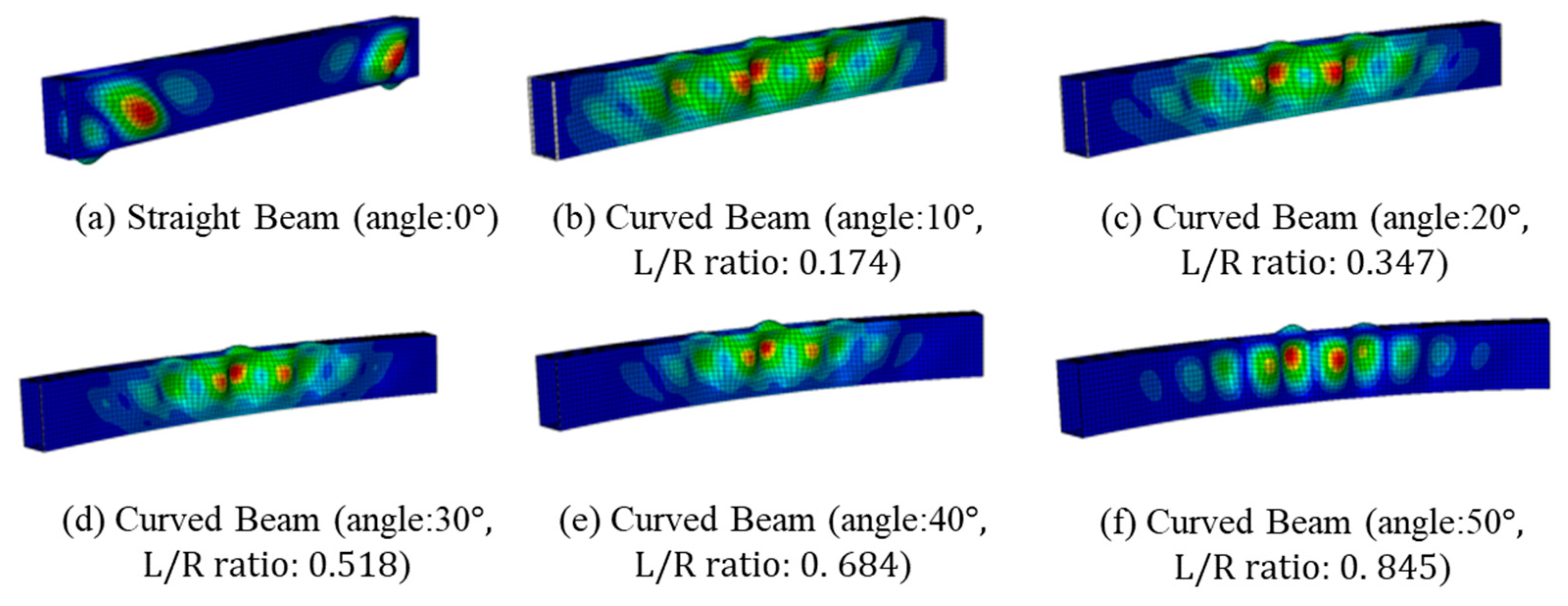
Figure 27.
The buckling shapes for the perimeter beams with different curvature.
Figure 27.
The buckling shapes for the perimeter beams with different curvature.
Figure 28.
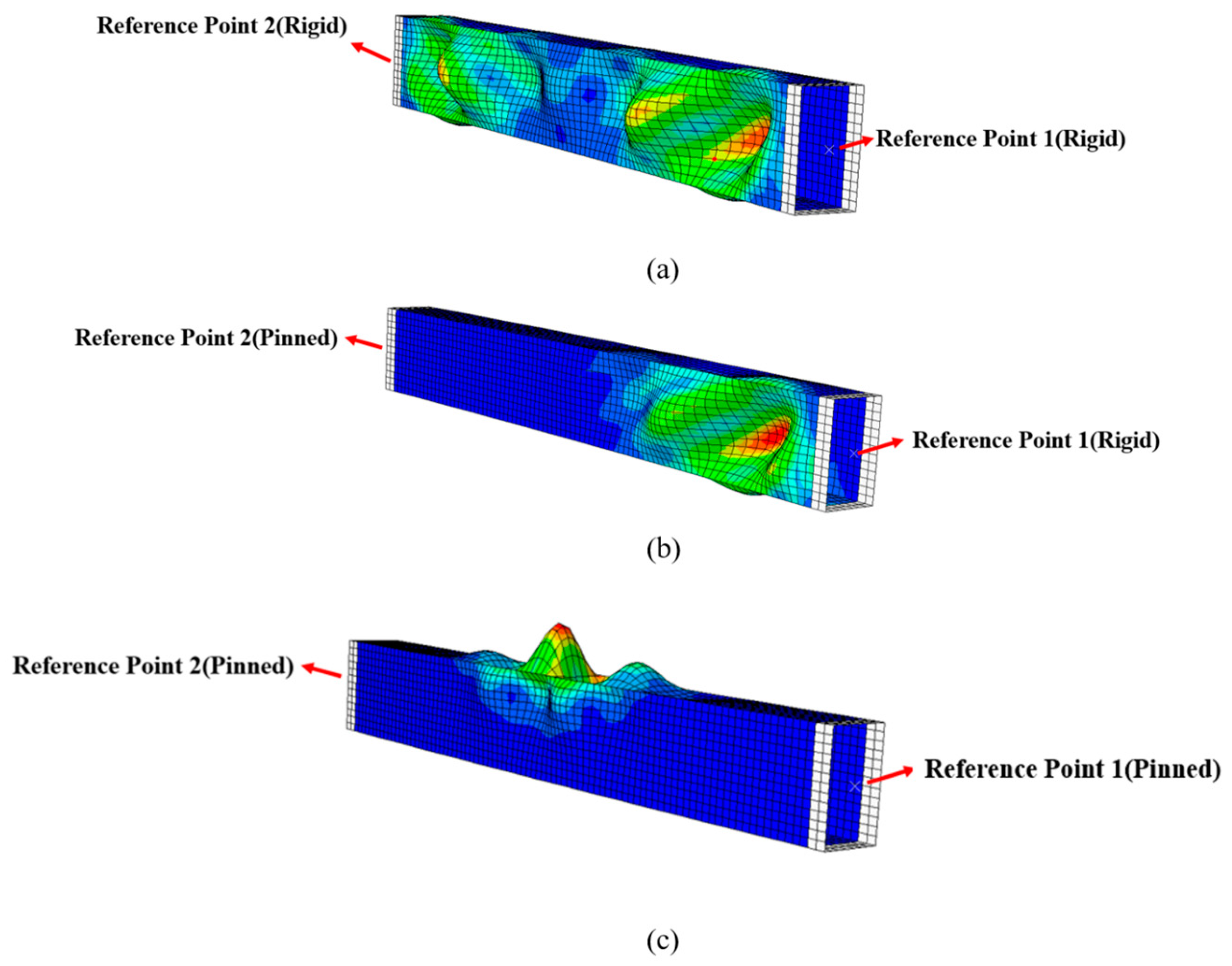
(a) Buckling mode of the rigid–rigid perimeter beam; (b) buckling mode of the rigid–pinned perimeter beam; (c) buckling mode of the pinned–pinned perimeter beam.
Figure 28.
(a) Buckling mode of the rigid–rigid perimeter beam; (b) buckling mode of the rigid–pinned perimeter beam; (c) buckling mode of the pinned–pinned perimeter beam.
Figure 29.
Buckling shape of some selected beams.
Figure 29.
Buckling shape of some selected beams.
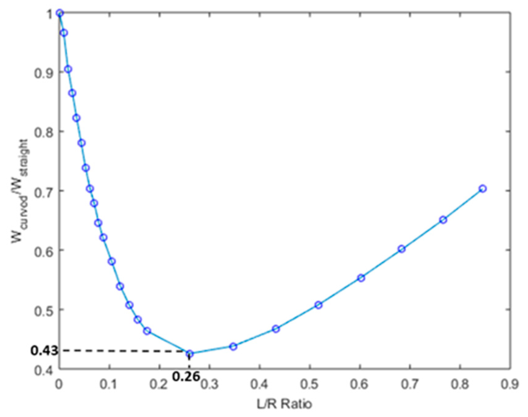
Figure 30.
The buckling capacity ratio of curved members with different L/R ratios.
Figure 30.
The buckling capacity ratio of curved members with different L/R ratios.
Table 1.
Section property for different members.
Table 1.
Section property for different members.
| | Perimeter Beams | Cross Bracing | Longitudinal Columns |
|---|
| Section name | 250 × 150 × 9 RHS | 101.6 × 3.2 CHS | 250 × 250 × 9 RHS |
| Yield stress (MPa) | 350 | 350 | 350 |
| Section area (mm2) | 6600 | 989.2 | 8400 |
| Second moment area (x-axis) (mm4) | 5.37 × 10⁷ | 1.199 × 10⁶ | 7.98 × 10⁷ |
| Second moment area (y-axis) (mm4) | 2.43 × 10⁷ | 1.199 × 10⁶ | 7.98 × 10⁷ |
Table 2.
Wind loads on the structure.
Table 2.
Wind loads on the structure.
| Region | Windward Quarter | Sides | Leeward Quarter |
|---|
| Pressure (kPa) | +2.44 | −4.82 | −0.19 |
| UDL (kN/m) | 1.83 | −3.615 | −0.143 |
Table 3.
The linear load combinations.
Table 3.
The linear load combinations.
| | Strength Limit State | Serviceability Limit State |
|---|
| Load combinations | 1.2G + 1.5Q | G + 0.7Q |
| 1.35G | G + 0.7Q + W |
| 1.2G + W | |
Table 4.
Fiber stresses under 1.2G + 1.5Q.
Table 4.
Fiber stresses under 1.2G + 1.5Q.
| Solver | Straight Member Model | Curved Member Model | Difference |
|---|
| Maximum Fiber Stress (MPa) | Critical Member | Maximum Fiber Stress (MPa) | Critical Member |
|---|
| Linear static | 130.40 | Longitudinal columns on the top ring | 132.23 | Longitudinal columns on the top ring | 1.38% |
| Nonlinear static | 134.82 | Longitudinal columns on the top ring | 136.06 | Longitudinal columns on the top ring | 0.96% |
Nonlinear static
Load increments | 2.4 | Nonlinear static
Load increments | 2.2 |
Table 5.
Displacements under 1.2G + 1.5Q.
Table 5.
Displacements under 1.2G + 1.5Q.
| Solver | Straight Member Model Maximum Displacements (mm) |
| Dx | Dy | Dz | Dxyz |
| Linear static | −13.8 | −13.0 | −299 | 299 |
| Nonlinear static | −14.1 | 13.3 | −309 | 230 |
| Solver | Curved Member Model Maximum Displacements (mm) |
| Dx | Dy | Dz | Dxyz |
| Linear static | −13.1 | 13.1 | −301 | 301 |
| Nonlinear static | −13.5 | 13.5 | −312 | 312 |
Table 6.
Fiber stresses under 1.35G.
Table 6.
Fiber stresses under 1.35G.
| Solver | Straight Member Model | Curved Member Model | Difference |
|---|
| Maximum Fiber Stress (MPa) | Critical Member | Maximum Fiber Stress (MPa) | Critical Member | |
|---|
| Linear static | 99.02 | Longitudinal columns on the top ring | 100.38 | Longitudinal columns on the top ring | 1.37% |
| Nonlinear static | 102.11 | Longitudinal columns on the top ring | 103.07 | Longitudinal columns on the top ring | 0.94% |
Nonlinear static
Load increments | 3.1 | Nonlinear static
Load increments | 2.7 |
Table 7.
Displacements under 1.35G.
Table 7.
Displacements under 1.35G.
| Solver | Straight Member Model Maximum Displacements (mm) |
| Dx | Dy | Dz | Dxyz |
| Linear static | −10.6 | 99.1 | −227 | 227 |
| Nonlinear static | −10.8 | 10.2 | −234 | 234 |
| Solver | Curved Member Model Maximum Displacements (mm) |
| Dx | Dy | Dz | Dxyz |
| Linear static | 9.99 | −9.99 | −229 | 229 |
| Nonlinear static | 10.3 | 10.3 | −236 | 236 |
Table 8.
Fiber stresses under 1.2G + W.
Table 8.
Fiber stresses under 1.2G + W.
| Solver | Straight Member Model | Curved Member Model | Difference |
|---|
| Maximum Fiber Stress (MPa) | Critical Member | Maximum Fiber Stress (MPa) | Critical Member |
|---|
| Linear static | 117.27 | Longitudinal columns on the top ring | 191.56 | Longitudinal columns on the top ring | 63.34% |
| Nonlinear static | 123.48 | Longitudinal columns on the top ring | 204.51 | Longitudinal columns on the top ring | 65.62% |
Nonlinear static
load increments | 3.3 | Nonlinear static
load increments | 1.6 |
Table 9.
Displacements under 1.2G + W.
Table 9.
Displacements under 1.2G + W.
| Solver | Straight Member Model Maximum Displacements (mm) |
| Dx | Dy | Dz | Dxyz |
| Linear static | 23.7 | −17.9 | −227 | 227 |
| Nonlinear static | 22.6 | −16.8 | −230 | 230 |
| Solver | Curved Member Model Maximum Displacements (mm) |
| Dx | Dy | Dz | Dxyz |
| Linear static | 31.5 | 21.8 | −420 | 420 |
| Nonlinear static | 31.5 | 21.9 | −398 | 398 |
Table 10.
Maximum structural displacement under serviceability limit state (linear static analysis).
Table 10.
Maximum structural displacement under serviceability limit state (linear static analysis).
| The Straight Member Model |
| Load Combination | Dx (mm) | Dy (mm) | Dz (mm) | Dxy (mm) | Dxyz (mm) |
| G + 0.7Q | −9.89 | 9.30 | −213.63 | 9.90 | 213.64 |
| G + 0.7Q + W | 24.19 | −18.20 | −238.23 | 24.19 | 238.60 |
| The Curved Member Model |
| Load Combination | Dx (mm) | Dy (mm) | Dz (mm) | Dxy (mm) | Dxyz (mm) |
| G + 0.7Q | −9.373 | 9.373 | −215.28 | 9.373 | 215.29 |
| G + 0.7Q + W | 32.00 | 22.09 | −409.44 | 32.00 | 409.72 |
Table 11.
Maximum structural displacement under serviceability limit state (non-linear static analysis).
Table 11.
Maximum structural displacement under serviceability limit state (non-linear static analysis).
| | The Straight Member Model Using Straight Beam Elements |
| Load Combination | Dx (mm) | Dy (mm) | Dz (mm) | Dxy (mm) | Dxyz (mm) |
| G + 0.7Q | −10.01 | 9.44 | 217.83 | 10.02 | 217.84 |
| G + 0.7Q + W | 23.07 | −17.15 | −240.50 | 23.07 | 240.79 |
| | The Curved Member Model Using Curved Beam Elements |
| Load Combination | Dx (mm) | Dy (mm) | Dz (mm) | Dxy (mm) | Dxyz (mm) |
| G + 0.7Q | 9.56 | 9.56 | 219.64 | 9.56 | 219.65 |
| G + 0.7Q + W | 32.01 | 22.23 | −432.84 | 32.02 | 432.06 |
Table 12.
Maximum axial stress on each type of structural component (Non-linear static analysis).
Table 12.
Maximum axial stress on each type of structural component (Non-linear static analysis).
| The Straight Member Model Using Straight Beam Elements |
| Load Combination | Solver | Axial Stress (MPa) |
| G + 0.7Q | Linear static | 52.75 |
| G + 0.7Q | Non-linear static | 53.14 |
| G + 0.7Q + W | Linear static | 81.03 |
| G + 0.7Q + W | Non-linear static | 77.76 |
| The Curved Member Model Using Curved Beam Elements |
| Load Combination | Solver | Axial Stress (MPa) |
| G + 0.7Q | Linear static | 51.62 |
| G + 0.7Q | Non-linear static | 51.89 |
| G + 0.7Q + W | Linear static | 103.04 |
| G + 0.7Q + W | Non-linear static | 107.57 |
Table 13.
The elastic buckling loads for braced longitudinal columns.
Table 13.
The elastic buckling loads for braced longitudinal columns.
| L/R Ratio | Elastic Buckling Load (kN) |
|---|
| Brace Member Case 1 | Brace Member Case 2 | Brace Member Case 3 |
|---|
| 0 | 5858.9 | 3117.89 | 1567.75 |
| 0.2 | 5849.19 | 3111.3 | 1566.79 |
| 0.4 | 5819.14 | 3090.88 | 1563.87 |
| 0.6 | 5774.62 | 3058.29 | 1558.75 |
| 0.8 | 5703.19 | 3009.69 | 1550.89 |
| 1 | 5614.58 | 2945.51 | 1540.46 |
| 1.2 | 5503.91 | 2862.52 | 1525.82 |
| 1.4 | 5367.27 | 2755.41 | 1505.51 |
| 1.6 | 5195.23 | 2612.96 | 1476.03 |
| 1.8 | 4960.11 | 2404.55 | 1428.02 |
| 2 | 4337.6 | 2277.4 | 1256.86 |
Table 14.
The elastic buckling loads for sway columns.
Table 14.
The elastic buckling loads for sway columns.
| L/R Ratio | Elastic Buckling Load (kN) |
|---|
| Braced Member Case 1 | Braced Member Case 2 | Braced Member Case 3 |
|---|
| 0 | 1567.75 | 399.037 | 399.037 |
| 0.2 | 1563.7 | 398.379 | 398.379 |
| 0.4 | 1551.27 | 396.334 | 396.334 |
| 0.6 | 1531.18 | 393.03 | 393.03 |
| 0.8 | 1502.38 | 388.21 | 388.21 |
| 1 | 1464.89 | 381.78 | 381.78 |
| 1.2 | 1417.87 | 373.47 | 373.47 |
| 1.4 | 1359.65 | 362.79 | 362.79 |
| 1.6 | 1286.45 | 348.722 | 348.722 |
| 1.8 | 1187.63 | 328.522 | 328.522 |
| 2 | 945.235 | 272.492 | 272.492 |
Table 15.
The 3 characteristic local buckling regions.
Table 15.
The 3 characteristic local buckling regions.
| Regions | Structural Levels | Local Buckling Mode |
|---|
| I | [0–11] | Significant local buckling at one end |
| II | [11–20] | Significant local buckling at both ends |
| III | [20–30] | Significant local buckling at the mid-span |
Table 16.
Boundary conditions in the developed numerical model.
Table 16.
Boundary conditions in the developed numerical model.
| Boundary Condition Type | Detailed Boundary Condition |
|---|
| Rigid–Rigid | Reference point 1: - -
Fixed displacement in x-, y-, z-axes; - -
Fixed rotation in x-, y-, z-axes.
Reference point 2: - -
Fixed displacement in x-, y-, z-axes; - -
Fixed rotation in x-, y-, z-axes.
|
| Rigid–Pinned | Reference point 1: - -
Fixed displacement in x-, y-, z-axes; - -
Fixed rotation in x-, y-, z-axes.
Reference point 2: - -
Fixed displacement in x-, y-axes, released displacement in z-axis; - -
Fixed rotation in y-, z-axes, released displacement in x- axis.
|
| Pinned–Pinned | Reference point 1: - -
Fixed displacement in x-, y-, z-axes; - -
Fixed rotation in y-, z-axes, released displacement in x-axis.
Reference point 2: - -
Fixed displacement in x-, y-axes, released displacement in z-axis; - -
Fixed rotation in y-, z-axes, released displacement in x-axis.
|
Table 17.
Buckling capacity and corresponding buckling modes under different boundary conditions.
Table 17.
Buckling capacity and corresponding buckling modes under different boundary conditions.
| Boundary Condition | Buckling Capacity (kN/m) | Buckling Failure Mode |
|---|
| Rigid–Rigid | 75.75 | Local buckling at both fixed |
| Rigid–Pinned | 63.60 | Local buckling at the fixed end (reference point 1) |
| Pinned–Pinned | 45.90 | Local buckling at the mid-span |


 and
and 


