
A Biplot-Based PCA Approach to Study the Relations between Indoor and Outdoor Air Pollutants Using Case Study Buildings

UrbSys (Urban Building Energy, Sensing, Controls, Big Data Analysis, and Visualization) Laboratory, M.E. Rinker, Sr. School of Construction Management, University of Florida, Gainesville, FL 32603, USA
*
Author to whom correspondence should be addressed.
Buildings 2021, 11(5), 218; https://0-doi-org.brum.beds.ac.uk/10.3390/buildings11050218
Submission received: 4 April 2021
/
Revised: 14 May 2021
/
Accepted: 17 May 2021
/
Published: 20 May 2021
Abstract
:The 24 h and 14-day relationship between indoor and outdoor PM2.5, PM10, NO2, relative humidity, and temperature were assessed for an elementary school (site 1), a laboratory (site 2), and a residential unit (site 3) in Gainesville city, Florida. The primary aim of this study was to introduce a biplot-based PCA approach to visualize and validate the correlation among indoor and outdoor air quality data. The Spearman coefficients showed a stronger correlation among these target environmental measurements on site 1 and site 2, while it showed a weaker correlation on site 3. The biplot-based PCA regression performed higher dependency for site 1 and site 2 (p < 0.001) when compared to the correlation values and showed a lower dependency for site 3. The results displayed a mismatch between the biplot-based PCA and correlation analysis for site 3. The method utilized in this paper can be implemented in studies and analyzes high volumes of multiple building environmental measurements along with optimized visualization.
1. Introduction
The 2020 Global Health Observatory (GHO) statistics show that indoor and outdoor air pollution is attributable to nearly seven million fatalities every year [1]. Most (90%) of the people around the world are exposed to both indoor and outdoor air pollutants [2]. The United States Environmental Protection Agency (U.S. EPA) estimated that concentrations of indoor air pollutants are on average two to five times worse than outdoor concentrations [3]. Building leakage, air infiltration, and inadequate ventilation can lead to unhealthy levels of indoor air quality (IAQ) [4]. IAQ deterioration has been represented as the largest risk factor to occupants in DALYs (Disability-Adjusted Life Years) due to Sick Building Syndrome (SBS) and Building-Related Illness (BRI) [5,6,7]. The major air pollution includes Particulate Matter (PM), Radon (Rn), Nitrogen dioxide (NO2), Lead (Pb), Sulfur dioxide (SO2), Carbon monoxide (CO), Ozone (O3), Formaldehyde, and biological pollutants. Children, the elderly, and people with asthma are at higher risk of BRI from fine particulate matter (PM2.5, PM10) and gaseous pollutants such as NO2, O3, CO, and SO2 [8,9]. Few studies have examined the associations between concentrations of air pollutants and COVID-19 disease effects [10,11,12,13,14]. Wu et al. observed that the mortality rate of COVID-19 raises by 8% for every 1 μg/m3 of particulate matter increase, which presents statistical evidence that an increase of every 10 μg/m3 in NO2 or fine particle causes a 22.41% or 15.35% rise in the number of COVID-19 cases [12]. PM2.5 and NO2 often generate from the combustions of gasoline, oil, diesel fuels, wood, and coal. PM2.5 and PM10 can also originate from certain indoor sources, such as pollens, dust, pesticides, mold, and human activities, including cooking, welding, smoking, kerosene heaters, and household cleaning [9,15,16,17]. Further studies are warranted in that the existing HVAC systems are not capable of addressing all aspects of aerosol infection control, and the auxiliary filtration interventions with a proper operation are now required [8,18,19,20].
Therefore, to prevent occupants’ health risks from exposure to indoor air pollution, efficient monitoring and studying the relations between indoor and outdoor air quality are necessary. In recent years, semi-conductor air quality sensors and IAQ monitoring techniques have rapidly surged [8,21,22,23]. Several field studies of relationships between indoor and outdoor air pollution have been conducted using different analysis methods [8,24,25]. Chamseddine et al. [26] have used the Pearson product-moment correlation coefficient method for monitoring indoor and outdoor concentrations of PM2.5, PM10, CO, CO2, and TVOC in hospitals. Gabriel et al. [27] have computed both Pearson and Spearman correlation coefficients between indoor and outdoor levels of ultrafine particles and TVOCs in public indoor swimming pools. Zhao et al. [28] have concluded that outdoor PM10 and CO levels affect the IAQ of the residential house based on descriptive statistics with the Analysis of Variance (ANOVA) test. Kim et al. [29] have applied the Multivariate Analysis of Variance (MANOVA) method for studying the associations between non-woven fabric filters‘ ability, indoor and outdoor air quality in commercial offices. Most prior studies have mainly focused on a linear relationship between indoor and outdoor air pollutants inside a single type of building, rather than considering the monotonic relationships of various types of buildings. Only a few studies have considered Principle Component Analysis (PCA) to reduce the multicollinearity between collected parameters. Madureira et al. [30] have monitored concentrations of ultrafine particles, CO2, VOCs, and CO in public school buildings using multilevel linear regression with PCA for examing the association between IAQ, outdoor air quality, cleaning activities building features. Kwon et al. [31] have used PCA, and partial least square (PLS) approaches to monitor seasonal variations of PM2.5, PM10, and CO2 inside subway stations. It is recommended to apply PCA-based analysis methods on different types of buildings for proper regulation and, therefore, a better understanding of the relationships of indoor and outdoor air quality [8,32,33]. However, PCA-based results involving multi environmental measurements are often challenging to visualize, and previous studies have not provided alternate methodologies to fill this gap. Biplot is a type of statistics graph that can be applied to represent the relations between multidimensional parameters from PCA [34,35].
In the present study, the research lab, primary school, and academic office building were monitored to measure and visualize the longitudinal air quality conditions. Three key airborne pollutants (PM2.5, PM10, and NO2) defined by the United States Environmental Protection Agency (US EPA), as well as temperature and humidity data, were simultaneously collected with a ten-minute sampling interval from both indoor and outdoor. This paper is organized as follows. The next section describes the sampling locations, the measurement methods, and data analysis techniques. Section 3 presents the results of the data measured from different buildings. The final section addresses the conclusion of this paper; highlights and possible future work are also provided.
2. Materials and Methods
2.1. Sampling Sites and Sampling Protocol
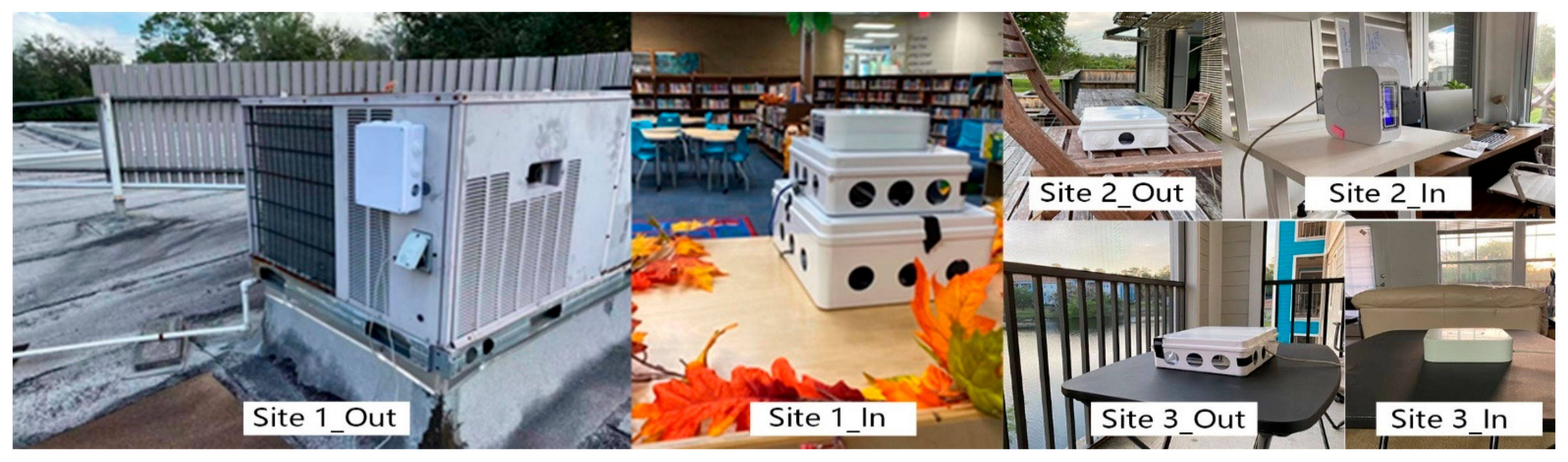
The three occupied sites (Table 1) chosen for this experiment were the media center of an elementary school building (Site 1), a lab house (Site 2), and a residential apartment unit (Site 3), which are all located in the city of Gainesville, Florida, United States. Gainesville is a mid-density city seat of central Florida, which stays in a humid subtropical climate throughout the year. The selected buildings for this study are mechanically conditioned all the year, and the windows are rarely opened to meet ANSI/ASHRAE Standard 52.2-2017 [8,36]. The buildings are located in the central region of the city to minimize the microclimate variation. Site-specific parameters are listed in Table 1. In total, the five air quality parameters monitored were PM2.5, PM10, NO2, relative humidity, and temperature. Three major monitoring protocols were followed to reduce measurement uncertainty, including the standardized EPA protocol for characterizing IAQ in large office buildings [37], the [38] for monitoring indoor air quality in schools (regional office for Europe), and requirements of the Schools Indoor Pollution and Health Observatory Network in Europe project (SINPHONIE) [39]. A two-week indoor and outdoor air quality measurement was carried out with ten-minute sampling intervals for 24 h continuously for all cases. For site 1, data were collected between 8 November 2019 and 22 November 2019 (before COVID-19). For site 2, data were collected between 4 August 2020 and 18 August 2020, while for site 3, air quality was monitored from 8 September 2020 to 22 September 2020. Each indoor monitor system was set up about 3.6 feet above the floor, 4.9 feet from any corners [37,40]. For comparison, outdoor air quality and RHT measurements were conducted simultaneously with indoor air measurement (Figure 1). For site 1, a weatherproofed sensor was placed 4.9 feet above the surface of the roof. For site 2, the outdoor sensor was placed 4.9 feet above the deck of the laboratory. Finally, for site 3, the sensor was placed 4 feet above balcony of an apartment [38,40,41].
2.2. Sensors
Two weatherproof Air Quality Egg (AQE, 2018) monitors manufactured by WickedDevice, LCC [42,43] were used to measure the concentration of indoor and outdoor pollutants as well as relative humidity (RH) and temperature (RHT) simultaneously for each site. This particular AQE was used because of its commercial availability, factory calibrated, and easy data accessibility and transmissions with lower purchase and operation cost [8,42]. In addition, according to the test reports from the US EPA and from the Air Quality Sensor Performance Evaluation Center (AQ-SPEC, SCAQMD), the field tests results of both laboratory showed that AQE sensors can provide reliable indoor air quality (IAQ) data with low intra-model variability and 100% data recovery [44,45,46,47]. Each AQE unit is assembled with a particulate matter module (Dual Plantower PMS5003), a CO module (3SP_CO_1000 Package 110-102), a NO2 module (3SP_NO2_5F P Package 110-507), and a RHT sensor (DHT22). The specifications of each sensor module are shown in Table 2.
2.3. Descriptive Statistics and Correlation Analysis
The indoor and outdoor environment parameters measured by the air quality monitors are subjected to descriptive statistics and correlation analysis using Python (version 3.6.12) language and Jupyter Notebooks. A quantile–quantile (Q-Q) plot graph was applied in Python to standardize reference data and test the data distribution [48,49]. The Spearman correlation coefficients were calculated to analyze the monotonic relationship and the inter-dependency between each pollutant on another [50,51]. The Spearman rank-order correlation coefficient (ρ) can be expressed as an equation [50]:
where di represents the difference between the corresponding ranks, and n is the number of data points. The coefficient value (r) ranges between −1 (highest negative correlation) and 1 (highest positive correlation), while a p-value less than 0.05 was considered statistically significant.
2.4. Principal Component Analysis (PCA)
PCA is a dimensionality reduction technique that elucidates the multicollinearity phenomenon among variables with a smaller set of uncorrelated variables called principal components (PCs) [35,52,53]. PCA can be used to validate the correlation between the original variables by determining the most significant parameters [54,55]. Each principal component is an orthogonal projection of the original variables, with a minimum loss of traits. The eigenvectors and eigenvalues of a covariance matrix are the main elements required for PCA to capture the visual orientations of new data points and their magnitude [56]. The eigenvalues λ, of the covariance matrix, is computed by the following expression [57,58]:
where det is the determinant of the matrix, I is the identity matrix, and C is the covariance matrix. Solving the above equation will result in k possible eigenvalues λ. The scores of PCs (eigenvectors) can be expressed as an equation [53,59,60]:
where Zir is the score for the ith data point on the rth principal component, α is the component loading, x is the variable, and k is the total number of variables. In this study, we focused specifically on identifying factors that affect the indoor PM2.5, PM10, and NO2 concentrations during the measurement periods. PCA and linear regression were used to validate the correlation analysis results and determine the significant independent variables contributing to the degradation of target pollutants. A PCA and biplot-based data visualization were carried out using the Scikit-learn machine learning library and the yellow-brick visualizer in Python [61].
3. Results and Discussion
3.1. PM2.5, PM10, and NO2 Concentrations
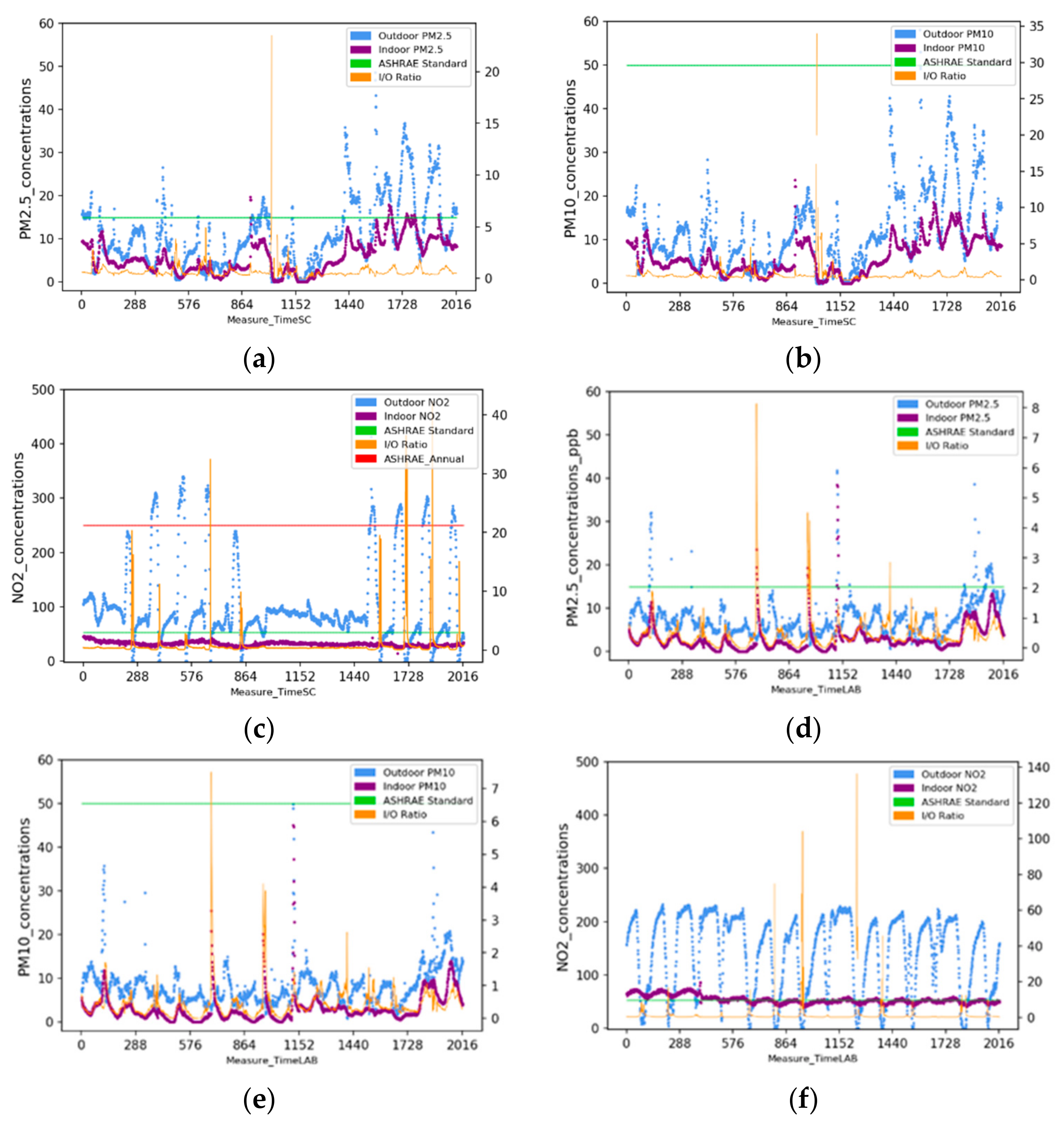
The measured average indoor and outdoor environmental parameters along with their standard deviation, minimum, maximum, and indoor to the outdoor ratio (I/O ratio), are presented in Table 3 and Table 4. The mean temperature indoors during the monitoring period was not significantly different among the locations. Site 1 observed the lowest average humidity of 44.7%, while site 2 and site 3 were 67.7% and 53.5%, respectively. The average indoor PM2.5 and PM10 concentrations for site 1 were 5.85 and 6.09 µg/m3, while site 2 has comparatively lower average values at 3.04 and 3.18 µg/m3. The highest means and standard deviations of indoor PM2.5 and PM10 (13.0 ± 30.2 µg/m3; 15.0 ± 35.3 µg/m3) were observed in site 3. For both sites 1 and 2, the recorded mean of indoor PM2.5 and PM10 concentrations were lower than outdoor PM2.5 and PM10 concentrations. Conversely, mean PM2.5, PM10, and NO2 concentrations were higher indoors than outdoors in the residential building (site 3). The indoor concentrations of NO2 at each site ranged from 14.8 to 46.5 ppb, 38.7 to 86.3 ppb, and 30.9 to 69.3 ppb. In all cases, the mean outdoor NO2 values were significantly higher than indoors.
Time series of indoor and outdoor PM2.5, PM10, and NO2 concentrations measured during the sampling periods are plotted in Figure 2. The majority of indoor PM2.5 and PM10 concentrations for all the sites met the minimum requirements of the ASHRAE 62.1-2019 standard, which is 35 µg/m3 (24 h mean) for PM2.5 and 50 µg/m3 (24 h mean) for PM10 [8,62]. The crests with unhealthy levels of indoor PM2.5 at site 3 may be attributed to regular household cooking and human behavior activities (lunch or dinner break) [63,64,65]. The overall trends between indoor and outdoor particulate matter (PM2.5 and PM10) concentrations were similar for site 1 and 2. It can be seen from Figure 2d,e that there is a time-delay affected peaks shift between indoor and outdoor particulate matter (PM2.5 and PM10) values in site 2 (office room). The potential reason for this trend might be due to the city traffic in rush hours, since site 2 has the shortest distance to the nearest busy road among all sites while having sedentary human behavior during working hours [66,67]. The time-series concentration for NO2 shows a significantly stable pattern than the outdoor concentration values for all sites due to a lack of indoor emitting sources [17]. Except for site 2, which is close to a busy road, most of the indoor concentration values for NO2 lie below the index of ASHRAE 62.1-2019 standard 53 ppb (1-year mean) and 100 ppb (1-h mean) [8,62].
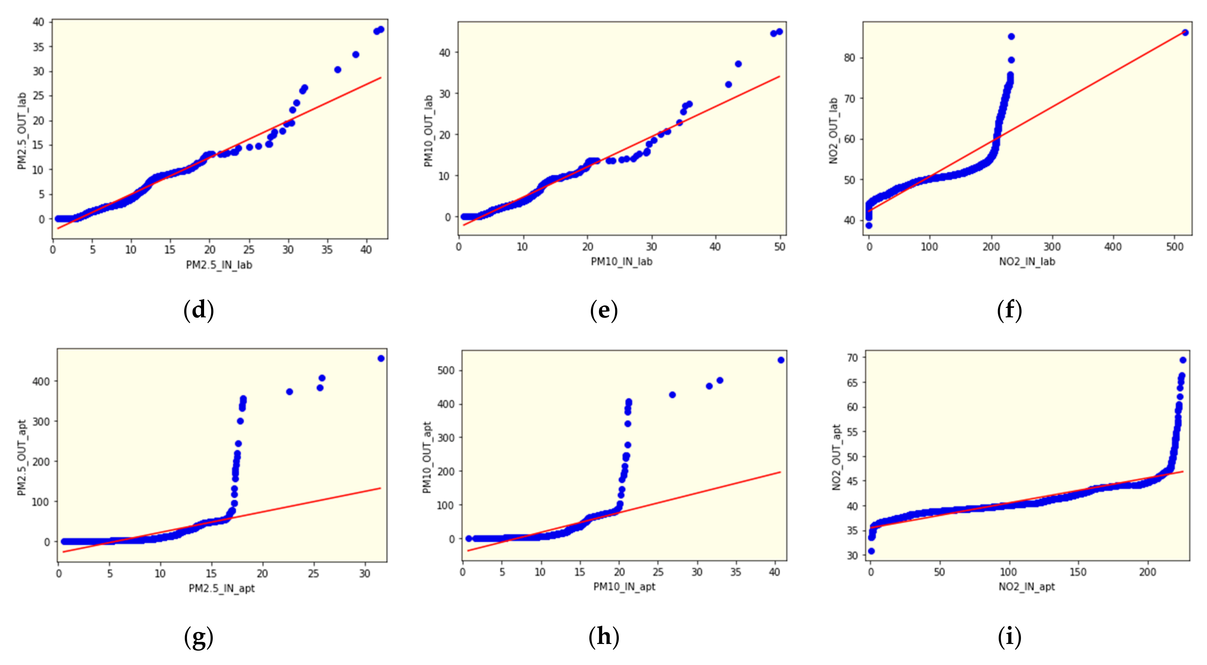
3.2. Quantile–Quantile (Q-Q) Plot
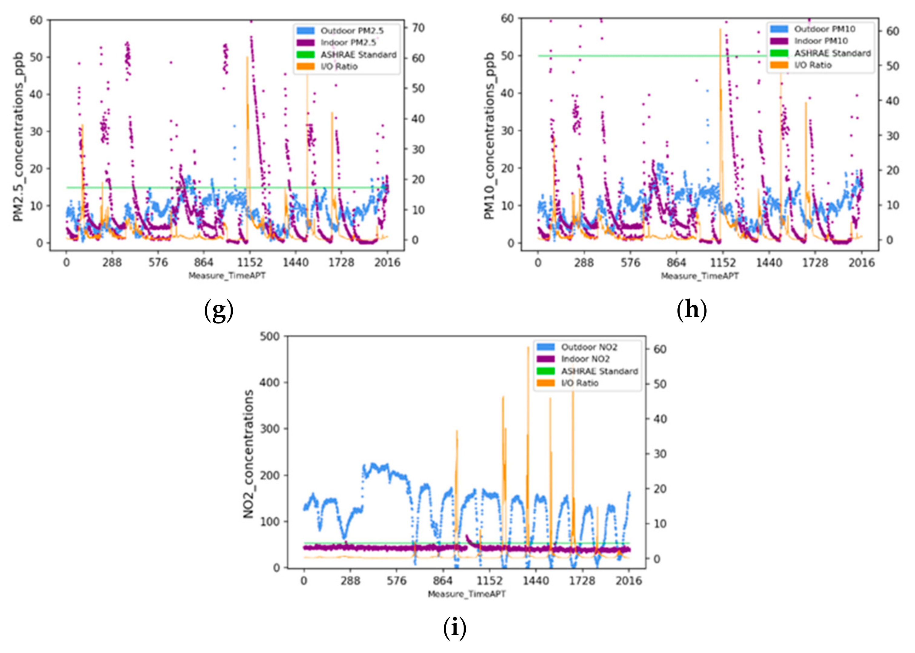
Figure 3 represents quantile–quantile (Q-Q) plots applied to verify and visualize the distributional difference between indoor air quality data and the corresponding outdoor data by plotting their quantiles against each other [48]. The type of data distribution can be determined by characterizing the spatial pattern of the normalized data points. If two set distributions are mostly similar (normally distributed), then plots of the quantiles of distributions will fall close to the identity line [48,49]. Different type of distributions leads to various deviation ratios. From Figure 3a–c, the site 1 (indoor and outdoor) data are normally distributed with a small deviation from the identity line. In Figure 3d–f, which represents site 2, the quantile plots of the distribution of indoor and outdoor pollutants show a skewed distribution with low and high degrees of variation from the identity line toward higher concentrations. For site 3, the PM2.5 and PM10 data are clustered along the low-to-medium spectrum of the data range, while positive deviations (site 3) were found between the higher concentration range. Figure 3i shows that the distribution of NO2 indoor and outdoor concentrations is highly concentrated along the identity line.
3.3. Correlation Analysis
The Spearman rank-based correlation was used to extract the nonparametric relationship to outcome the probabilistic association between target parameters by assigning a coefficient value bounded between −1 and 1 [50,51]. According to Figure 4, site 1 and site 2 reveal a stronger correlation between indoor and outdoor measurements compared to site 3. Significant positive correlations were found between indoor NO2 and indoor relative humidity (Rsite1 = 0.85, Rsite2 = 0.99, Rsite3 = 0.77) at all sites. NO2 has the propensity to react with water vapor appear in building structures, which may lead to an increase in NO2 concentrations [68,69]. This positive trend can also be found at site 2 and site 3 among indoor NO2 and outdoor NO2 (Rsite2 = 0.87, Rsite3 = 0.7), while site 1 shows a negligible correlation between them. Both sites 1 and 2 have a high degree of positive correlation between indoor particulate matters (PM2.5 and PM10) and corresponding outdoor values (Rsite1_pm2.5 = 0.65, Rsite2 pm2.5 = 0.64, Rsite1_pm10 = 0.64, Rsite2_pm10 = 0.56). Many relevant studies reported similar positive correlation value between indoor and outdoor PM concentrations in public buildings. Site 3 shows a high negative correlation between indoor and outdoor particulate matters (PM2.5 and PM10). The similar negative correlation between indoor and outdoor PM within a mechanical ventilated living space was observed in serial studies [16,70,71]. This indicates that the indoor PM values are affected significantly by day-to-day household activities compared to educational and office spaces [72,73,74].
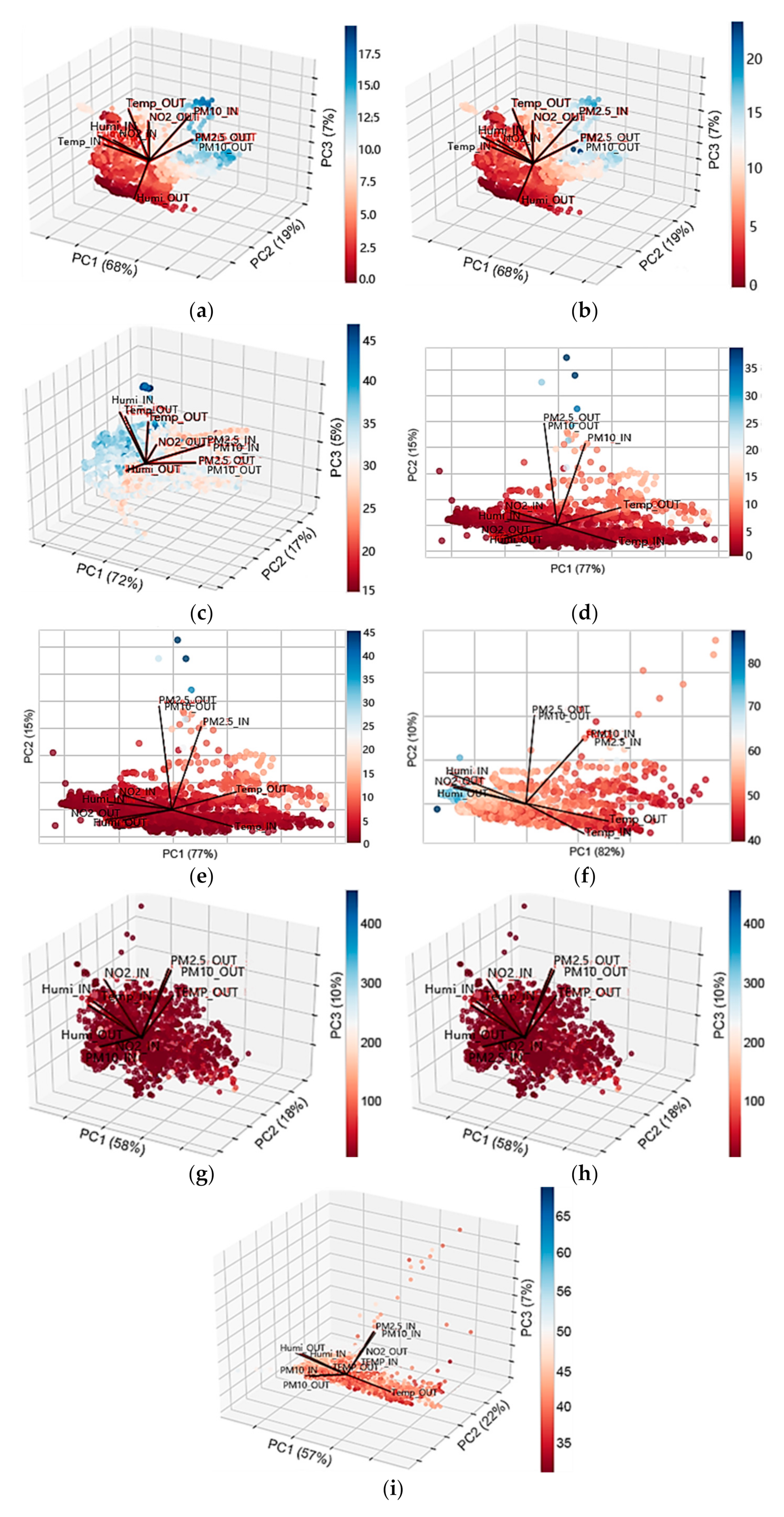
3.4. Biplot–PCA for Site 1, 2, 3
A PCA-based multivariate linear regression model was employed for parameters such as PM2.5, PM10, NO2, and temperature and humidity for both indoor and outdoor test conditions [32,33]. This was used to evaluate results obtained from the correlation analysis [52,56]. The measured values are utilized to formulate a multidimensional dataset, which is projected onto a biplot. A biplot is a scatter plot that depicts the relationship between observed data and dependent variables in terms of principal components [34,35]. In a PCA-based biplot, points are the projected observations, vectors are the projected variables. However, biplot cannot be used to estimate the exact coordinates because the vectors have been centered and scaled. The multivariate dataset was dimensionally redacted down into 3D and 2D plots where the above-mentioned parameters were plotted with respect to indoor PM2.5, PM10, and NO2. In order to plot the biplot, PCA results are to be interpreted, which is followed by identifying the number of principal components [35]. Sites 1 and 3 are represented in 3D plots as the sum of the first, second, and third principal components, which result in an aggregate of less than 90%. Whereas for site 2, PC1 and PC2 sum to more than 90% and hence are represented as a 2D plot. Figure 5a,b display similar variance across the first, second, and third principal components. This can be attributed to the close dependency of PM2.5 to PM10 in site 1. This trend is also observed in site 2 (Figure 5d,e) and site 3 (Figure 5g,h). Site 2 shows the highest NO2 principal component values at PC1 = 82%.
Table 5 depicts PCA-based linear regression analysis coefficient values for all three sites with respect to indoor PM2.5, PM10, and NO2 with 95% confidence interval. The linear regression results are in an agreement with the Spearman inter-parameter correlation. Three levels of statistical significance, 0.001, 0.05, and 0.1 in decreasing order of significance were observed. Indoor PM2.5 and PM10 show a strong dependence with site 1; this trend can be witnessed similarly in the Spearman correlation matrix. NO2 for site 1 shows negative principal component values, which is similar to the correlation values (r) obtained through Spearman correlation. The first and second principal component numbers for site 2 for PM2.5 and PM10 are almost identical. Likewise, from Figure 4, PM2.5 and PM10 are strongly correlated. This may be attributed to the minimal occupant behavior owing to quarantine protocol restricting the active maximum number of occupants to 1 at a given time. For site 2, NO2 possesses contradictory first and second principal component numbers (PC1 = −0.255, p < 0.001, and PC2 = 0.135, p < 0.001). This pattern can be consistently observed from the Spearman correlation as well. Site 3 has weak dependence across all three principal component numbers, while PC3 displays the least significance amongst all sites. This is contrasting from the indoor NO2, outdoor NO2, and relative humidity observed from the correlation heatmap. Site 1 and Site 2 show an overall stronger inter-parameter dependence, which is also witnessed from the PCA-based linear regression analysis. A relatively weaker correlation among parameters is displayed by the residential building (site 3). There is a mismatch between results derived from the PCA (site 3) and the values of the corresponding correlation coefficient. The proposed study could contribute to developing efficient solutions to identify and verify the significant variables that affect indoor air pollutant concentrations in buildings, such as windows operation, ventilation control, and building material selections.
4. Conclusions
The purpose of this study was to introduce a biplot-based PCA approach that could serve as a novel method to visualize and validate the relations between indoor and outdoor air quality data. PM2.5, PM10, NO2, and RHT data were collected continuously in three different building types (Supplementary Materials: elementary school—site 1, laboratory—site 2, and residential—site 3) with a span of two weeks. The highest means and standard deviations of indoor PM2.5 and PM10 (13.0 ± 30.2 µg/m3; 15.0 ± 35.3 µg/m3) were observed in site 3. For both sites 1 and 2, the recorded mean of indoor PM2.5 and PM10 concentrations were lower than outdoors. The average indoor NO2 levels were significantly lower and steadier than outdoors. The Spearman coefficients showed a stronger correlation among these target environmental measurements on sites 1 and 2, while it showed a weaker correlation on site 3. Three and two principal components were found for sites 1 and 3, and site 2, respectively, from the biplot-based PCA. The PCA-based linear regression results showed higher dependency for site 1 and site 2 (p < 0.001) when compared to the Spearman correlation values (r) and showed a lower dependency for site 3. The results displayed a mismatch between the PCA-based regression and Spearman correlation for site 3. The method utilized in this research can be implemented in studies and analyzes high volumes of multiple building environmental measurements along with optimized visualization. For further studies, building characteristics, occupant behaviors, and seasonal variations with a larger sample size are recommended to be included in order for better understanding and analyzing the relationships between indoor and outdoor air quality.
Supplementary Materials
The following are available online at https://0-www-mdpi-com.brum.beds.ac.uk/article/10.3390/buildings11050218/s1.
Author Contributions
Conceptualization: H.Z.; Data collection and analysis: H.Z.; Writing—Original draft: H.Z.; writing—Review and editing: R.S.; supervision: R.S. All authors have read and agreed to the published version of the manuscript.
Funding
This research received no external funding.
Institutional Review Board Statement
Not applicable.
Informed Consent Statement
Not applicable.
Data Availability Statement
The data presented in this study are available in Supplementary Materials.
Conflicts of Interest
The authors declare no conflict of interest.
References
- WHO. Ambient Air Pollution Attributable Death Rate (Per 100,000 Population), World Health Organization. Available online: https://www.who.int/data/gho/data/indicators/indicator-details/GHO/ambient-air-pollution-attributable-death-rate-(per-100-000-population) (accessed on 26 February 2021).
- Ritchie, H.; Roser, M. Indoor Air Pollution. Available online: https://ourworldindata.org/indoor-air-pollution (accessed on 3 February 2021).
- US-EPA. Report on the Environment: What Are the Trends in Indoor Air Quality and Their Effects on Human Health? Available online: https://www.epa.gov/report-environment/indoor-air-quality (accessed on 3 November 2020).
- US-EPA. The Inside Story: A Guide to Indoor Air Quality. Available online: https://www.cpsc.gov/Safety-Education/Safety-Guides/Home/The-Inside-Story-A-Guide-to-Indoor-Air-Quality (accessed on 20 June 2020).
- Deng, S.; Lau, J. Seasonal variations of indoor air quality and thermal conditions and their correlations in 220 classrooms in the Midwestern United States. Build. Environ. 2019, 157, 79–88. [Google Scholar] [CrossRef]
- Seppanen, O.; Fisk, W.J. Relationship of SBS-Symptoms and Ventilation System Type in Office Buildings; Lawrence Berkeley National Laboratory: Berkeley, CA, USA, 2002; pp. 1–8. [Google Scholar]
- Saeki, Y.; Kadonosono, K.; Uchio, E. Clinical and allergological analysis of ocular manifestations of sick building syndrome. Clin. Ophthalmol. 2017, 11, 517–522. [Google Scholar] [CrossRef] [Green Version]
- Zhang, H.; Srinivasan, R. A systematic review of air quality sensors, guidelines, and measurement studies for indoor air quality management. Sustainability 2020, 12, 9045. [Google Scholar] [CrossRef]
- NAAQS. Primary National Ambient Air Quality Standard (NAAQS) for Sulfur Dioxide. Available online: https://www.epa.gov/so2-pollution/primary-national-ambient-air-quality-standard-naaqs-sulfur-dioxide (accessed on 26 July 2019).
- Correia, G.; Rodrigues, L.; Gameiro da Silva, M.; Gonçalves, T. Airborne route and bad use of ventilation systems as non-negligible factors in SARS-CoV-2 transmission. Med. Hypotheses 2020, 141, 109781. [Google Scholar] [CrossRef] [PubMed]
- Venter, Z.S.; Aunan, K.; Chowdhury, S.; Lelieveld, J. COVID-19 lockdowns cause global air pollution declines with implications for public health risk. medRxiv 2020, 18984–18990. [Google Scholar] [CrossRef] [Green Version]
- Wu, X.; Nethery, R.C.; Sabath, M.B.; Braun, D.; Dominici, F. Exposure to air pollution and COVID-19 mortality in the United States: A nationwide cross-sectional study. medRxiv 2020, 1–36. [Google Scholar] [CrossRef] [Green Version]
- Ge, Z.-Y.; Yang, L.-M.; Xia, J.-J.; Fu, X.-H.; Zhang, Y.-Z. Possible aerosol transmission of COVID-19 and special precautions in dentistry. J. Zhejiang Univ. Sci. B 2020, 21, 361–368. [Google Scholar] [CrossRef] [Green Version]
- Travaglio, M.; Yu, Y.; Popovic, R.; Leal, N.S.; Martins, L.M. Links between air pollution and COVID-19 in England. medRxiv 2020, 115859. [Google Scholar] [CrossRef]
- EPA. Building Air Quality—A Guide for Building Owners and Facility Managers; EPA: Washington, DC, USA, 1991; pp. 1–228.
- Deng, G.; Li, Z.; Wang, Z.; Gao, J.; Xu, Z.; Li, J.; Wang, Z. Indoor/outdoor relationship of PM2.5 concentration in typical buildings with and without air cleaning in Beijing. Indoor Built Environ. 2017, 26, 60–68. [Google Scholar] [CrossRef]
- Shields, K.N.; Cavallari, J.M.; Hunt, M.J.O.; Lazo, M.; Molina, M.; Molina, L.; Holguin, F. Traffic-related air pollution exposures and changes in heart rate variability in Mexico City: A panel study. Environ. Health 2013, 12, 1–14. [Google Scholar] [CrossRef] [Green Version]
- Bluyssen, P.M.; Cox, C.; Seppänen, O.; Fernandes, E.D.O.; Clausen, G.; Müller, B.; Roulet, C.-A. Why, when and how do HVAC-systems pollute the indoor environment and what to do about it? The European AIRLESS project. Build. Environ. 2003, 38, 209–225. [Google Scholar] [CrossRef]
- De Robles, D.; Kramer, S.W. Improving Indoor Air Quality through the Use of Ultraviolet Technology in Commercial Buildings. Procedia Eng. 2017, 196, 888–894. [Google Scholar] [CrossRef]
- Zhang, X.; Zhang, W.; Yi, M.; Wang, Y.; Wang, P.; Xu, J.; Lin, F. High-performance inertial impaction filters for particulate matter removal. Sci. Rep. 2018, 8, 4757. [Google Scholar] [CrossRef] [PubMed]
- Morawska, L.; Thai, P.K.; Liu, X.; Asumadu-Sakyi, A.; Ayoko, G.; Bartonova, A.; Bedini, A.; Chai, F.; Christensen, B.; Dunbabin, M.; et al. Applications of low-cost sensing technologies for air quality monitoring and exposure assessment: How far have they gone? Environ. Int. 2018, 116, 286–299. [Google Scholar] [CrossRef]
- Wang, Z.; Delp, W.W.; Singer, B.C. Performance of low-cost indoor air quality monitors for PM2.5 and PM10 from residential sources. Build. Environ. 2020, 171, 106654. [Google Scholar] [CrossRef]
- Williams, R. EPA Tools and Resources Webinar, Low Cost Air Quality Sensors; EPA: Washington, DC, USA, 2019.
- Chatzidiakou, L.; Krause, A.; Popoola, O.; Di Antonio, A.; Kellaway, M.; Han, Y.; Squires, F.; Wang, T.; Zhang, H.; Wang, Q.; et al. Characterising low-cost sensors in highly portable platforms to quantify personal exposure in diverse environments. Atmos. Meas. Tech. 2019, 12, 4643–4657. [Google Scholar] [CrossRef] [Green Version]
- Nezis, I.; Biskos, G.; Eleftheriadis, K.; Kalantzi, O.I. Particulate matter and health effects in offices—A review. Build. Environ. 2019, 156, 62–73. [Google Scholar] [CrossRef]
- Chamseddine, A.; Alameddine, I.; Hatzopoulou, M.; El-Fadel, M. Seasonal variation of air quality in hospitals with indoor–outdoor correlations. Build. Environ. 2019, 148, 689–700. [Google Scholar] [CrossRef] [Green Version]
- Gabriel, M.F.; Felgueiras, F.; Mourão, Z.; Fernandes, E.O. Assessment of the air quality in 20 public indoor swimming pools located in the Northern Region of Portugal. Environ. Int. 2019, 133, 105274. [Google Scholar] [CrossRef]
- Zhao, Y.; Song, X.; Wang, Y.; Zhao, J.; Zhu, K. Seasonal patterns of PM10, PM2.5, and PM1.0 concentrations in a naturally ventilated residential underground garage. Build. Environ. 2017, 124, 294–314. [Google Scholar] [CrossRef]
- Kim, J.; Kong, M.; Hong, T.; Jeong, K.; Lee, M. The effects of filters for an intelligent air pollutant control system considering natural ventilation and the occupants. Sci. Total Environ. 2019, 657, 410–419. [Google Scholar] [CrossRef] [PubMed]
- Madureira, J.; Paciência, I.; Pereira, C.; Teixeira, J.P.; Fernandes, E.D.O. Indoor air quality in Portuguese schools: Levels and sources of pollutants. Indoor Air 2016, 26, 526–537. [Google Scholar] [CrossRef] [Green Version]
- Kwon, S.-B.; Jeong, W.; Park, D.; Kim, K.-T.; Cho, K.H. A multivariate study for characterizing particulate matter (PM10, PM2.5, and PM1) in Seoul metropolitan subway stations, Korea. J. Hazard. Mater. 2015, 297, 295–303. [Google Scholar] [CrossRef] [PubMed]
- Chen, Y.T.; Shrestha, S. Source Classification of Indoor Air Pollutants Using Principal Component Analysis for Smart Home Monitoring Applications. In Proceedings of the 2018 IEEE International Conference on Electro/Information Technology (EIT), Rochester, MI, USA, 3–5 May 2018; pp. 129–133. [Google Scholar] [CrossRef]
- Ul-Saufie, A.Z.; Yahaya, A.S.; Ramli, N.A.; Rosaida, N.; Hamid, H.A. Future daily PM10 concentrations prediction by combining regression models and feedforward backpropagation models with principle component analysis (PCA). Atmos. Environ. 2013, 77, 621–630. [Google Scholar] [CrossRef]
- Braak, C.; Ter, J.F. Principal Components Biplots and Alpha and Beta Diversity, Wiley on behalf of the Ecological Society of America. Bioinformatics 2005, 21, 454–462. [Google Scholar]
- Hron, K.; Jelínková, M.; Filzmoser, P.; Kreuziger, R.; Bednář, P.; Barták, P. Statistical analysis of wines using a robust compositional biplot. Talanta 2012, 90, 46–50. [Google Scholar] [CrossRef]
- ASHRAE. ASHRAE 62.1 The Standards for Ventilation and Indoor Air Quality. Available online: https://www.ashrae.org/technical-resources/bookstore/standards-62-1-62-2 (accessed on 4 April 2020).
- EPA. A Standardized EPA Protocol for Characterizing Indoor Air Quality in Large Office Buildings; EPA: Washinton, DC, USA, 2016.
- WHO. Methods for Monitoring Indoor Air Quality in Schools; WHO: Bonn, Germany, 2011. [Google Scholar]
- SINPHONIE. The Schools Indoor Pollution and Health Observatory Network in Europe (SINPHONIE) Project; Publications Office of the European Union: Luxembourg, 2014. [Google Scholar]
- Zhang, H.; Srinivasan, R.; Ganesan, V. Low cost, multi-pollutant sensing system using raspberry pi for indoor air quality monitoring. Sustainability 2021, 13, 370. [Google Scholar] [CrossRef]
- Roshan, S.K.; Godini, H.; Nikmanesh, B.; Bakhshi, H.; Charsizadeh, A. Study on the relationship between the concentration and type of fungal bio-aerosols at indoor and outdoor air in the Children’s Medical Center, Tehran, Iran. Environ. Monit. Assess. 2019, 191, 48. [Google Scholar] [CrossRef]
- AQ-SPEC. Air Quality Egg Evaluation Summary; AQ-SPEC: Diamond Bar, CA, USA, 2019. [Google Scholar]
- AQ-SPEC. Laboratory Evaluation Air Quality Egg 2018 Model; AQ-SPEC: Diamond Bar, CA, USA, 2018. [Google Scholar]
- Stewart, D.R.; Saunders, E.; Perea, R.; Fitzgerald, R.; Campbell, D.E.; Stockwell, W.R. Projected changes in particulate matter concentrations in the South Coast Air Basin due to basin-wide reductions in nitrogen oxides, volatile organic compounds, and ammonia emissions. J. Air Waste Manag. Assoc. 2019, 69, 192–208. [Google Scholar] [CrossRef] [PubMed]
- SCAQMD. South Coast Air Quality Mnanagement District Draft Staff Report for 2015 8-Hour Ozone Standard Reasonably Available Control Technology (RACT) Demonstration APRIL 2020; SCAQMD: Diamond Bar, CA, USA, 2020. [Google Scholar]
- AQ-SPEC. Field Evaluation uHoo PM2.5, Ozone, and CO Sensor; AQ-SPEC: Diamond Bar, CA, USA, 2019. [Google Scholar]
- AQSPEC. Field Evaluation Air Quality Egg v.2 Particulate Matter; AQSPEC: Diamond Bar, CA, USA, 2018. [Google Scholar]
- Oldford, R.W. Self-Calibrating Quantile–Quantile Plots. Am. Stat. 2016, 70, 74–90. [Google Scholar] [CrossRef]
- Augustin, N.H.; Sauleau, E.A.; Wood, S.N. On quantile quantile plots for generalized linear models. Comput. Stat. Data Anal. 2012, 56, 2404–2409. [Google Scholar] [CrossRef] [Green Version]
- Akoglu, H. User’s guide to correlation coefficients. Turk. J. Emerg. Med. 2018, 18, 91–93. [Google Scholar] [CrossRef]
- Gauthier, T.D. Detecting trends using spearman’s rank correlation coefficient. Environ. Forensics 2001, 2, 359–362. [Google Scholar] [CrossRef]
- Kriegel, H.P.; Kröger, P.; Schubert, E.; Zimek, A. A general framework for increasing the robustness of PCA-based correlation clustering algorithms. In Proceedings of the International Conference on Scientific and Statistical Database Management 2008, Hong Kong, China, 9–11 July 2008; pp. 418–435. [Google Scholar] [CrossRef] [Green Version]
- Holand, S.M. PRINCIPAL COMPONENTS ANALYSIS (PCA); University of Georgia: Athens, GA, USA, 2019. [Google Scholar]
- Wold, S.; Esbensen, K.; Geladi, P. Principal component analysis. Chemom. Intell. Lab. Syst. 1987, 2, 37–52. [Google Scholar] [CrossRef]
- Pires, J.C.M.; Martins, F.G.; Sousa, S.I.V.; Alvim-Ferraz, M.C.M.; Pereira, M.C. Selection and validation of parameters in multiple linear and principal component regressions. Environ. Model. Softw. 2008, 23, 50–55. [Google Scholar] [CrossRef]
- Paul, L.C.; Suman, A.A.; Sultan, N. Methodological Analysis of Principal Component Analysis (PCA) Method. IJCEM Int. J. Comput. Eng. Manag. 2013, 16, 2230–7893. [Google Scholar]
- Ringnér, M. What is principal component analysis? Nat. Biotechnol. 2008, 26, 303–304. [Google Scholar] [CrossRef] [PubMed]
- Abdi, H.; Williams, L.J. Computational Statistics: Principal component analysis. Wiley Interdiscip. Rev. 2010, 2, 433–459. [Google Scholar] [CrossRef]
- Smith, L. A Tutorial on PCSA; Department of Computer Science, University of Otago: Dunedin, New Zealand, 2006; pp. 12–28. [Google Scholar]
- Kim, M.; Sankararao, B.; Kang, O.; Kim, J.; Yoo, C. Monitoring and prediction of indoor air quality (IAQ) in subway or metro systems using season dependent models. Energy Build. 2012, 46, 48–55. [Google Scholar] [CrossRef]
- Bengfort, B.; Bilbro, R. Yellowbrick: Visualizing the Scikit-Learn Model Selection Process. J. Open Source Softw. 2019, 4, 1075. [Google Scholar] [CrossRef]
- ANSI-ASHRAE. ANSI/ASHRAE Standard 62.1-2019, Ventilation for Acceptable Indoor Air Quality; American Society of Heating, Refrigerating and Air-Conditioning Engineers: Atlanta, GA, USA, 2019. [Google Scholar]
- Zhou, Z.; Liu, Y.; Yuan, J.; Zuo, J.; Chen, G.; Xu, L.; Rameezdeen, R. Indoor PM2.5 concentrations in residential buildings during a severely polluted winter: A case study in Tianjin, China. Renew. Sustain. Energy Rev. 2016, 64, 372–381. [Google Scholar] [CrossRef]
- Jedrychowski, W.A.; Perera, F.P.; Pac, A.; Jacek, R.; Whyatt, R.M.; Spengle, J.D.; Dumyahn, T.S.; Sochacka-Tatara, E. Variability of total exposure to PM2.5 related to indoor and outdoor pollution sources: Krakow study in pregnant women. Sci. Total Environ. 2006, 366, 47–54. [Google Scholar] [CrossRef]
- Song, P.; Wanga, L.; Hui, Y.; Li, R. PM2.5 Concentrations Indoors and Outdoors in Heavy Air Pollution Days in Winter. Procedia Eng. 2015, 121, 1902–1906. [Google Scholar] [CrossRef] [Green Version]
- Martuzevicius, D.; Grinshpun, S.A.; Lee, T.; Hu, S.; Biswas, P.; Reponen, T.; LeMasters, G. Traffic-related PM2.5 aerosol in residential houses located near major highways: Indoor versus outdoor concentrations. Atmos. Environ. 2008, 42, 6575–6585. [Google Scholar] [CrossRef]
- Chao, C.Y.; Wong, K.K. Residential indoor PM10 and PM2.5 in Hong Kong and the elemental composition. Atmos. Environ. 2002, 36, 265–277. [Google Scholar] [CrossRef]
- NAAQS. Primary National Ambient Air Quality Standards (NAAQS) for Nitrogen Dioxide. Available online: https://www.epa.gov/no2-pollution/primary-national-ambient-air-quality-standards-naaqs-nitrogen-dioxide (accessed on 4 May 2020).
- Spengler, J.D.; Ferris, B.G.; Dockery, D.W.; Speizer, F.E. Sulfur Dioxide and Nitrogen Dioxide Levels Inside and Outside Homes and the Implications on Health Effects Research. Environ. Sci. Technol. 1979, 13, 1276–1280. [Google Scholar] [CrossRef]
- Goyal, R.; Khare, M. Indoor-outdoor concentrations of RSPM in classroom of a naturally ventilated school building near an urban traffic roadway. Atmos. Environ. 2009, 43, 6026–6038. [Google Scholar] [CrossRef]
- Nadali, A.; Arfaeinia, H.; Asadgol, Z.; Fahiminia, M. Indoor and outdoor concentration of PM10, PM2.5 and PM1 in residential building and evaluation of negative air ions (NAIs) in indoor PM removal. Environ. Pollut. Bioavailab. 2020, 32, 47–55. [Google Scholar] [CrossRef] [Green Version]
- McCormack, M.C.; Breysse, P.N.; Hansel, N.N.; Matsui, E.C.; Tonorezos, E.S.; Curtin-Brosnan, J.; Williams, D.L.; Buckley, T.J.; Eggleston, P.A.; Diette, G.B. Common household activities are associated with elevated particulate matter concentrations in bedrooms of inner-city Baltimore pre-school children. Environ. Res. 2008, 106, 148–155. [Google Scholar] [CrossRef] [Green Version]
- Pennise, D.; Brant, S.; Agbeve, S.M.; Quaye, W.; Mengesha, F.; Tadele, W.; Wofchuck, T. Indoor air quality impacts of an improved wood stove in Ghana and an ethanol stove in Ethiopia. Energy Sustain. Dev. 2009, 13, 71–76. [Google Scholar] [CrossRef]
- Chen, Q.; Hildemann, L.M. The effects of human activities on exposure to particulate matter and bioaerosols in residential homes. Environ. Sci. Technol. 2009, 43, 4641–4646. [Google Scholar] [CrossRef] [PubMed]
Figure 1.
Photos of field monitoring.

Figure 2.
Two weeks evaluation of indoor and outdoor pollutants monitored at 10-min intervals (144 observational points a day equating to 2016): (a) Site 1-PM2.5, (b) Site 1-PM10, (c) Site 1-NO2, (d) Site 2-PM2.5, (e) Site 2-PM10, (f) Site 2-NO2, (g) Site 3-PM2.5, (h) Site 3-PM10, (i) Site 3-NO2.
Figure 2.
Two weeks evaluation of indoor and outdoor pollutants monitored at 10-min intervals (144 observational points a day equating to 2016): (a) Site 1-PM2.5, (b) Site 1-PM10, (c) Site 1-NO2, (d) Site 2-PM2.5, (e) Site 2-PM10, (f) Site 2-NO2, (g) Site 3-PM2.5, (h) Site 3-PM10, (i) Site 3-NO2.


Figure 3.
Quantile-Quantile (Q-Q) plot of indoor-outdoor data: (a) Site 1-PM2.5, (b) Site 1-PM10, (c) Site 1-NO2, (d) Site 2-PM2.5, (e) Site 2-PM10, (f) Site 2-NO2, (g) Site 3-PM2.5, (h) Site 3-PM10, (i) Site 3-NO2. With an identity line (y = x, which acts as reference to standardize the axis).
Figure 3.
Quantile-Quantile (Q-Q) plot of indoor-outdoor data: (a) Site 1-PM2.5, (b) Site 1-PM10, (c) Site 1-NO2, (d) Site 2-PM2.5, (e) Site 2-PM10, (f) Site 2-NO2, (g) Site 3-PM2.5, (h) Site 3-PM10, (i) Site 3-NO2. With an identity line (y = x, which acts as reference to standardize the axis).


Figure 4.
Spearman correlation heat map for indoor and outdoor environmental parameters at three sites.
Figure 4.
Spearman correlation heat map for indoor and outdoor environmental parameters at three sites.

Figure 5.
PCA-based biplot of indoor–outdoor data: (a) Site 1-PM2.5, (b) Site 1-PM10, (c) Site 1-NO2, (d) Site 2-PM2.5, (e) Site 2-PM10, (f) Site 2-NO2, (g) Site 3-PM2.5, (h) Site 3-PM10, (i) Site 3-NO2. With calibrated axes and observations as scatters. The color bar represents the values of the dependent variable (target pollutant). The direction of eigenvectors is represented as solid red lines.


Table 1.
Building-related specifications at each site.
| Building Type | Elementary School (Site 1) | Lab (Site 2) | Residential (Site 3) |
|---|---|---|---|
| Space Type | Media Center | Office Room | Living Room |
| Room Size | 1180 sq.ft 18′8″ | Space floor area: 321 sq.ft Height: 11′4″ | Space floor area: 421 sq.ft Height: 9′6″ |
| Floor material | Carpet | Plywood | Carpet |
| HVAC Model | Carrier 50HJ-(008-14) 3 Ton Single-Package RTU; | Mitsubishi PEA-A18AA –1.5-ton concealed CLG. Ducted UNIT W/DUCT BOX& Registers; MITSUBISHI MXZ-3A30N | GOODMAN GSX130481 4-tons 2 Ton Central Air Conditioner Air Handler Unit GOODMAN Model AWUF24051BA |
| Number of AHU/room | 2 | 1 | 1 |
| Air flow rate plan: | 1500 CFM | 635 CFM | 835 CFM |
| Air Filter | Dual-Ply Filter Media (Dustlok) | PP Honeycomb fabric (washable) | AAF Flanders: PREpleat® LPD SC |
| Air Filter Level | MERV-9 | MERV-8 | MERV-8 |
| PM2.5 absorption capability | 35%–50% | 20%–35% | 20%–35% |
| Distance to nearest major road | 1383.25 ft. | 244.62 ft. | 1827.51 ft. |
| No. of windows | n/a | 3 | 2 |
| Indoor smoking | Not allowed | Not allowed | Not allowed |
Table 2.
Specifications of multi-sensor modules of Air Quality Egg version 2.
| Measured Parameter | Example Product | Manufacturer | Measurement Tolerance/Repeatability | Measuring Range | Circuit Voltage | Response Time |
|---|---|---|---|---|---|---|
| PM2.5; PM10 | PMS5003 | Plantower | ± 10%@ 100–500 μg/m3; ± 10 μg/m3 @0–100 μg/m3 | 0~500 µg/m3; ≥ 1000 µg/m3 | 5.0–5.5v | 10 s |
| NO2 | 3SP_NO2_5F P Package | SPEC sensors | <± 5% of reading or 10 ppb | 0–5 ppm | 10 to 50 uW | < 15 s |
| CO | 3SP_CO_1000 Package | SPEC sensors | <± 2% of reading | 0 to 1000 ppm | 10 to 50 uW | < 30 s (15 s typical) |
| RHT | DHT22 | Aosong Electronics | ± 0.5 °C and ± 1% | 40 °C to 80 °C; 0% to 100% | 3.5–5.5 v | 2 s |
Table 3.
Descriptive statistics of indoor environmental parameters measured at sites 1, 2, and 3.
| Site 1 | Site 2 | Site 3 | |||||||||||||
|---|---|---|---|---|---|---|---|---|---|---|---|---|---|---|---|
| Environmental Parameters | Average ± SD | Min | Max | Med | I/O | Average ± SD | Min | Max | Med | I/O | Average ± SD | Min | Max | Med | I/O |
| PM2.5 (µg/m3) | 5.85 ± 3.91 | 0.00 | 19.70 | 4.85 | 0.66 | 3.04 ± 3.18 | 0.00 | 38.50 | 1.20 | 0.44 | 13.00 ± 30.20 | 0.00 | 455.90 | 4.90 | 2.20 |
| PM10 (µg/m3) | 6.09 ± 4.07 | 0.00 | 23.80 | 5.00 | 0.68 | 3.18 ± 3.38 | 0.00 | 45.00 | 1.30 | 0.42 | 15.00 ± 35.30 | 0.00 | 529.90 | 5.18 | 2.00 |
| NO2 (ppb) | 32.30 ± 3.69 | 14.80 | 46.50 | 31.90 | 0.63 | 54.30 ± 7.49 | 38.70 | 86.30 | 62.10 | 1.11 | 42.50 ± 3.80 | 30.90 | 69.30 | 41.30 | 1.30 |
| Temp. (°F) | 73.30 ± 1.01 | 73.30 | 76.40 | 73.40 | 1.31 | 77.00 ± 1.33 | 73.90 | 80.20 | 75.10 | 0.94 | 79.60 ± 1.53 | 76.30 | 82.00 | 80.20 | 1.01 |
| Humidity (%) | 44.70 ± 5.67 | 44.70 | 64.40 | 43.90 | 0.66 | 67.70 ± 3.74 | 54.10 | 79.10 | 71.50 | 0.83 | 53.50 ± 2.04 | 44.00 | 62.80 | 53.70 | 0.76 |
Table 4.
Descriptive statistics of outdoor environmental parameters measured at sites 1, 2, and 3.
| Site 1 | Site 2 | Site 3 | |||||||||||||
|---|---|---|---|---|---|---|---|---|---|---|---|---|---|---|---|
| Environmental Parameters | Average ± SD | Min | Max | Med | I/O | Average ± SD | Min | Max | Med | I/O | Average ± SD | Min | Max | Med | I/O |
| PM2.5 (µg/m3) | 10.80 ± 8.04 | 0.00 | 48.70 | 9.05 | 0.66 | 7.44 ± 2.74 | 0.70 | 41.80 | 6.50 | 0.44 | 8.12 ± 3.74 | 0.50 | 31.50 | 8.08 | 2.20 |
| PM10 (µg/m3) | 11.60 ± 8.80 | 0.00 | 60.60 | 9.55 | 0.68 | 8.01 ± 2.84 | 0.80 | 49.90 | 7.00 | 0.42 | 9.53 ± 4.07 | 0.71 | 40.60 | 9.37 | 2.00 |
| NO2 (ppb) | 102.60 ± 74.50 | 0.00 | 413.6 | 81.10 | 0.63 | 142.6 ± 6.94 | 0.00 | 517.5 | 169.90 | 1.11 | 118.90 ± 59.00 | 0.20 | 225.30 | 130.6 | 1.30 |
| Temp. (°F) | 57.30 ± 10.00 | 38.80 | 86.60 | 55.10 | 1.31 | 82.40 ± 1.20 | 70.80 | 104.35 | 79.90 | 0.94 | 79.20 ± 6.30 | 67.60 | 102.1 | 77.70 | 1.01 |
| Humidity (%) | 71.60 ± 14.90 | 22.70 | 92.10 | 77.60 | 0.66 | 70.90 ± 3.28 | 34.80 | 89.10 | 75.30 | 0.83 | 73.10 ± 13.3 | 33.60 | 89.20 | 78.00 | 0.76 |
Table 5.
Results of the PCA-based linear regression analysis.
| Indoor_PM2.5 | Indoor_PM10 | Indoor_NO2 | |
|---|---|---|---|
| PCs_Sites | Coefficient (95% CI) | Coefficient (95% CI) | Coefficient (95% CI) |
| PC1_Site 1 | *** 0.333 (0.326 to 0.340) | *** 0.330 (0.322 to 0.337) | *** −0.130 (−0.145 to −0.116) |
| PC2_Site 1 | *** 0.195 (0.187 to 0.204) | *** 0.195 (0.186 to 0.205) | *** −0.142 (−0.161 to −0.123) |
| PC3_Site 1 | *** 0.492 (0.481 to 0.502) | *** 0.490 (0.479 to 0.501) | *** 0.534 (0.509 to 0.558) |
| PC1_Site 2 | *** 0.178 (0.167 to 0.189) | *** 0.176 (0.165 to 0.187) | *** −0.255 (−0.272 to −0.238) |
| PC2_Site 2 | *** 0.485 (0.471 to 0.500) | *** 0.482 (0.467 to −0.497) | *** 0.135(0.115 to −0.156) |
| PC1_Site 3 | *** 0.052 (0.026 to 0.077) | *** 0.050 (0.024 to 0.075) | *** −0.160 (−0.185 to −0.136) |
| PC2_Site 3 | *** −0.061 (−0.090 to −0.031) | *** −0.061 (−0.090 to −0.031) | *** 0.091 (0.063 to 0.119) |
| PC3_Site 3 | ** −0.037 (−0.071 to −0.004) | ** −0.038 (−0.072 to −0.004) | * 0.000 (−0.059 to 0.000) |
*** p < 0.001, ** p < 0.05, * p < 0.10.
Publisher’s Note: MDPI stays neutral with regard to jurisdictional claims in published maps and institutional affiliations. |
© 2021 by the authors. Licensee MDPI, Basel, Switzerland. This article is an open access article distributed under the terms and conditions of the Creative Commons Attribution (CC BY) license (https://creativecommons.org/licenses/by/4.0/).
Share and Cite
MDPI and ACS Style
Zhang, H.; Srinivasan, R. A Biplot-Based PCA Approach to Study the Relations between Indoor and Outdoor Air Pollutants Using Case Study Buildings. Buildings 2021, 11, 218. https://0-doi-org.brum.beds.ac.uk/10.3390/buildings11050218
AMA Style
Zhang H, Srinivasan R. A Biplot-Based PCA Approach to Study the Relations between Indoor and Outdoor Air Pollutants Using Case Study Buildings. Buildings. 2021; 11(5):218. https://0-doi-org.brum.beds.ac.uk/10.3390/buildings11050218
Chicago/Turabian StyleZhang, He, and Ravi Srinivasan. 2021. "A Biplot-Based PCA Approach to Study the Relations between Indoor and Outdoor Air Pollutants Using Case Study Buildings" Buildings 11, no. 5: 218. https://0-doi-org.brum.beds.ac.uk/10.3390/buildings11050218
Note that from the first issue of 2016, this journal uses article numbers instead of page numbers. See further details here.