HVAC Control System Using Predicted Mean Vote Index for Energy Savings in Buildings

Abstract

Nowadays, reducing energy consumption is the fastest way to reduce the use of fossil fuels and, therefore, greenhouse gas emissions. Heating, Ventilation, and Air Conditioning (HVAC) systems are used to maintain an indoor environment in comfortable conditions for its occupants. The combination of these two factors, energy efficiency and comfort, is a considerable challenge for building operations. This paper introduces a design approach to control an HVAC, focused on an energy consumption reduction in the operation of the HVAC system of a building. The architecture was developed using a Raspberry Pi as a coordinator node and wireless connection with sensor nodes for environmental variables and electrical measurement nodes. The data received by the coordinator node is sent to the cloud for storage and further processing. The control system manages the setpoint of the HVAC equipment, as well as the turning on and off the HVAC compressor using an XBee-based solid state relay. The HVAC temperature control system is based on the Predicted Mean Vote (PMV) index calculation, which is used by the American Society of Heating, Refrigerating and Air-Conditioning Engineers (ASHRAE) to find the appropriate setpoint to meet the thermal comfort of 80% of users. This method combines the values of humidity and temperature to define comfort zones. The coordinator node makes the compressor control decisions depending on the value obtained in the PMV index. The proposed PMV-based temperature control system for the HVAC equipment achieves energy savings ranging from 33% to 44% against the built-in control of the HVAC equipment, when operating with the same setpoint of 26.5 grades centigrade.

1. Introduction

Managing energy consumption in buildings is a critical issue nowadays due to the fact that energy consumption in buildings, mainly electrical energy, is approximately 40% of the total worldwide consumption [1,2,3]. This percentage is high enough to attract attention and to develop new strategies to reduce this consumption by implementing Building Energy Management Systems (BEMS). Existing buildings often consume more energy due to their design [4], deficiencies and errors in the construction process from the building plans, and in the installation of electrical, hydraulic, and ventilation networks. The first goal of energy efficiency in buildings is to conserve and reduce energy in the operating processes through the control of energy consumption [5]. Achieving energy savings in Heating, Ventilation and Air Conditioning (HVAC) and lighting systems during the operation stage of the building, trying to maintain comfort in the occupants, could be one of the main strategies to achieve energy efficiency in buildings [6].

To manage electrical energy consumption in a building, it is necessary to consider all factors influencing consumption and possible energy generation. Then, if the monitoring and control of artificial lighting, temperature, relative humidity, airflow, among other variables, are taken into account, it is possible to save a substantial percentage of electrical energy consumption.

For BEMS implementation, it is important to know how the energy is being consumed by its different loads, before intending to optimize that consumption. Energy consumption in buildings is highly dependent on the following factors [1]: (1) the purpose of the building; (2) the behavior of its occupants; (3) construction materials; and (4) the consumption strategy during its operation. Additionally, the outdoor conditions are crucial, especially in the case of heating building interiors [7]. These factors are typically considered during the building design stage.

It is crucial to perform an analysis of the equipment that is consuming energy in buildings, to enable the gathering of information about the energy consumption of each equipment and their share of the total, to allow for the exploration of different strategies for reducing this consumption [8]. In the case of buildings, traditional options for reducing the use of energy must first be established, such as improving the thermal and cooling quality of the building, upgrading the existing energy systems, or replacing them with more efficient systems [9]. Concerning energy efficiency, it is first necessary to analyze which loads consume more energy in the building in order to try to reduce their consumption. In the US, from the different types of existing commercial buildings, office buildings consume more than 17% of the total energy consumed in that sector, and the loads that consume the most are lighting, HVAC, and electrical equipment, with 39%, 14%, and 15% consumption, respectively [10].

The amount of energy consumption due to HVAC systems is high enough to be studied, analyzed, and reduced. HVAC systems and all the devices associated with them are generally crucial in affecting energy consumption [11]. Typically, commercial buildings are overcooled, which leads to unwanted energy waste, making it necessary to include in the BEMS temperature adjustment strategies by zones and systemic adjustments in the distribution and cooling of the air [10]. Different control strategies for HVAC equipment can be used in order to reduce energy consumption and generate significant energy savings [12]. Authors in [13] report that in several studies, ranges of energy savings in HVAC operation ranging from 10–28% can be achieved by taking into account a building’s occupant behavior as well as the sophisticated construction procedures.

The most important goal for energy efficiency in buildings is to conserve and reduce energy consumption in its operating processes through the implementation of control strategies [5]. To achieve energy efficiency in buildings, optimizing the operation of HVAC systems is essential since the energy consumption of these systems is affected by the operating conditions and the cooling and heating needs of the building [14].

Different control techniques can be used to control HVAC equipment, such as predictive [15,16], adaptive [17], fuzzy logic [18,19,20], and artificial neural network [21,22] controls. Moreover, simulation models can be used to achieve energy savings in HVAC operation [23,24].

Traditional HVAC controllers use only the ambient temperature reference to control the compressor operation [25]. On the other hand, the most used thermal comfort for HVAC control is the Predicted Mean Vote (PMV)-based management, through a combination of environmental variables and individual parameters, in addition to the ambient temperature.

The ASHRAE-55-2010 standard [26] uses the PMV method to calculate the thermal comfort zones graphically for typical indoor environments. Thermal comfort zones are determined using different variables, including humidity, wind velocity, metabolic rate, and clothing insulation. These comfort zones are defined in terms of a range of operating temperatures that provide acceptable thermal ambient conditions or in terms of the combinations of air temperature and mean radiant temperature that occupants find thermally acceptable.

The authors in [25] present a smart thermostat based on a PMV model and the Predicted Percentage of Dissatisfied (PPD) index for energy saving. In this thermostat, occupants select the setpoint using the PPD index value, and the compressor operation is controlled by the PMV value. The value of the PPD index was used in the range of 5% to 20% with 1% intervals, covering 15 different intervals, i.e., the value of the PMV index was varied from 0 to 0.815. The interval with the greatest variation in the value of the PMV index was 0 to 0.22, and the lowest was found in the 0.483 to 0.49 range, representing the intervals from 5% to 6% and, from 9% to 10% of the PPD index, respectively. The simulations showed an average of 11.5% of energy savings compared with a traditional temperature setpoint thermostat.

In [1], an automatic temperature setpoint PMV-based control system was developed. This PMV-based control contains a communication unit, a monitoring device, and sensors. The goal was to determine the effectiveness of the proposed control at reducing electrical energy consumption while maintaining the users’ thermal comfort. The ambient temperature and relative humidity for three representative days were selected and used to calculate the PMV value and simulate in a climate environmental chamber its operation. The typical days selected were an intermediate season day, a winter season day, and a summer season day. For a typical summer season day, the PMV index values ranged from −0.6 to 0.6, with an average value of 0.06 with the proposed control system. This control system obtained 39.5% of energy savings.

The authors in [27] presented a PMV-based control using a mean radiant temperature prediction model by machine learning and, it was tested on the PMV-based control developed in [1]. The PMV control was tested on a typical summer day and was implemented in the Matlab EnergyPlus Co-simulation Toolbox. Three modes were used to test the PMV based control and simulate its operation on a climate environmental chamber. In mode 1, a fixed temperature value of 24 °C was used, and the users could not change the temperature value. In mode 2, an automatic setpoint value was used through the PMV index, assuming mean radiant temperature equal to ambient temperature. In mode 3, an automatic setpoint value was used through the PMV index by measuring the mean radiant temperature with a black globe thermometer. The PMV index values were −1.8 to 0.3, −1.3 to 0.4 and, −1.1 to 0.4, for each mode, respectively. The study reports energy savings of 13.6% and 14.6% for modes 2 and 3 with respect to mode 1.

A comparative Computational Fluids Dynamics (CFD) simulation study was presented in [23]. This study compared a PMV-based control with a temperature conventional-based control conducted in a typical glazed office room subject to solar radiation for an occupied day. This model used PMV index values from −0.2 to 0.2 and obtained 1.6% of energy savings.

In [28], a PMV-based control system using four different control methods was presented: a conventional fixed value temperature setpoint setting at 26 °C, an inverse PMV model with feed forward proportional integral derivative (PID) control, an inverse PMV model with feed forward fuzzy control and, an inverse PMV model with self-turning control. The four control methods were tested in Taiwan, where the climate is hot and humid. The PMV index values were −0.45 to 0.86, −0.13 to 0.58, 0.08 to 0.50 and, −0.07 to −0.57, respectively. The experiments reported an energy savings of 34.7%, 37.3% and, 32.9%, using an inverse PMV model with feed forward PID control, an inverse PMV model with feed forward fuzzy control and, an inverse PMV model with self-turning control, respectively, compared to the conventional fixed value temperature control.

Unlike previous works, based upon different thermal comfort, PMV methods to control the temperature in HVAC systems, the PMV index values proposed in this paper are −0.6 to 0.6 in the maximum range and −0.2 to 0.2 in the minimum range. The study presented in [28] uses PMV index values of 0.08 to 0.50 and −0.07 to 0.57, using an inverse PMV model with fuzzy and adaptive control. In this study, a hysteresis improved control is proposed, this control works with PMV index values in the −0.117 to 0.528 range and, it uses the psychometric chart to visualize the operating setpoint. This control was developed to work in a test room in the summer season in the City of Hermosillo, Mexico.

Therefore, this work’s main objective is to present the development of a control system suitable for an HVAC based upon the PMV method. The proposed control scheme uses the relative humidity and temperature of the area to be cooled with the PMV method to set up the temperature setpoint for the HVAC. To set the temperature setpoint, the proposed control uses a software-based psychometric chart and the PMV method, both defined by the ASHRAE-55-2010 standard, in conjunction with the room’s temperature and relative humidity to maintain its comfort level.

The main contribution of this paper is the development of a control system based upon the PMV index to calculate the setpoint value, using a hysteresis control between 0 and 0.5 for the PMV index value. The control system uses a combination of measured values of air temperature and relative humidity, and other fixed value variables to calculate the setpoint. The control zone is bounded by the PMV index range, metabolic rate, air velocity, and clothing insulation. The values used for calculating the 0 to 0.5 PMV index are 1.1 met, 0.1 m/s and, 0.5 clo, corresponding to metabolic rate, air velocity, and clothing insulation, respectively. The proposed control adjusts its operating point every measurement cycle of the psychometric chart; it also has the capability to be remotely set up due to its internet connectivity and cloud data storage features. Moreover, the proposed control system is programmable, i.e., it is possible to change the values of the metabolic rate, air velocity and clothing insulation on the developed python program.

The paper is organized as follows: Section 2 introduces the PMV index calculation method. The control system developed is described in Section 3. The HVAC equipment control system tests are presented in Section 4. Section 5 follows where the results of the testing’s control systems are shown. Finally, an overall discussion, conclusions, and future works are presented in Section 6.

2. Predicted Mean Vote Index

Comfort levels in typical indoor environments can be graphically calculated using methods such as the ones described in the standard UNE-EN ISO 7730 (ISO 7730: 2005) [29], which belongs to the International Organization for Standardization (ISO) and the standard ASHRAE-55-2010 [26].

This method predicts the general wind chill and degree of thermal dissatisfaction of people exposed to moderate thermal environments. It facilitates the analytical determination and the interpretation of thermal comfort by calculating the PMV and Predicted Percentage of Dissatisfied (PPD) indices. These indices measure the satisfaction and dissatisfaction of people inside a space regarding its thermal environment. This method is known as the Fanger method because it was P.O. Fanger who developed this procedure considering the different variables that influence the assessment of the thermal environment [30].

The PMV index reflects the average value of the votes cast by a large group of people on a 7-level thermal sensation scale based on the thermal balance of the human body.

Table 1. Thermal sensation scale.

Score	Thermal Sensation
+3	Hot
+2	Warm
+1	Slightly warm
0	Neutral
−1	Slightly cool
−2	Cool
−3	Cold

shows those levels. Thermal equilibrium is obtained when the body’s internal heat production equals its loss to the environment. The thermoregulatory system will automatically try to modify skin temperature and sweat secretion to maintain thermal balance in a moderate environment.

To use the method, it is necessary to identify the degree of insulation of the clothing used by users or occupants of the area to be evaluated. It is not an easy task to know the exact insulation provided by the users’ clothes; therefore, this parameter must be estimated through predefined tables in the ISO 7730 standard. In

Table 2. Clothing insulation values.

Type of Clothing	Isolation (clo.)
Naked	0 clo.
Light Clothes (summer clothes)	0.5 clo.
Middle Clothes (full suit)	1.0 clo.
Heavy Clothing (winter military uniform)	1.5 clo.

, the insulation values of the clothes are shown to guide the evaluator on the range of values that this variable would take.

The unit used for measuring the thermal insulation of clothing is the “clo.”, and it is measured in square meters kelvin per watt (m²·K/W). To calculate the PMV index, the insulating value of the clothing in m²·K/W is required. If the value is available in clo., a conversion should be made with the following equivalence: 1 clo. = 0.155 m²·K/W.

Moreover, the calculation of the PMV index requires the metabolic rate of the occupants. The metabolic rate measures the muscular energy expenditure that people experience when performing a task. Approximately 25% of the energy is used to do the task; the rest is converted into heat.

Table 3. Metabolic rate values for different activities.

Activity	Metabolic Rate
	W/m2	Met.
Rest, lying	46	0.8
Rest, sitting	58	1.0
Sedentary activity (office, home, school, laboratory)	70	1.2
Light activity, standing (shopping, laboratory, light industry)	93	1.6
Average activity, standing (shop assistant, housework, machine work)	116	2.0
Walk on the plain
2 km/h	110	1.9
3 km/h	140	2.4
4 km/h	165	2.8
5 km/h	200	3.4

shows the metabolic rate values for different activities.

The unit of measurement for metabolic rate is expressed in “met.” or watts per square meter (W/m²). If only the metric measurement is available, the following conversion is applied: 1 met. = 58.15 W/m².

To calculate the PMV index, the ambient temperature, the mean radiant temperature, the relative humidity, and the air velocity are also required. The mean radiant temperature corresponds to the heat exchange by radiation between the body and the surfaces surrounding it. The mean radiant temperature (t_r) is calculated from the measured values of the dry bulb temperature (t_s), the globe temperature (t_g), and the relative air velocity (v_ar) using the following equation

$$t_r=t_g+1.9·\sqrt{v_{ar}}·\left(t_g-t_s\right)$$

(1)

The PMV index is calculated using the Fanger [30] comfort equation. This equation is parametric, and its resolution requires iterative calculations. The Fanger equation for the calculation of the PMV index is as follows:

$$\begin{gathered} PMV=\left[0.303·e^{-0.036M}+0.028\right]·\{\left(M-V\right)- \\ 3.05·{10}^{-3}·\left[5733-6.99·\left(M-V\right)-P_a\right]- \\ 0.42\left[\left(M-V\right)-58.15\right]- \\ 1.7·{10}^{-5}·M·\left(5867-p_a\right)- \\ 0.0014·M·\left(34-t_a\right)- \\ 3.96·{10}^{-8}·f_{cl}·[\left(t_{cl}+273\right){}^4-{\left(t_r+273\right)}^4]- \\ {f}_{cl}·h_{cl}·\left(t_{cl}-t_a\right)\} \end{gathered}$$

(2)

where

$$\begin{gathered} t_{cl}=35.7-0.028·\left(M-V\right)- \\ {i}_{cl}*\{3.96·{10}^{-8}·f_{cl}[(t_{cl}+273{)}^4-{(t_r+273)}^4]+ \\ {f}_{cl}·h_c·(t_{cl}-t_a)\} \end{gathered}$$

(3)

and,

$$h_{cl}=2.38·{\left|t_{cl}-t_a\right|}^{0.25}$$

(4)

If

$$2.38·{\left|t_{cl}-t_a\right|}^{0.25}>12.1·\sqrt{v_{ar}}$$

(5)

or, if (5) the inequality is not satisfied

$$h_{cl}=12.1·\sqrt{v_{ar}}$$

(6)

and,

$$f_{cl}=1.00+1.290·i_{cl},\mathrm{if}{i}_{cl}\le 0.078\raisebox{1ex}{${\mathrm{m}}^2$}\!\left/ \!\raisebox{-1ex}{$\mathrm{W}$}\right.$$

(7)

Or

$$f_{cl}=1.05+0.645·i_{cl},\mathrm{if}{i}_{cl}>0.078\raisebox{1ex}{${\mathrm{m}}^2$}\!\left/ \!\raisebox{-1ex}{$\mathrm{W}$}\right.$$

(8)

where

M is the metabolic rate (W/m²),

V is the external work (W/m²),

i_cl is the insulation value of the clothing (m²·K/W),

f_cl is the clothing surface factor,

t_a is the temperature of the air (°C),

P_a is partial pressure of water vapor (P_a),

h_cl is convection heat transfer coefficient (W/m²·K), and

t_cl is the temperature of the surface of clothing (°C).

The partial pressure of water vapor is obtained through

$$P_a=\left(\frac{RH}{100}\right)·\exp \left(16.6536-\frac{4030.183}{t_a+235}\right)$$

(9)

where RH is the relative humidity (%).

Equation (2) can be rewritten by individually calculating each of the heat loads associated with the development of activity in a space, that is, the total heat generated minus the heat losses, this is considered a thermal balance. This equation is rewritten as

$$PMV=TS·\left[\left(M-V\right)-HL1-HL2-HL3-HL4-HL5-HL6\right]$$

(10)

$$TS=0.303·e^{-0.036·M}+0.028$$

(11)

$$HL1=-3.05·{10}^{-3}·\left[5733-6.99·\left(M-V\right)-P_a\right]$$

(12)

$$HL2=-0.42·\left[\left(M-V\right)-58.15\right]$$

(13)

$$HL3=-1.7·{10}^{-5}·M·\left(5867-P_a\right)$$

(14)

$$HL4=-0.0014·M·\left(34-t_a\right)$$

(15)

$$HL5=-3.96·{10}^{-8}·f_{cl}·\left[{\left(t_{cl}+273\right)}^4-{\left(t_r+273\right)}^4\right]$$

(16)

$$HL6=-f_{cl}·h_c·\left(t_{cl}-t_a\right)$$

(17)

where,

TS is the coefficient of thermal sensation,

(M − V) is the internal heat production in the human body,

HL1 is the diffusion of heat through the skin,

HL2 is the sweat (comfort),

HL3 is the latent heat per breath,

HL4 is the dry heat by breath,

HL5 is the radiation heat, and

HL6 is the convection heat.

All the terms called HL also be named heat loads.

After calculating the PMV index, the PDD index is calculated in the evaluated thermal environment. The percentage of dissatisfied people estimates the dispersion of people’s votes around the PMV index obtained. It represents the percentage of people who consider the thermal sensation unpleasant, too cold, or hot. To perform the calculation, the following equation is used:

$$\mathrm{PPD}=100-95*e^{\left(-0.03353{*\mathrm{PMV}}^4-0.2179{*\mathrm{PMV}}^2\right)}$$

(18)

If the PMV index is in the range of values between −0.5 and 0.5, the thermal situation is considered satisfactory and comfortable for most people. Otherwise, if the value of the PMV index is outside the former range, the thermal situation is deemed to be unsatisfactory, and correction measures must be implemented to improve the thermal comfort of the occupants. Concerning the PPD index, values of up to 10% reflect a situation of thermal comfort for most people, i.e., 90% are satisfied, and values higher than 10% will indicate a situation of thermal non-comfort. The PPD value of 10% corresponds to the range limits −0.5 to 0.5 for PMV.

3. Control System

The temperature control system for the HVAC equipment is implemented on a Raspberry Pi. The components used with the Raspberry Pi are a sensor node, an electrical parameter meter, and an actuator for the HVAC equipment compressor.

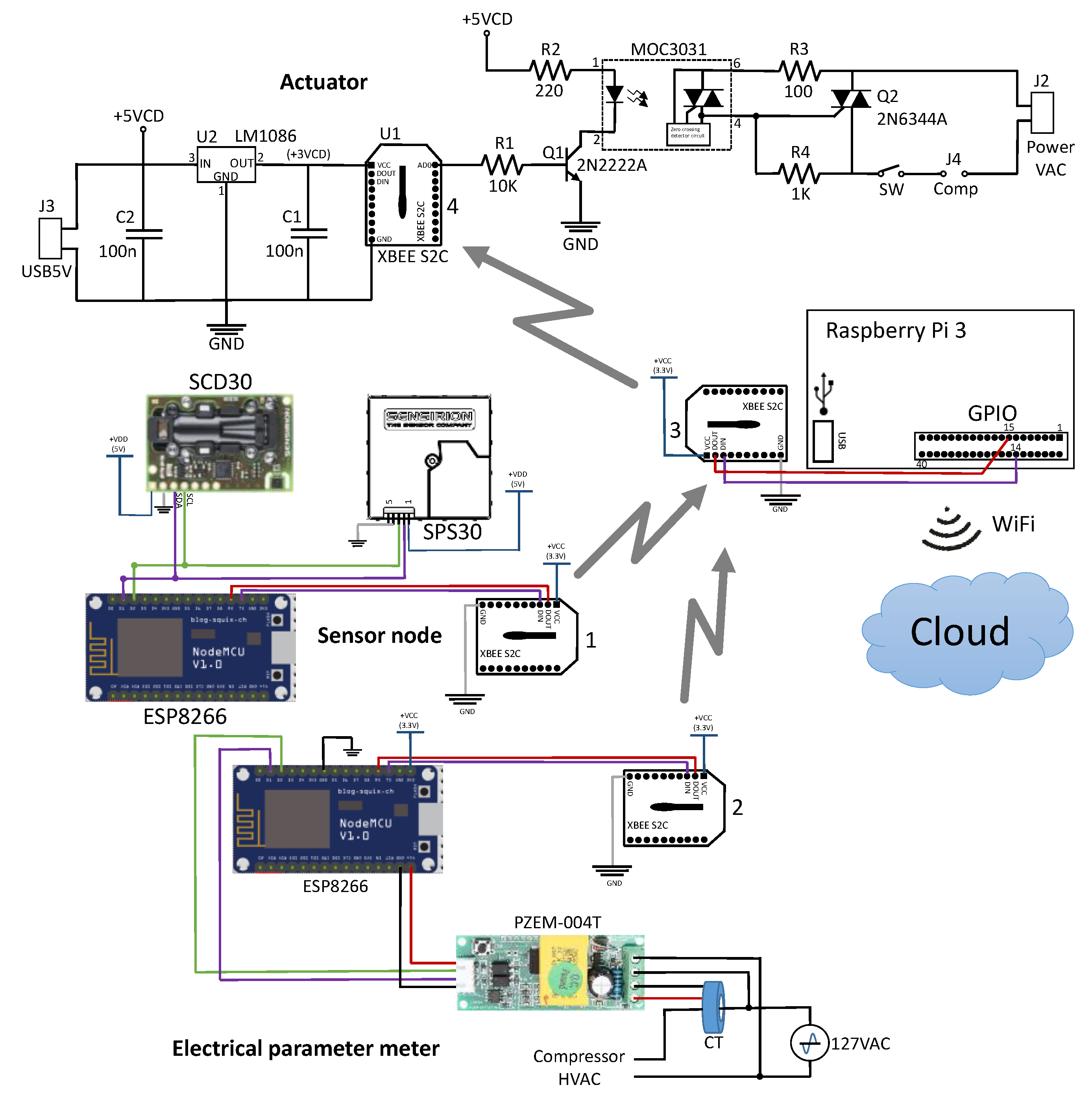
The sensor node was developed to measure relative humidity, temperature, carbon dioxide, particulate matter 2.5 and, particulate matter 10. Temperature and relative humidity values are used to establish a thermal zone, and both are used to control the HVAC equipment. Figure 1 shows a schematic diagram for the control system.

3.1. Sensor Node

A NodeMCU ESP8266 based sensor node was developed to gather measurements of the environment variables. It included a Sensirion model SPS30 particulate material sensor and a Sensirion model SCD30 carbon dioxide, temperature, and humidity sensor. In addition, since the sensor network does not rely on Wi-Fi, a ZigBee network was used to implement the wireless communication to the control system. An XBee module was selected for this purpose. Figure 2 shows the developed circuit.

A Python program was developed to receive and store the values of the environmental variables, temperature, humidity, carbon dioxide, particulate matter 2.5 and 10, with the ability to communicate the sensor node via wireless with the Raspberry Pi. The sensor node is connected via serial with an XBee and the data of the variables is sent to the Raspberry Pi, which has another XBee connected via serial to receive the information from the sensor node wirelessly.

3.2. Electrical Meter

An electronic device created for that specific purpose, the PZEM-004T, was used to measure the electrical parameters. The PZEM-004T module is connected using its serial channel to a NodeMCU ESP8266. A program in the NodeMCU ESP8266 is used to read the data from the PZEM-004T module and then wirelessly transmitted to the Raspberry Pi using an XBee communications module. The PZEM-004T measures voltage, current, power, frequency, power factor, and power consumption. The electrical meter module is used to measure the performance of the HVAC equipment. Figure 3 shows the interconnection of the circuits used.

3.3. Actuator

An actuator module was designed to control the turning on/off of the HVAC equipment. A solid-state relay was built using an 8 amp TRIAC 2N6344A. The circuit has an XBee module to communicate wirelessly with the Raspberry Pi. The solid-state relay receives an instruction from the Raspberry Pi to turn on (full power) or off (null power) the HVAC compressor via wireless through XBee modules. Figure 4 shows the circuit implemented for the actuator.

3.4. Control System Integration

The complete system is implemented by connecting the sensor node, the electrical meter, and the actuator node with the Raspberry Pi, as shown in Figure 5.

The Raspberry Pi in the control node is connected to the cloud via Wi-Fi. The complete Python program gathers the measurements of the nodes mentioned above by sending reading commands through the XBee module connected to the serial port of the Raspberry Pi. Then the Raspberry Pi receives the measurements, stores them in a file, and decomposes the string into each of the data used. The data gathered is sent to the cloud to be stored and further processed in the ThinkSpeak platform.

Using Equations (10)–(17), a Python program was developed to calculate the PMV index, Equations (3)–(8) were also incorporated into the program. Equation (18) was used for the estimation of the PPD index.

The ambient temperature and mean radiant temperature values, t_a and t_r, respectively, are assigned using the value corresponding to the output dry bulb temperature from the sensor node. The external work variable W, according to ISO 7730, is usually considered around zero, so W = 0. The relative humidity RH comes from the sensor node. Then, only three values are required to calculate the indices, the insulation value of the clothing i_cl in clo. units, the metabolic rate M in met. units, and the relative v_ar air velocity in meters per second.

For PMV index calculation, four environmental variables are needed: ambient temperature, relative humidity, mean radiant temperature, and air velocity. Also, two individual parameters are required: the metabolic rate and the cloth index.

The HVAC control system was tested in the City of Hermosillo in summer with outdoor temperatures above 45 °C (around 113 °F). In this case, the value of 0.5 clo. is used. The metabolic rate is assumed to be 1.1 met as recommended by the ASHRAE standard [26] for office work. The air velocity is assumed to be 0.1 m/s as recommended by ASHRAE [26] for office and school spaces.

According to ASHRAE [26], dry bulb temperature can be used to approximate the operating temperature (average of dry bulb temperature and mean radiant temperature) under certain conditions. These conditions are: (1) there is no radiation from radiant panel heating and/or cooling systems, (2) if the U-factor outside the windows and walls is less than 50 (the internal design temperature minus the external temperature design), (3) the solar heat gain coefficients in the windows is less than 0.48, and (4) there is no equipment that generates extreme heat in the space. Additionally, in previous work [1,28,31], ambient temperature has been used as an approximation of the mean radiant temperature, for this control, mean radiant temperature is assumed to be equal to ambient temperature.

With all the previous assumptions, the calculation of the PMV index is simplified, so only the values of the ambient temperature and the relative humidity are required.

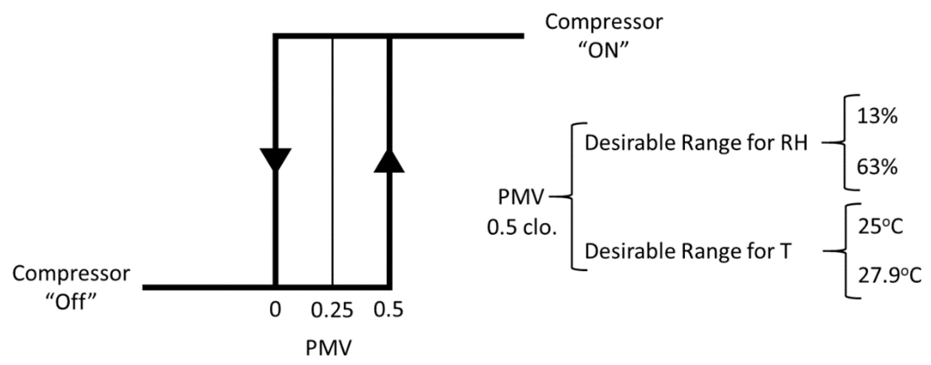
The temperature and relative humidity values gathered from the sensor node are used to locate the HVAC equipment’s operating point. With these data, the PMV and PPD indices are calculated and used to control the on and off of the HVAC equipment. The PMV value must be between 0 and 0.5 for 0.5 clo. Clothing and this parameter is set as the hysteresis window for the control system, and the setpoint value must be set to 0.25, i.e., controlling the compressor by turning it on and off in the range of 0 to 0.5. According to ASHRAE [26], in this range of PMV, the desirable range for relative humidity and temperature are 13% to 63%, and 25 °C to 27.9 °C, minimum and maximum, respectively. Figure 6 shows the comfort zones recommended by ASHRAE for 0.5 clo. And 1.0 clo. Figure 7 shows the control zone of the proposed control system. Figure 8 shows the setpoint for the HVAC compressor.

The Raspberry Pi also has a subroutine to send the data to the cloud, specifically to the ThinkSpeak platform. This platform can store all the data and, later, it can be downloaded for analysis purposes.

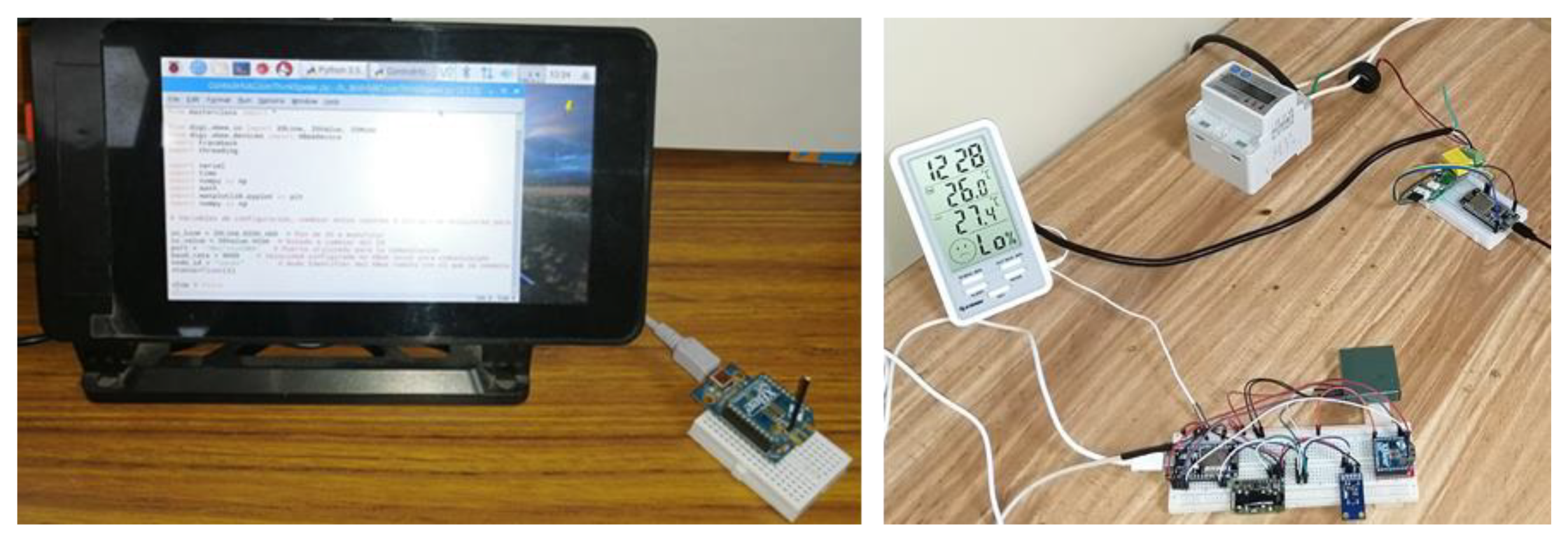
Figure 9 shows the Raspberry Pi used to control the operation of the HVAC compressor, developed sensor node and, the electrical parameter meter. Figure 10 shows the actuator installed in the HVAC equipment.

The proposed control system is programmable. Some variables could be adjusted manually in the software. These variables are air velocity, mean radiant temperature, metabolic rate, and cloth index.

4. HVAC Control System Testing

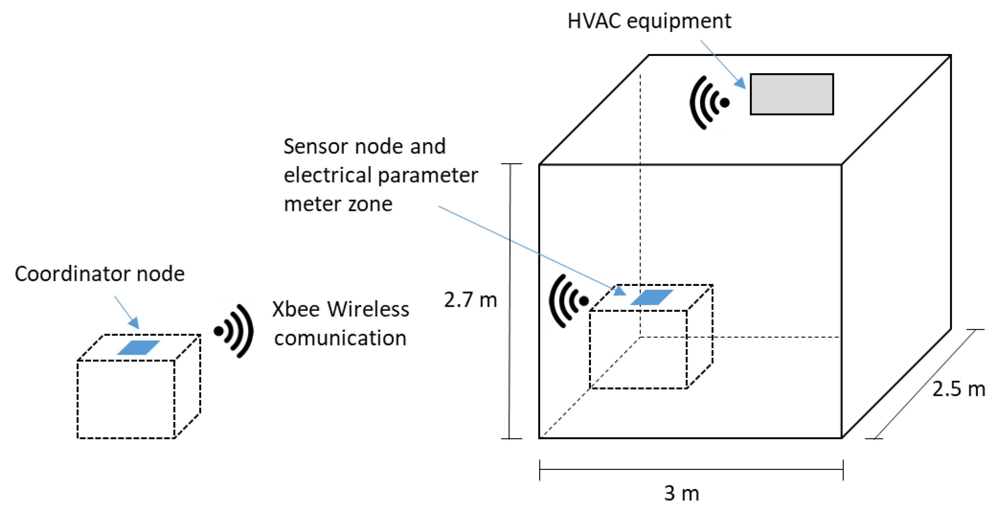
In order to test the HVAC control system, a test room has been set to install the HVAC equipment and start its operation. The test room was built inside the Electronics Laboratory of the Tecnológico Nacional de México campus Hermosillo. The room dimensions are 2.5 m wide by 3 m long, with a height of 2.7 m. A 5000 BTU Mirage Air Conditioner equipment model MACC0511N, with 115VAC supply voltage and an average consumption of 460 watts was installed in the test room. Figure 11 shows the schema of the test room. The air conditioner equipment has a standard built-in temperature-based on–off hysteresis control. The air conditioner equipment can reach a power consumption of 460 watts maximum when the compressor is turned on, and, when the compressor is turned off, the power consumption depends on the fan motor. The manufacturer does not provide information about the internal operation of the built-in control.

The built-in control is a temperature-based traditional hysteresis control, and the proposed control is a PMV-based hysteresis control. The proposed control performs the calculations of the setpoint based upon the methodology firstly proposed by Fanger combined with a digital psychometric chart to evaluate the control zone.

To perform the test for the control system, the solid-state relay was installed in the HVAC equipment in the power input of the compressor. With the actuator connected to the HVAC equipment, it is possible to control the compressor operation and outlet air temperature remotely. This control system has been developed for the air conditioning operation.

The HVAC equipment control system can remotely control the compressor on and off through the XBee modules installed in the Raspberry Pi and the actuator. The sensor node measures the values of the environmental variables and sends the information obtained to the Raspberry Pi through the Xbee modules. The same goes for the electrical meter; it collects the measurements and sends them to the Raspberry Pi.

4.1. Data Collection

The Raspberry Pi node collects the measurement data from the sensor node and the electrical meter and sends it to the cloud to the ThinkSpeak platform. In addition, the calculation of the setpoint for the HVAC equipment is performed using the temperature and relative humidity measurements sent by the sensor node, this calculation is used to turn on and off the HVAC compressor. The calculation of the setpoint is also associated with the value of the PMV index.

Operational tests have been performed on the test room, using the proposed HVAC control and the HVAC built-in control. All the measurements, the built-in control, and the proposed control are stored on the ThinkSpeak platform. These measurements are a total of 107.124 records on electrical parameters and 50.233 records on environmental variables.

4.2. Sample Size

To allow comparison between the built-in HVAC control system and the proposed control system, the HVAC equipment in the test room was operated with both control systems. Several tests were performed to measure environmental variables and electric variables on different days and at different hours in order to characterize the power consumption of the HVAC and to make a comparison. To find the sample size required to ensure an acceptable level of reliability for the mean value of the measurements, an initial pre-sample size of 10 was set [32].

Table 4. Sample of power consumption of the HVAC equipment with the built-in and the proposed control system.

	Built-in Control System		Proposed Control System
Sample	Power Consumption (Wh)	Average Temperature Setpoint (°C)	Power Consumption (Wh)	Average Temperature Setpoint (°C)
1	236.20	25.03	119.91	26.63
2	238.38	25.09	122.45	26.60
3	240.78	24.91	119.78	26.73
4	240.62	24.96	120.41	26.66
5	238.05	24.96	123.07	26.65
6	237.34	24.80	124.06	26.62
7	238.99	24.95	122.96	26.80
8	239.93	24.98	126.84	26.89
9	241.59	24.84	123.33	26.69
10	243.44	24.47	122.07	26.83

shows the power consumption of the HVAC equipment with the built-in and proposed control systems, and the average temperature setpoint value for each control system.

With the 10-size pre-sample of power consumption for both control systems, the next step is to calculate the sample size required to ensure stable power consumption values and that they are representative of the population. In order to calculate the sample size, it is necessary to calculate the mean and standard deviation of the pre-sample. For the pre-sample of the built-in control,

$$\overline{x_1}=\frac{{{\displaystyle \sum }}_{i=1}^n{x}_i}{n}=\frac{2395.0}{10}=239.53$$

(19)

$$S_1=\sqrt[2]{\frac{{{\displaystyle \sum }}_{I=1}^n{\left(x_i-\overline{x}\right)}^2}{n-1}}=\sqrt[2]{\frac{42.13}{10-1}}=2.16$$

(20)

and for the pre-sample of the proposed control system,

$$\overline{x_2}=\frac{{{\displaystyle \sum }}_{i=1}^n{x}_i}{n}=\frac{1224.88}{10}=122.49$$

(21)

$$S_2=\sqrt[2]{\frac{{{\displaystyle \sum }}_{I=1}^n{\left(x_i-\overline{x}\right)}^2}{n-1}}=\sqrt[2]{\frac{42.23}{10-1}}=2.14$$

(22)

With the mean and standard deviation values of both pre-samples [33], the sample size is calculated to ensure that the power consumption variable stabilizes in both controls using,

$$n_x={\left(\frac{S·t_{\alpha /2,n-1}}{\in }\right)}^2$$

(23)

where n_x is the sample size that ensures that the energy consumption variable stabilizes with a confidence level of 1 − α, α is the rejection level, t_α/2,n−1 is the value corresponding to that rejection level α with that value of the sample size in the table corresponding to the t-student distribution. The parameter “∈” is the degree of accuracy for the variation between parameter measurements to be considered.

In the case of α, this value is set at 5%, i.e., with 100 measurements of the average power performed, only 5 of them would be out of the desired accuracy. The parameter t_α/2,n−1 is evaluated for α selected, and with the size of the pre-sample taken as 10, the parameter would be t_0.025,9, and the result value is obtained from the table of critical values for the t-student distribution. The parameter ∈ is considered to be 1, this means a maximum error of one watt is allowed in the measurement of the average power consumption.

So, for α = 0.05, from the t-student table, a value of t_0.025,9 = 2.262 is obtained, and using the results of (19) and (20) in (23), the sample size for the built-in control is

$$n_1={\left(\frac{\left(2.16\right)·\left(2.262\right)}{1}\right)}^2=23.95$$

(24)

and, from (21) and (22) in (23), the sample size for the proposed control is

$$n_2={\left(\frac{\left(2.14\right)·\left(2.262\right)}{1}\right)}^2=23.43$$

(25)

To ensure that the value of the average power consumption is located in the sample, it is necessary to obtain samples of the power consumptions of both control systems with values of n₁ of 24 and n₂ of 24. These values are required for an error of one watt, and 95% of an acceptable level. n₁ represents the sample-size related to the HVAC equipment’s built-in control and n₂ represents the sample related to the proposed control.

4.3. Tests Descriptions

Three different experiments were designed and carried out to test the proposed control system’s energy savings. The first experiment performed was designed to measure the base-line power consumption of the HVAC equipment with its built-in control system and default settings. The second experiment measured the power consumption of the HVAC with the proposed control system using its self-calculated setpoint. The last experiment was designed to gather the HVAC operating performance measurements with a temperature setpoint of the built-in control set to match the average temperature obtained with the proposed control. The goal of this test was to perform a comparison of the energy consumption under the same operating temperature. Each test gathers information of 30 h of HVAC equipment operation.

The HVAC equipment was installed in the test room and the measurements were obtained. To analyze the HVAC equipment power consumption, 30 samples at a 1- sample/hour rate were taken with both control systems to calculate the mean and standard deviation of the population of each control, with a rejection level of 5%, and an error of 1 watt. The sample hour was taken in different days and hours.

5. Results and Discussion

The tests described in Section 4.3 were performed.

Table 5. Power consumption, temperature, and humidity of the HVAC equipment with the built-in control system.

Index	Sample Day (Hour)	Average Power Consumption (Wh)	Average Temperature (°C)	Average Relative Humidity (%)
1	17 November 2020 (11–12)	228.59	25.00	32.75
2	17 November 2020 (13–14)	236.20	25.03	33.32
3	17 November 2020 (14–15)	238.38	25.09	32.94
4	18 November 2020 (13–14)	220.92	24.89	30.63
5	18 November 2020 (14–15)	240.78	24.91	30.56
6	18 November 2020 (15–16)	235.11	24.92	30.50
7	18 November 2020 (16–17)	240.62	24.96	30.30
8	18 November 2020 (17–18)	244.87	24.97	30.04
9	18 November 2020 (18–19)	238.05	24.96	29.98
10	18 November 2020 (19–20)	236.80	24.96	30.20
11	18 November 2020 (20–21)	239.39	24.93	30.50
12	19 November 2020 (10–11)	233.71	24.89	33.46
13	19 November 2020 (11–12)	237.34	24.80	36.16
14	19 November 2020 (12–13)	236.99	24.97	34.77
15	19 November 2020 (13–14)	238.99	24.95	34.51
16	19 November 2020 (14–15)	246.84	24.96	34.54
17	19 November 2020 (15–16)	265.02	25.01	34.46
18	19 November 2020 (16–17)	251.69	25.06	34.43
19	19 November 2020 (17–18)	259.16	25.07	34.57
20	19 November 2020 (18–19)	265.09	25.01	34.70
21	19 November 2020 (19–20)	239.93	24.98	35.05
22	19 November 2020 (20–21)	238.78	24.98	35.34
23	20 November 2020 (10–11)	233.42	24.71	42.40
24	20 November 2020 (11–12)	217.46	24.79	42.54
25	20 November 2020 (12–13)	241.59	24.84	42.97
26	20 November 2020 (13–14)	241.46	24.79	44.59
27	20 November 2020 (14–15)	240.25	24.68	45.74
28	20 November 2020 (15–16)	221.94	24.44	47.97
29	20 November 2020 (16–17)	236.40	24.38	48.61
30	20 November 2020 (17–18)	243.44	24.47	47.88
	Total	7189.20
	Avg.	239.94	24.88	36.21
	(KWh)	7.19

and

Table 6. Power consumption, temperature. and humidity of the HVAC equipment with the proposed control system.

Index	Sample Day (Hour)	Average Power Consumption (Wh)	Average Temperature (°C)	Average Relative Humidity (%)
1	23 November 2020 (14–15)	119.91	26.63	38.90
2	23 November 2020 (15–16)	139.72	26.63	37.79
3	23 November 2020 (16–17)	122.45	26.60	36.85
4	23 November 2020 (17–18)	119.78	26.73	35.94
5	24 November 2020 (13–14)	126.59	26.67	35.57
6	24 November 2020 (14–15)	120.41	26.66	35.86
7	24 November 2020 (15–16)	128.39	26.65	36.18
8	24 November 2020 (16–17)	126.84	26.54	37.25
9	24 November 2020 (17–18)	123.07	26.65	37.58
10	24 November 2020 (18–19)	124.06	26.62	37.83
11	25 November 2020 (9–10)	122.96	26.80	30.36
12	25 November 2020 (10–11)	142.36	26.77	30.91
13	25 November 2020 (11–12)	151.65	26.76	31.12
14	25 November 2020 (12–13)	146.81	26.71	32.17
15	25 November 2020 (13–14)	155.69	26.67	32.63
16	25 November 2020 (14–15)	171.35	26.65	32.66
17	25 November 2020 (15–16)	164.75	26.69	33.06
18	26 November 2020 (12–13)	133.27	26.75	30.84
19	26 November 2020 (13–14)	126.84	26.89	30.41
20	26 November 2020 (14–15)	131.61	26.78	30.40
21	26 November 2020 (15–16)	137.25	26.81	30.06
22	26 November 2020 (16–17)	141.87	26.81	29.83
23	26 November 2020 (17–18)	147.17	26.76	30.17
24	26 November 2020 (18–19)	126.62	26.85	30.57
25	26 November 2020 (19–20)	132.70	26.82	31.01
26	27 November 2020 (11–12)	134.27	26.69	33.03
27	27 November 2020 (13–14)	123.33	26.69	34.86
28	27 November 2020 (15–16)	129.67	26.68	35.14
29	27 November 2020 (17–18)	119.42	26.72	33.82
30	27 November 2020 (18–19)	122.07	26.83	32.86
	Total	4012.88
	Avg.	133.76	26.72	33.52
	(KWh)	4.01

show the power consumption of the HVAC equipment with the built-in and proposed control, respectively.

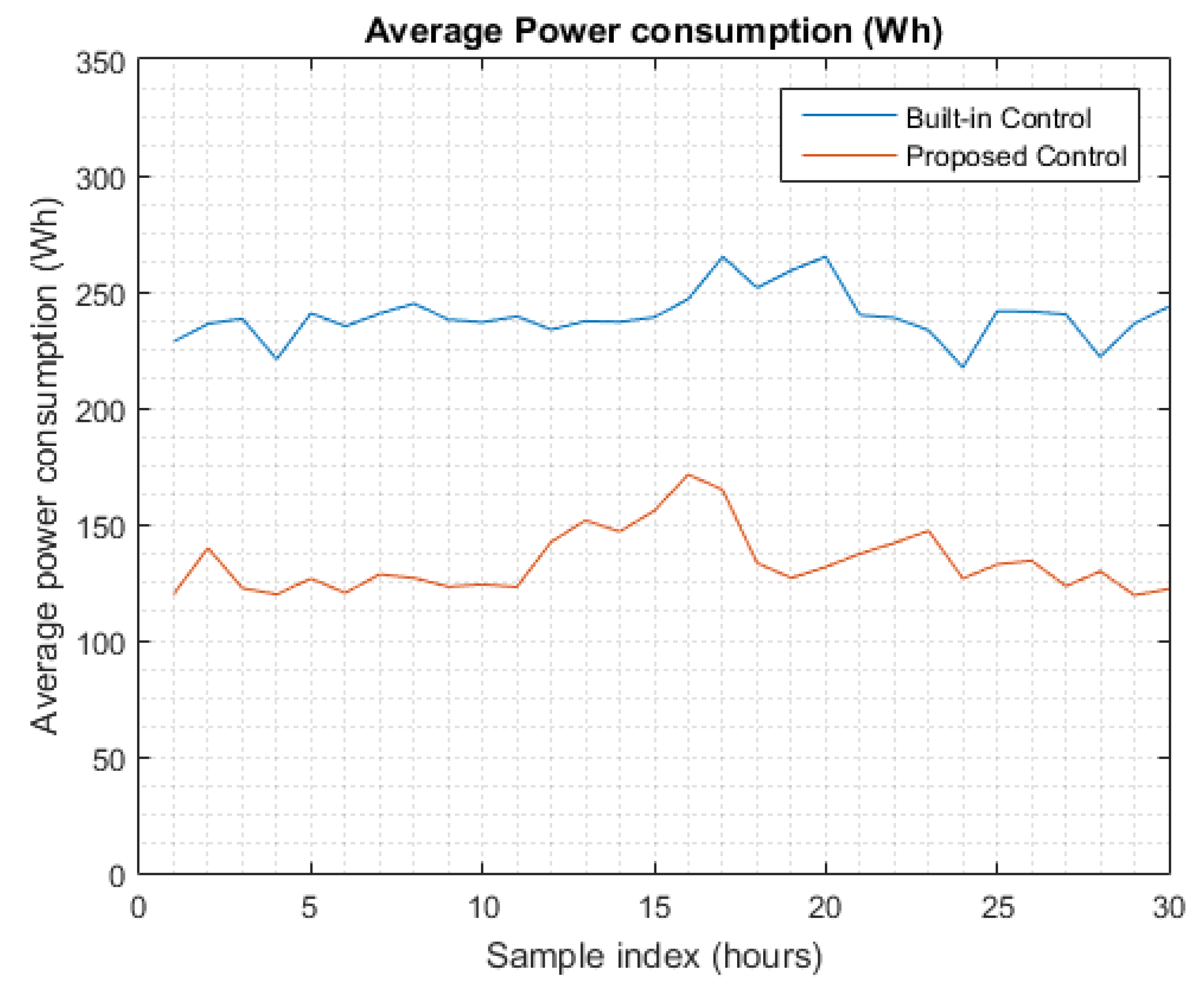
Figure 12 and Figure 13 show the behavior of the average power consumption and temperature for both control systems.

Figure 14 shows the behavior of the PMV index for the 30 working hours, with a total of 5355 samples. The PMV index went form a −0.117 minimum value, to 0.528 maximum value and, 0.282 average value. The proposed control calculated PMV index values within the 0 to 0.5 range and, an average value of 0.25. In addition, Figure 15 shows a comparison between the power consumption and PMV index value for one hour of operation of the HVAC equipment, in this case, 25 November 2020, from 12:00 to 13:00 h was selected. During the one-hour operation, three samples per minute were taken, for a total of 180 samples. 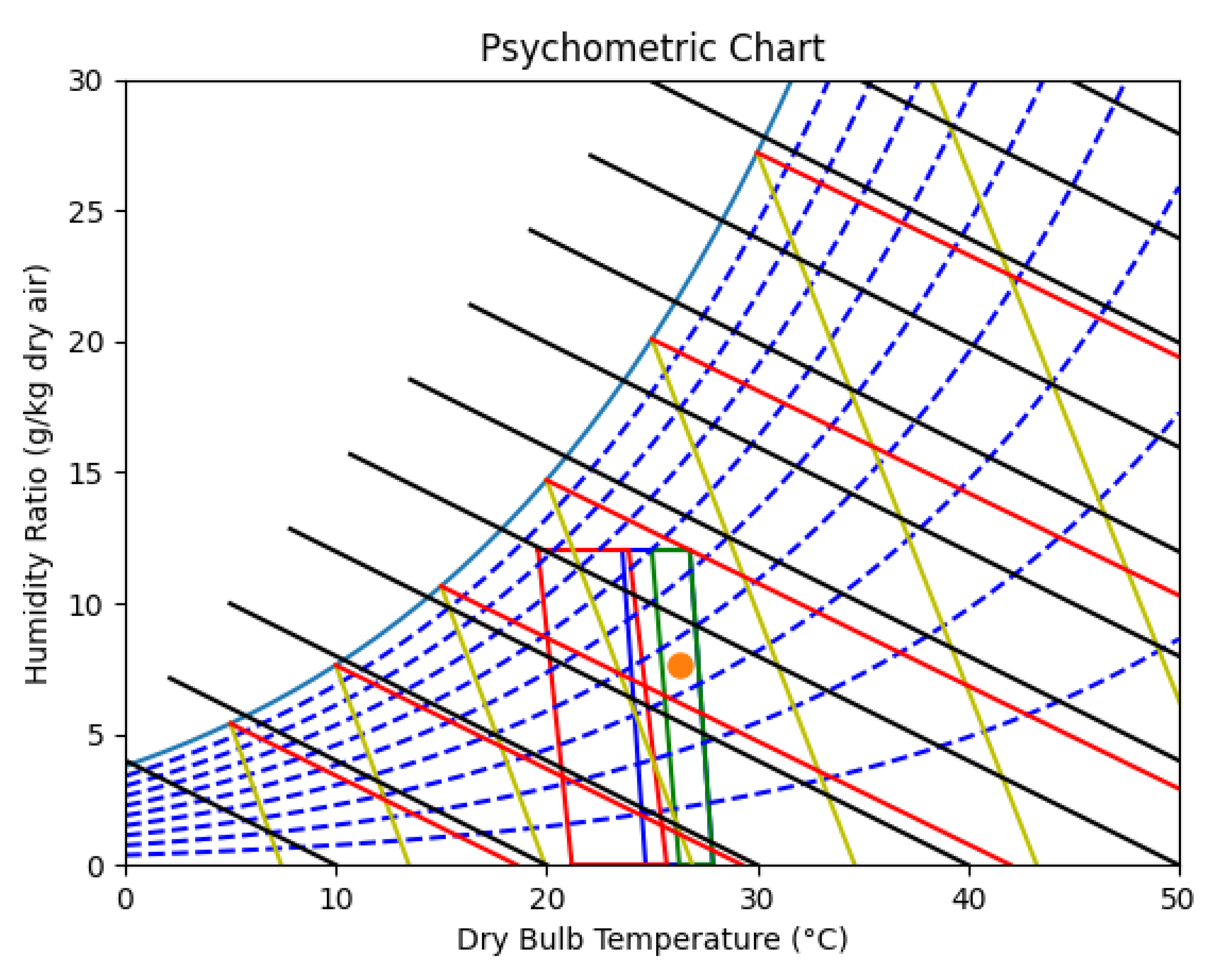Figure 16 shows the psychometric chart visualization program output. The operating setpoint (orange dot) is shown for every measurement cycle in this chart. Moreover, the green rectangle in Figure 16 represents the control zone.

Table 5 and Table 6 show the change in the average power consumption of the two control systems. Power consumption goes from 239.4 Wh with the built-in control system to 133.76 Wh with the proposed control system. The average hourly savings in power consumption by changing the HVAC equipment control is 44.18%.

In addition, the average operating temperature in the test room using the built-in control system for HVAC equipment was 24.88 °C, while with the proposed control system it was 26.72 °C. The average relative humidity was 36.21% with the built-in control system and was 33.52% with the proposed control system. The average temperature value in the proposed control system is higher than the built-in control, but this value is inside the comfort zone recommended for ASHRAE.

Thus, it can be concluded that with 95% acceptance and an error of 1 watt between the sample mean and the population mean, that the proposed HVAC equipment control system that involves the use of the PMV method to the calculation of comfort zones generates a savings of 44% in energy consumption.

The first experiment of HVAC energy consumption with the built-in control system was performed with the default values of the HVAC equipment. A second experiment of HVAC energy consumption was performed by trying to reach (with the built-in control system) the same operating temperature used in the proposed control system. These measurements are shown in

Table 7. Power consumption, temperature, and humidity of the HVAC equipment with the built-in control system with average operating temperature of 26.58 °C.

Index	Sample Day (Hour)	Average Power Consumption (Wh)	Average Temperature (°C)	Average Relative Humidity (%)
1	07 September 2021 (11–12)	308.10	27.08	42.12
2	07 September 2021 (17–18)	156.70	25.87	50.27
3	08 September 2021 (8–9)	229.99	28.97	39.83
4	08 September 2021 (9–10)	205.36	28.48	38.82
5	08 September 2021 (10–11)	185.00	28.19	38.41
6	08 September 2021 (11–12)	140.97	26.54	41.45
7	08 September 2021 (12–13)	128.21	26.57	42.38
8	08 September 2021 (13–14)	129.58	26.46	43.31
9	08 September 2021 (14–15)	200.78	26.29	48.32
10	08 September 2021 (15–16)	223.21	26.53	49.74
11	08 September 2021 (16–17)	256.70	26.88	51.48
12	09 September 2021 (10–11)	278.50	26.09	43.65
13	10 September 2021 (9–10)	63.35	26.13	43.30
14	10 September 2021 (10–11)	62.87	26.37	44.61
15	10 September 2021 (11–12)	147.20	25.89	44.86
16	10 September 2021 (15–16)	240.77	26.18	50.44
17	10 September 2021 (16–17)	259.12	26.56	49.62
18	10 September 2021 (17–18)	294.14	26.70	48.53
19	10 September 2021 (18–19)	332.44	26.71	47.49
20	14 September 2021 (11–12)	163.97	26.14	53.45
21	14 September 2021 (12–13)	149.18	26.02	51.96
22	14 September 2021 (13–14)	181.03	26.04	52.10
23	14 September 2021 (14–15)	214.99	26.41	53.45
24	14 September 2021 (15–16)	283.62	26.67	51.39
25	15 September 2021 (11–12)	180.99	26.01	49.51
26	15 September 2021 (12–13)	135.97	26.06	49.47
27	15 September 2021 (13–14)	154.78	25.96	48.12
28	15 September 2021 (14–15)	211.25	26.20	50.07
29	15 September 2021 (15–16)	256.06	26.58	51.30
30	15 September 2021 (16–17)	298.42	26.70	49.85
	Total	6073.25
	Avg.	202.44	26.58	47.31
	(KWh)	6.07

.

Figure 17 and Figure 18 show the average power consumption and temperature behavior with the proposed and built-in control system with 26.58 °C. In Figure 17, the average power consumption shows a varying behavior due to the operation of the built-in hysteresis control of the HVAC equipment. For example, in the sample hours 13 and 14, the average power consumption depended only on the fan motor, i.e., the compressor was off for the whole hour. On the other hand, when the built-in control works with the default settings, its operation is smoother (Figure 12).

Table 6 and Table 7 show the change in the average power consumption of the two control systems taking into account the nearest operating average temperature. Power consumption goes from 202.4 Wh with the built-in control system to 133.76 Wh with the proposed control system. The average hourly savings in power consumption by changing the HVAC equipment control was 33.9%.

Furthermore, the average operating temperature in the test room using the built-in control system for HVAC equipment was 26.58 °C, while with the proposed control system it was 26.72 °C. The average relative humidity was 47.31% with the built-in control system and was 33.52% with the proposed control system. The difference in average operating temperature between the two control systems is negligible.

Thus, it can be concluded that with 95% acceptance and an error of 1 watt between the sample mean and the population mean, that the proposed HVAC equipment control system that involves the use of the PMV method to the calculation for comfort zones generates savings among 33% to 44% in energy consumption compared with the built-in control that uses a typical temperature-based on–off hysteresis control. Further testing is required to draw energy-saving conclusions over an inverter type controller.

Other PMV-based controls obtained different energy savings depending on the environmental conditions of the tests performed in each case. The PMV-PPD-based control presented in [25] reported energy savings up to 11.5% compared to a traditional temperature-based thermostat. This control works with a fixed setpoint using a PPD index selected by the occupants. The PMV value is the control signal for the HVAC compressor.

The automatic temperature setpoint PMV-based control system presented in [27] reports an energy savings of 13.6% and 14.6% for a typical summer day.

The comparative Computational Fluids Dynamics (CFD) simulation study presented in [23] reports savings of 1.6% per day of energy consumption. The simulation was conducted in a typical glazed office room subjected to solar radiation for an occupied typical summer day.

The thermal comfort-based (PMV-based) control presented in [1] reports an average of 33.5% of energy savings. However, in a representative day in the summer season, it reports 39.5% of energy savings.

The PMV-based control system presented in [28] reports experimental results of energy saving of 34.7%, 37.3%, and 32.9%, using an inverse PMV model with feedforward PID control, an inverse PMV model with feedforward fuzzy control, and an inverse PMV model with self-turning control, respectively.

The proposed PMV-based control system was tested in the summer season with outdoor temperatures above 45 °C (around 113 °F). The achieved energy savings of 33% to 44% are consistent with the results obtained with the PMV-based control model and similar environmental test conditions.

The proposed PMV-based control uses the ambient temperature value as the mean radiant temperature, but the adjusting capability (via programming) of the proposed control system can use an environmental sensor of mean radiant temperature. Moreover, it is possible to estimate the mean radiant temperature values using any of the calculation techniques available.

This PMV-based control can be used in other HVAC equipment, not only the one reported here. With a slight modification in the solid-state switch power handling capability, the proposed control can be used with other HVAC equipment.

6. Conclusions

This paper presented an alternative control system to reduce energy consumption in HVAC equipment. The proposed control system is based upon the PMV index and, it controls the operation of the HVAC equipment via wireless XBee modules. The control hardware is composed of a sensor node, an electrical parameter meter, a solid-state actuator, and a coordinator node. The coordinator node collects the measured data from the sensor node and the electrical parameter meter and sends it to the ThinkSpeak platform. Additionally, the setpoint to control the HVAC equipment is calculated using the sensor node’s temperature and relative humidity measurements based upon the PMV index.

The average power consumption with the built-in control system decreases from 239.4 Wh down to 133.76 Wh with the proposed control system. This represents an average savings of 44.18% in power consumption of the HVAC equipment by replacing the built-in control with the proposed one. This is achieved with an error of only one watt, and a 95% acceptance. Additionally, reaching the average operating temperature in the test room using the built-in control system for HVAC equipment and comparing it with the data obtained for the proposed control system is possible to achieve a 33.9% of energy savings. Thus, the proposed HVAC equipment control system that involves the use of the PMV method for the calculation of comfort zones generates savings ranging from 33% to 44% in energy consumption using a control zone of 0 to 0.5 PMV index value. Other PMV-based controls report energy savings in the range from 13.6 to 39.5% with similar operating conditions.

In summary, the proposed control system, incorporating the PMV and PPD indexes to calculate the temperature setpoint along with the relative humidity value improves the BEMS control of an HVAC equipment. The proposed control for the HVAC equipment achieves an energy savings without compromising user comfort. The energy saving can be seen as a reduction in the energy generated by the utility, and this could be seen as a reduction in greenhouse emissions as a result of the unburned fuel, helping to mitigate the effects of climate change. Although the implementation of the proposed control system includes additional elements that increase the cost of the equipment, important advantages are achieved, such as the reduction in energy consumption and the control of the equipment remotely. In addition, the additional cost is amortized in the short term by savings in energy consumption.

Future work to reduce energy consumption in the HVAC system can include setpoints changes depending on the number of users present, and the availability of use of the space. A detailed analysis of the data collected and stored in the cloud can also be performed; the data related to environmental variables can be analyzed to detect possible trends and make forecasts, and the data related to electrical measurements, in addition to trends and forecasts, can be analyzed to detect potential future failures [34] or equipment maintenance trends. Another interesting research path to be explored is to include efficient predictive controllers, as those reported in [35,36,37], that have been tested on embedded platforms with little processing power and storage capacity [38] in conjunction with inverted-type HVAC compressors.