
Hybrid Model for Forecasting Indoor CO2 Concentration

1
Department of Building Research, Korea Institute of Civil Engineering and Building Technology, 283 Goyangdae-ro, Ilsanseo-gu, Goyang-si 10223, Gyeonggi-do, Korea
2
Department of Building Energy Research, Korea Institute of Civil Engineering and Building Technology, 283 Goyangdae-ro, Ilsanseo-gu, Goyang-si 10223, Gyeonggi-do, Korea
3
Research Strategic Planning Department, Korea Institute of Civil Engineering and Building Technology, 283 Goyangdae-ro, Ilsanseo-gu, Goyang-si 10223, Gyeonggi-do, Korea
*
Author to whom correspondence should be addressed.
Buildings 2022, 12(10), 1540; https://0-doi-org.brum.beds.ac.uk/10.3390/buildings12101540
Submission received: 6 September 2022
/
Revised: 21 September 2022
/
Accepted: 23 September 2022
/
Published: 27 September 2022
(This article belongs to the Special Issue Modeling, Analysis, Optimization and Control of HVAC Systems in Buildings)
Abstract
:Indoor CO2 concentration is considered a metric of indoor air quality that affects the health of occupants. In this study, a hybrid model was developed for forecasting the varying indoor CO2 concentration levels in a residential apartment unit in the presence of occupants by controlling the ventilation rates of a heat recovery ventilator. In this model, the mass balance equation for a single zone as a white-box model was combined with a Bayesian neural network (BNN) as a black box model. During the learning process of the hybrid model, the BNN estimated an aggregated unknown ventilation rate and transferred the estimation to the mass-balance equation. A parametric study was conducted by changing the prediction horizons of the hybrid model from 5 to 15 min, and the forecasting performance of the hybrid model was compared with the stand-alone mass balance equation. The hybrid model showed better forecasting performance than that of the mass balance equation on the experimental dataset for a living room and bedroom. The average MBE and CVRMSE of the hybrid model for the prediction horizon of 15 min were 0.65% and 5.23%, respectively, whereas those of the mass balance equation were 0.99% and 9.30%, respectively.
1. Introduction
Buildings account for approximately 40% of the global energy consumption and 30% of global greenhouse gas emissions and are becoming one of the most energy-consuming sectors [1]. The South Korean government has announced an increase in the greenhouse gas reduction target from 26.3% to 40% of the 2018 levels by 2030 [2]. Additionally, energy-efficient building operations are key factors for implementing a 32.8% reduction in carbon emissions in the building sector, which is a crucial part of achieving carbon neutrality by 2050 [3]. Heating, ventilation, and air conditioning (HVAC) systems are responsible for the largest category of end-use energy consumption in buildings [4]. However, the energy savings of HVAC systems should not have an adverse effect on occupants’ health or welfare, since the comfort of the occupants may be negatively affected by reducing the energy used by the HVAC [5].
Indoor carbon dioxide (CO2 is considered the main indicator of indoor air quality (IAQ), which affects the health of occupants. Although no direct causal link was found between exposure to CO2 and the sick building syndrome (SBS) symptoms [6], CO2 is approximately correlated with other indoor pollutants that may cause SBS symptoms. In this regard, CO2 concentration has started to be used as a metric of ventilation by the American society of heating, refrigerating, and air-conditioning engineers (ASHRAE) standard 62 [7] in 1981 [8]. Since then, a CO2 concentration limit for the management of IAQ concerns and SBS symptoms has been commonly recommended by several standards [9,10,11].
Meanwhile, the key objective of HVAC systems’ operation is to solve the conflict between energy consumption of HVAC systems and comfort of occupants, as they typically have the opposite effects on one another [12]. In particular, considering the mass balance, the concentration of indoor pollutants emitted from indoor sources decreases as ventilation rates increase, but ventilation rates affect the energy required for heating and cooling, with higher ventilation rates generally increasing energy requirements for air-conditioned spaces [13]. Therefore, HVAC systems should be controlled to minimize the energy consumption by providing appropriate ventilation rates in accordance with varying outdoor and indoor conditions.
Model predictive control (MPC) is a promising candidate for smart buildings, efficient control, high energy savings, and improving indoor environments [14,15]. MPC uses a model to predict the future states of a system and generates a control vector that minimizes a certain cost function over the prediction horizon in the presence of disturbances and constraints [16]. Additionally, the MPC scheme has been widely used for HVAC control to improve IAQ and thermal comfort as well as achieve energy savings [5,17,18,19]. The MPC scheme consists of a prediction model, an objective function for the optimization problem, and a control law with constraints [14]. However, issues regarding the selection of an appropriate model and prediction horizon, as well as methods to handle uncertainty in system modeling and external disturbance parameters such as temperature, wind speed, solar radiation, and so on, continue to exist when implementing MPC [14].
Although the white box (also known as a physics model), black box (also known as a data-driven model or a machine learning model), and grey box (an approximation of the heat transfer mechanisms of an analogous electrical lumped resistance and capacitance networks models) have been used for MPC, the requirement for a perfect model has not yet been fulfilled [14,20]. Kallio et al. [1] studied the applicability of four machine learning models, Ridge regression, Decision Tree, Random Forest, and Multilayer Perceptron, to forecast CO2 concentrations in office rooms. Taheri and Razban [4] developed six machine learning models, Support Vector Machine, AdaBoost, Random Forest, Gradient Boosting, Logistic Regression, and Multilayer Perceptron, to forecast CO2 concentrations of a campus classroom. Compared to the existing studies, the authors introduce a hybrid model that combines the white box and black box models for forecasting CO2 concentrations. In [21], the hybrid model was suggested for achieving improved performance rather than the traditional machine learning model in terms of reliability, explainability, flexibility, and feasibility [21]. The hybrid model automatically estimates the unknown input variables of the white box model using the learning principle of an ordinary black box model, such that the physics model can be applied even if an unknown input variable exists. Ahn et al. [21] demonstrated that the prediction target of the hybrid model was the compressor power of a variable refrigerant flow (VRF) system, and the white box and black box models were VRF-SysCurve of EnergyPlus and a Bayesian neural network (BNN), respectively. The BNN in the hybrid model can quantify the aleatoric and epistemic uncertainties caused by inherent data noise and uncertainties in the model parameters, respectively [22,23]. In particular, Ahn et al. [21] conducted parametric studies for simulating the compressor power of the VRF system using standalone BNN and hybrid models. A comparison of the standalone BNN and the hybrid model showed that the hybrid model had reliable predictive performance for unseen test dataset rather than the standalone BNN.
In this study, the authors developed a hybrid model to forecast changing indoor CO2 concentrations under the control of a residential heat recovery ventilator (HRV) for application to the MPC of the HRV. A series of experiments were conducted to record the varying CO2 concentrations in a 59-m2 apartment unit, which included a living room, kitchen, and two bedrooms. The indoor CO2 concentration varies according to the presence and behavior of the occupants and is controlled by the ventilation rates of the HRV. The target spaces of the hybrid model were the living room and bedroom.
The hybrid model consists of a mass balance equation, which acts as the white box model, for determining the CO2 concentration of a single zone and a BNN, which acts as a black-box model. In particular, uncertainties exist in the mass balance equation owing to certain assumptions, such as the presence of well-mixed air, neglectable infiltration, and so on. Additionally, disregarding the airflow between multiple zones results in uncertainties. In this study, the uncertainties were aggregated and expressed as an input variable and then added to the mass balance equation. In the hybrid model, the BNN automatically estimates the aggregated uncertainties during the learning process and delivers them to the mass balance equation. In addition, the appropriate prediction horizon of the hybrid model was investigated, and the prediction performance of the hybrid model was compared with that of the standalone mass balance equation of a single-zone model.
2. Materials and Methods
2.1. Target Space and System
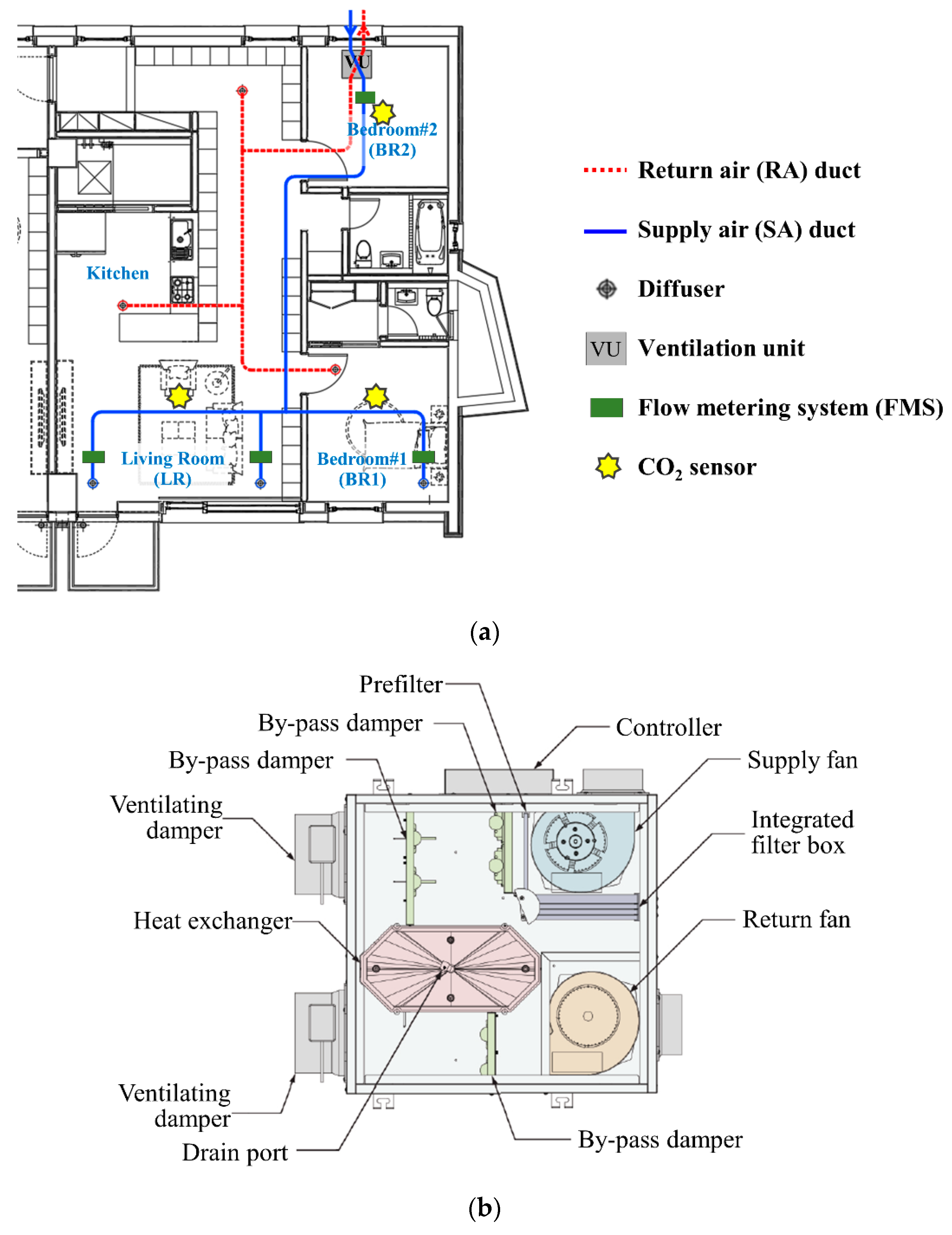
The target space is a 59 m2 apartment unit (Figure 1a), the representative size of South Korean apartments. The target space consists of a living room (LR), a kitchen, and two bedrooms (BR1 and BR2) with LR and BR1 on the southern side and BR2 on the northern side. A set of diffusers for the supply air (SA) and return air (RA) ducts were installed in BR1, and two sets of diffusers were installed in LR and the kitchen. The ventilation unit of the HRV (Figure 1b) installed in BR2 had a nominal flow rate of 150 CMH, which can support over 1 air change per hour (ACH) for a target space of 59 m2. The ventilation volume was controlled using a diffuser system with a variable air volume (VAV) (Figure 1c). The stepping motor integrated inside the diffuser cone rotated when an external controller sent operation commands to the diffuser controller via a RS 485 communication line [24]. Additionally, the ventilation volume for each room could be controlled by adjusting the speed of the SA and RA fans in the ventilation unit of the HRV and by controlling the opening rate of each diffuser.
At the end of each SA duct, the flow metering system (FMS) (Figure 1d) measured the flow rate of each room. More specifically, the FMS measured the static pressure of the duct and calculated the flow rate based on the value of the self-averaging multipitot tube [24]. The measurement tolerances of the static pressure and airflow were 1% and 2–3%, respectively. Furthermore, three EE820 CO2 sensors, which were installed 1.5 m high in the center of each space, were connected to a data logger to measure the CO2 concentration in each room (Figure 1a). The measurement range of the EE820 CO2 sensor was 0–10,000 ppm, and its tolerance was 2%.
2.2. Experiments
A total of 23 experimental cases, as listed in Table 1, were conducted twice, during which the door between LR and BR1 was alternatively closed and opened. In particular, it was assumed that the total number of occupants living in a 59-m2 apartment unit was three, and the maximum number of occupants in the LR and BR1 were set to three and two, respectively. In addition, the ventilation rate in the LR was changed to 0, 0.5, 0.7, and 1.0 ACH when the number of occupants in the LR was changed from zero to three. The number of occupants and ventilation rate in the BR1 were changed when there were no occupants in the LR. The experiments were conducted for 27 days, during which 48,430 data points that represent the CO2 concentration, number of occupants, and ventilation rate set in each diffuser were collected at 1-min intervals in LR and BR1.
3. Modeling Methods
3.1. Mass Balance Equation
The mass balance of the CO2 concentration for a mechanically ventilated zone can be expressed according to Equation (1).
where , , , , and represent the zone volume (m3), ventilation rate (m3/s), outdoor CO2 concentration (mg/m3), indoor CO2 concentration at time (mg/m3), and CO2 generation rate per person at time (mg/s), respectively. In addition, Equation (1) can be solved using Equation (2), where is the indoor CO2 concentration at time zero.
Equation (1) for a single zone is accompanied by the following assumptions: (1) the supply airflow is well-mixed with the indoor air, (2) CO2 is only diluted by ventilation, and (3) infiltration airflow and airflow between adjacent zones are negligible [8]. Additionally, the mass balance of a single zone (Equation (1)) can be adapted to multiple zones by considering the airflow between the internal zones; however, multiple unknown variables, such as the infiltration of each zone and interzonal airflow may exist [25]. In particular, the number of variables that need to be estimated may be large because the number of variables increases with the square of the number of zones [26]. For practical use in multiple zones, Federspiel [27] suggested that unknown variables should be aggregated and estimated using a first-order model.
3.2. Bayesian Neural Network
In a BNN, the uncertainty can be decomposed into aleatoric uncertainty arising from data noise and epistemic uncertainty arising from the incompleteness of the model [28,29]. Gal [30] proved that the use of the dropout technique before every weight layer with Monte Carlo (MC) sampling in a BNN can be interpreted as mathematically equivalent to the stochastic inference of the weight parameters in a neural network. In addition, Kendall and Gall [22] demonstrated that the predictive mean and variance of the model output, which is given by the predictive distribution of the BNN, can be estimated using MC sampling. Finally, the predictive mean and variance were used to decompose the predictive uncertainty into aleatoric and epistemic uncertainties [30]. The BNN is fully described in [22,28,29,30]. In this study, a BNN was used to quantify the uncertainties in forecasting indoor CO2 concentration, such that the possible uncertainties can be considered as constraints in the MPC scheme. More specifically, a BNN was used to estimate the value and quantify the uncertainties of the aggregated unknown variable of the mass balance equation in the framework of the hybrid model.
3.3. Hybrid Model
The white box model is difficult to implement in practice owing to the lack of information on its physical characteristics [31,32,33]. Additionally, the black box model suffers from poor generalization and difficulty in associating the results of the model with physical concepts [34,35,36]. Ahn et al. [21] introduced the concept of a hybrid model that combines white-box and black-box models to overcome their drawbacks. In the hybrid model, known input data are introduced into the black-box model along with parameters that have random initial values. Subsequently, the white-box model calculates the output based on the known input data and output value of the black-box model obtained using these parameters. The output of the white box model is inaccurate; however, it changes to approximate the output data of the training dataset, as the hybrid model proceeds with the learning process, to reduce the error between the output of the white box model and the output data of the training dataset. More specifically, the hybrid model automatically estimates the unknown inputs by using the learning principle of an ordinary black box model; therefore, the white box model can be applied even if an unknown input exists [21].
Ahn et al. [21] developed a hybrid model that calculates the compressor power of a VRF system based on the equations in EnergyPlus. The unknown refrigerant flow rate estimated using the BNN was used as the input variable of the equations associated with the VRF compressor power, which allowed the calculation of the compressor power based on the estimated and measured input variables.
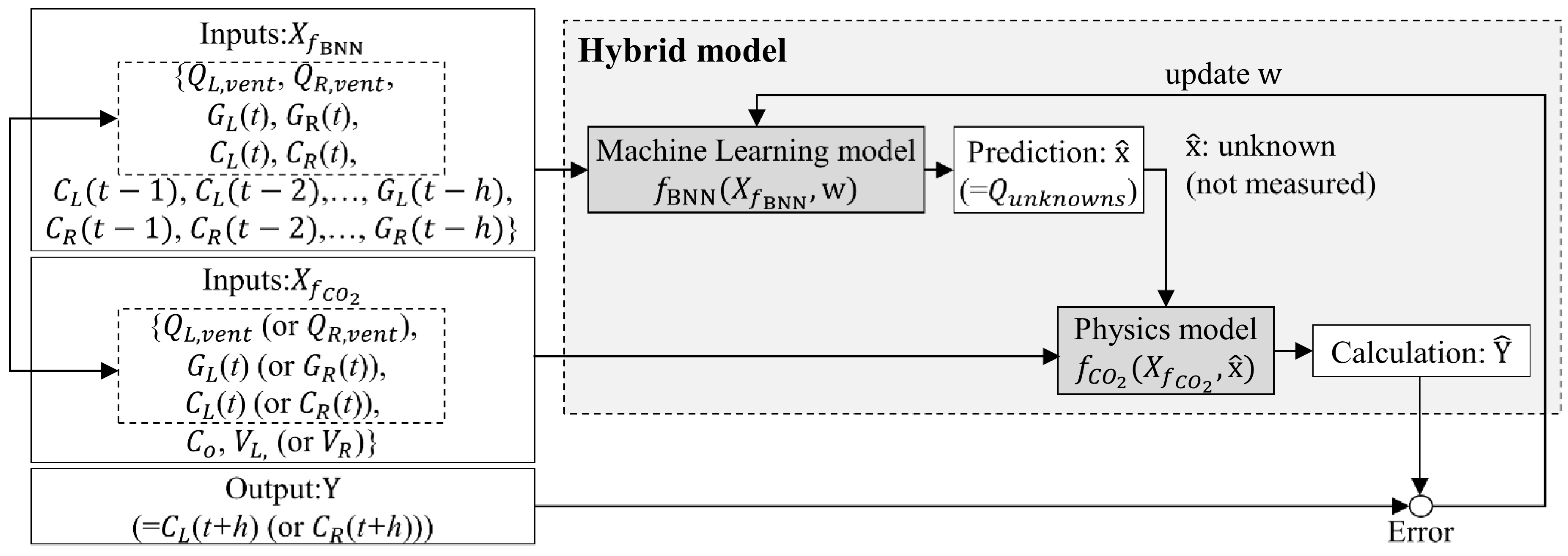
Figure 2 illustrates the concept and learning process of the hybrid model. In this study, two hybrid models were developed for forecasting the CO2 concentration in LR and BR1 (Figure 1a) under the individual ventilation control of an HRV and diffusers. The subscripts and in Figure 2 represent the LR and BR1 spaces, respectively. The white box model and black box model of the hybrid model are the mass balance equation (Section 3.1) and BNN (Section 3.2), respectively.
The ventilation rate in the mass balance equation, which refers to the outside air entering the zone, can be considered as the sum of the mechanical ventilation and infiltration [37]. Therefore, the ventilation rate term in Equations (1) and (2) was subdivided into a ventilation rate of the HRV () and an unknown ventilation rate () by considering the aggregated unknown ventilation rates, such as infiltration and interzonal airflow. Finally, Equation (3) was used as the white-box model .
For the input of , the , , and are constant values of 400 ppm, 119 m3, and 23.4 m3, respectively. In addition, , , , and are the measured values in the target space. Furthermore, and were calculated as 18 L/s per person for adult males and 16 L/s per person for adult females in accordance with ASHRAE 62.1 [38] and Korean Standard (KS) F 2603 [39]. To compute , the unknown aggregated ventilation rate must be estimated along with the known data (Figure 2) through measurements in the target space (Section 2.1). The BNN predicts the using the known data (Figure 2), including the CO2 concentrations for the past min. In contrast to , uses ventilation rates (, CO2 generation (), and CO2 concentrations (, ,…,, , ,…,) in zones LR and BR1 to consider the aggregated effects of infiltration and interzonal airflow (Figure 2).
To combine the white-box and black-box models, two activation functions were sequentially applied to a neuron in the output layer of the BNN. The first activation function was to calculate the CO2 concentration based on the estimated from the BNN, and ReLu was applied as the second activation function to prevent a negative value from being generated. In the hybrid model, the lengths of the past dataset for the input and the prediction horizon for the output were both set to (Figure 2).
4. Development of the Models
4.1. Settings Used for Model Development
In this study, the hybrid models that can forecast the indoor CO2 concentration after min over time were developed using the measured data. Two hybrid models were developed for the target zones LR and BR1. Among the 48,430 data points, including two out of the 23 experimental cases (Table 1), during which the door was closed and opened, 45,550 data points were used for training. Additionally, the remaining 2880 data points, under which two times of randomly selected six experimental cases (#1, #2, #3, #16, #17, and #18 in Table 1) when the door was closed and opened, were used for testing.
Table 2 shows the settings for the BNN used in both the hybrid models, which were determined using a trial-and-error method. Additionally, a parametric study was conducted for the prediction horizons of 5, 10, and 15 min to investigate the variation in the accuracy of the hybrid model according to the change in the prediction horizon. In addition, the results of the hybrid model were compared with the measured data and those obtained using the mass balance equation (Equation (2)). Three performance indicators, the mean bias error (MBE, Equation (4)), coefficient of variation of the root mean square error (CVRMSE, Equation (5)), and coefficient of determination (R2, Equation (6)), were selected to evaluate and compare these performances.
where is the number of data points, is the model output, is the measurement, and is the mean measurement.
4.2. Results
As mentioned in Section 3.2, the predictive uncertainty, which consists of aleatoric and epistemic uncertainties, can be provided along with the predictive mean of the BNN used in the hybrid model. Table 3 and Figure 3, Figure 4 and Figure 5 show the forecasting results obtained from the hybrid model and from the mass balance equation for the test dataset. In Figure 3, Figure 4 and Figure 5, “Hybrid predictive mean” and “Calculation” indicate the forecasting results of the hybrid model and mass balance equation, respectively. Additionally, “Aleatory” and “Epistemic” mean the aleatoric and epistemic uncertainties of the hybrid model, respectively, and Aleatory + Epistemic is the total predictive uncertainty of the hybrid model. Furthermore, “Hybrid uncertainty (upper)” and “Hybrid uncertainty (lower)” are the upper and lower boundaries, respectively, of the total predictive uncertainty of the hybrid model. In addition, the test dataset in Figure 3 and Figure 4 was divided into two sections (March 21 and 22) so that the forecasting results can be clearly identified.
As shown in Table 3, the hybrid models applied to LR and BR1 exhibit better forecasting performance than that of the mass balance equation in terms of the most performance indicators of the three prediction intervals. When the prediction horizon used for the LR zone was increased from 5 min to 15 min, the forecasting performance of the mass balance equation was degraded further than that of the hybrid model. For example, the MBE and R2 of the hybrid model showed marginal changes, whereas the MBE and R2 of the mass balance equation decreased by 1.57% (from −0.85% to −2.42%) and 0.04 (from 0.99 to 0.95), respectively. The only case that exhibited a better forecasting result from the mass balance equation than that of the hybrid model, was the MBE of the prediction horizon of 15 min for the BR1 zone. However, determining whether the overall forecasting performance of the mass balance equation is better than that of the hybrid model is difficult when the CVRMSE and R2 are considered.
As shown in Figure 3 and Figure 4, since the mass balance equation (Equation (2)) cannot reflect the unknown and/or uncertain changes in the indoor environment during the prediction horizon of the model, the corresponding forecasting results are shifted according to the prediction horizon. In contrast, the BNN in the hybrid model estimated the aggregated unknown term by learning the relationship between the current and past CO2 concentrations (, ,…,, , ,…,) and the CO2 concentration after the prediction horizon ( or ), and the estimated was reflected in the mass balance equation (Equation (3)) of the hybrid model. Owing to the presence of , which is the only difference between the models, the forecasts of the hybrid model followed the changing trend of the measurement faster than the mass balance equation.
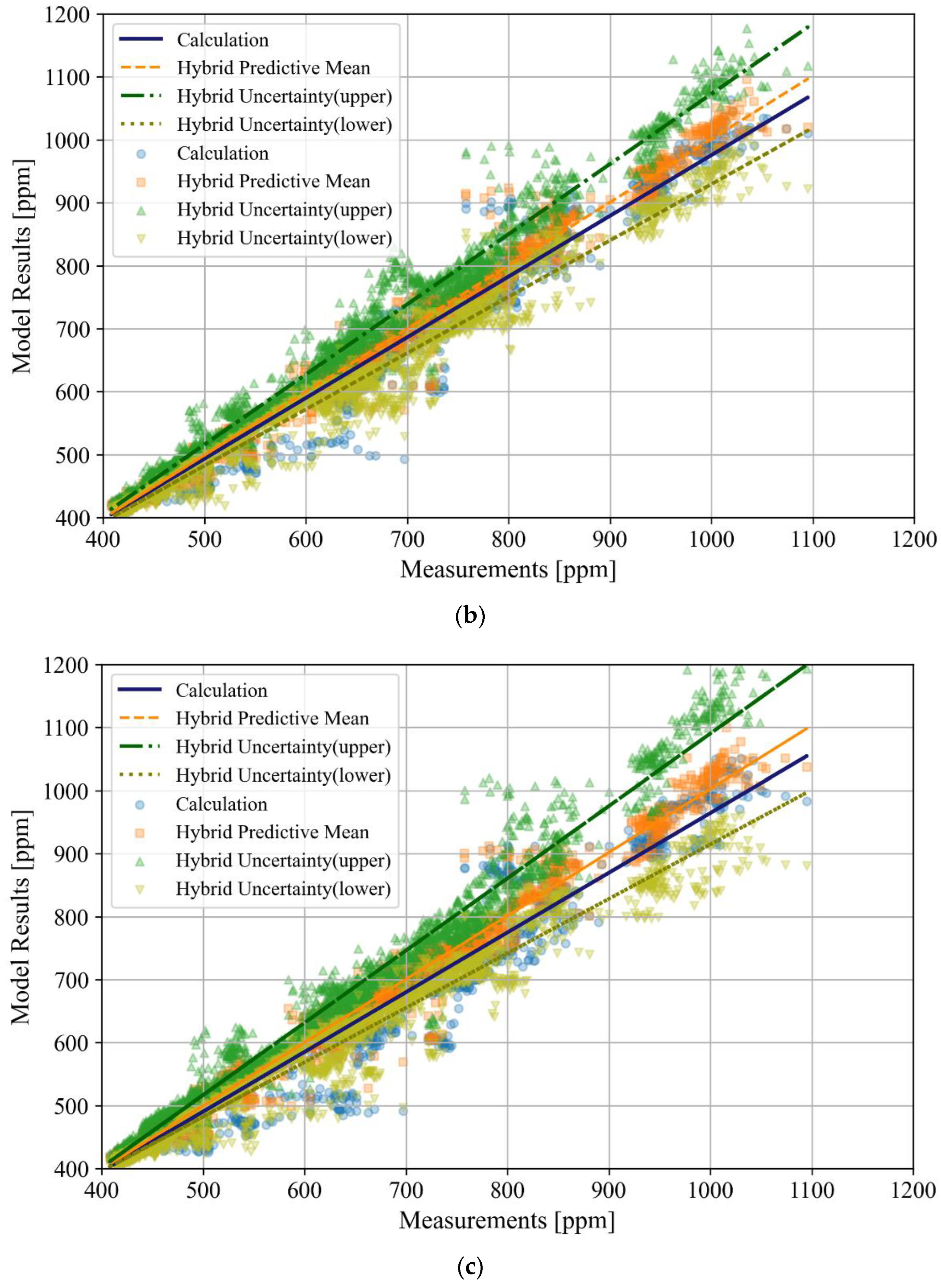
Figure 5 and Figure 6 display the scatter plots of the relationship between the measurement and forecasting results obtained using the hybrid model and mass balance equation for the LR and BR1 zones. In particular, the results obtained using the hybrid model can be represented as the predictive mean and upper and lower boundaries of the total uncertainty, which includes the aleatoric and epistemic uncertainties. In the scatter plots, the relationships between the measurements and results obtained from each model are represented by a line plotted using first-order linear regression.
The relationship between the measurement and forecasting results obtained from the mass balance equation shows that the variance gradually increases as the prediction horizon increases and the slope of the first-order linear regression line gradually decreases to less than 1 in the case of the LR zone.
The relationships between the predictive mean of the hybrid model and measurements for both the zones are linear, with a slope of almost one regardless of the change in the prediction horizon. This is in contrast with the relationship between the measurements and the results obtained using the mass balance equation. However, as the prediction horizon increases, the variance in the relationship between the predictive mean of the hybrid model and measurement increases. In addition, the slope of the first-order linear regression line for the upper boundary of the total uncertainty in the forecast of the hybrid model gradually increases and that of the lower boundary gradually decreases. More specifically, increasing the predictive uncertainty of the hybrid model based on the prediction horizon can be investigated using the hybrid model.
5. Conclusions
The indoor CO2 concentration can affect the health of occupants and is used as a metric of ventilation in buildings. To implement the MPC of a residential HRV, a hybrid model that combines the mass balance equation as the white-box model and a BNN as the black-box model was developed. In particular, the aggregated unknown ventilation rate term was added to the mass balance equation in the hybrid model to account for infiltration and interzonal airflow. The BNN in the hybrid model estimated the aggregated unknown ventilation rate during the learning process and transferred the estimation to the mass balance equation.
In this study, the measurement data containing the indoor CO2 concentration according to the varying ventilation rate of an HRV and the number of occupants were recorded in the LR and BR1 of a 59 m2 apartment unit. Two hybrid models were subsequently used to forecast the indoor CO2 concentration in LR and BR1 over the prediction horizon. To determine the appropriate prediction horizon for the MPC, the prediction horizons of 5, 10, and 15 min were tested on the hybrid model. Additionally, the forecasting performance of the hybrid model was compared with that of the stand-alone traditional mass balance equation for a single zone.
The results revealed that the forecasting accuracy of the hybrid models decreased as the prediction horizon was increased from 5 min to 15 min; however, the hybrid model exhibited better performance than that of the traditional mass balance equation in terms of three indicators namely, MBE, CVRMSE, and R2. Based on the longest prediction horizon of 15 min, the forecasting performances of the hybrid model for the indoor CO2 concentration in LR and BR1 were as follows: the MBE values were −0.01% and −1.28%, respectively, CVRMSE values were 3.24% and 7.21%, respectively, and R2 values were 0.99 and 0.955, respectively. In contrast, the forecasting performance of the mass balance equation for LR and BR1 were as follows: MBE values were −2.42% and 0.45%, respectively, CVRMSE values were 5.76% and 12.84%, respectively, and R2 values were 0.95 and 0.85, respectively.
In addition, the results of the hybrid model indicated that predictive uncertainty increased as the prediction horizon increased. When the prediction horizons were 5, 10, and 15 min, the total predictive uncertainties, which are a combination of the aleatoric and epistemic uncertainties of the hybrid model related to LR were 17.66 (=15.32 + 2.34), 26.42 (=22.78 + 3.64), and 29.68 (=24.38 + 5.3) ppm, respectively, and those related to BR1 were 20.89 (=16.26 + 4.63), 35.03 (=28.11 + 6.92), and 44.24 (=33.03 + 11.21) ppm, respectively. Therefore, the predictive uncertainty of the hybrid model is expected to be applied toward the implementation of a robust MPC for an HRV.
Since the number of occupants in a residential building can be counted, the number of occupants in LR and BR1 was recorded manually using advanced smart metering devices, and the standard CO2 generation rate per person was applied according to the gender of the occupants. In this study, an aggregated unknown term for the ventilation rate was applied to the hybrid model; however, considering that the CO2 generation rate may vary depending on the behavior of the occupants, multiple unknown terms will be investigated in future studies. In addition, parametric studies using the hybrid model will be conducted to verify reliability and explainability in terms of physically comprehensible predictions when changing the parameters of HRV.
Author Contributions
K.U.A. developed the model; K.C. conducted the experiments and collected datasets; K.U.A., D.-W.K., K.C., D.C., H.M.C. and C.-U.C. described the results presented in this paper. All authors have read and agreed to the published version of the manuscript.
Funding
This work was supported by the Land Transport Technology Promotion Project funded by the Ministry of Land, Infrastructure and Transport of Korean government [grant number 22CTAP-C163641-02].
Data Availability Statement
The data supporting the results reported in this study will be available upon request from the corresponding author.
Conflicts of Interest
The authors declare no conflict of interest.
Nomenclature
| Symbol | Title |
| BNN | Bayesian neural network |
| BR | Bedroom |
| Indoor CO2 concentration, mg/m3 | |
| Indoor CO2 concentration in living room, mg/m3 | |
| Outdoor CO2 concentration, mg/m3 | |
| Indoor CO2 concentration in bedroom#1, mg/m3 | |
| Bayesian neural network model (Section 3.2) | |
| Mass balance equation model (Section 3.1) | |
| CO2 generation rate per person, mg/s | |
| CO2 generation rate per person in living room, mg/s | |
| CO2 generation rate per person in bedroom#1, mg/s | |
| Prediction horizon | |
| HRV | Heat recovery ventilator |
| LR | Living room |
| Ventilation rate, m3/s | |
| Ventilation rate of HRV in living room, m3/s | |
| Ventilation rate of HRV in bedroom#1, m3/s | |
| Unknown ventilation rate, m3/s | |
| Ventilation rate of HRV, m3/s | |
| Zone volume, m3 | |
| Living room volume, m3 | |
| Bedroom#1 volume m3 | |
References
- Kallio, J.; Tervonen, J.; Rasanen, P.; Makynen, R.; Koivusaari, J.; Peltola, J. Forecasting office indoor CO2 concentration using machine learning with a one-year dataset. Build. Environ. 2021, 187, 107409. [Google Scholar] [CrossRef]
- Korea.net. Available online: https://www.korea.net/NewsFocus/policies/view?articleId=205222 (accessed on 4 August 2022).
- Korea.kr. Available online: https://www.korea.kr/news/policyNewsView.do?newsId=148894861 (accessed on 4 August 2022).
- Taheri, S.; Razban, A. Learning-based CO2 concentration prediction: Application to indoor air quality control using demand-controlled ventilation. Build. Environ. 2021, 205, 108164. [Google Scholar] [CrossRef]
- Walker, S.S.W.; Lombardi, W.; Lesecq, S.; Roshany-Yamchi, S. Application of distributed model predictive approaches to temperature and CO2 concentration control in buildings. IFAC-PapersOnLine 2017, 50, 2589–2594. [Google Scholar] [CrossRef]
- Erdmann, C.; Steiner, K.; Apte, M. Indoor Carbon Dioxide Concentrations and Sick Building Syndrome Symptoms in the Base Study Revisited: Analyses of the 100 Building Dataset. Lawrence Berkeley National Laboratory. Available online: https://escholarship.org/uc/item/1mf005ws (accessed on 4 August 2022).
- ASHRAE. ASHRAE Standard 62-Ventilation for Acceptable Indoor Air Quality; American Society of Heating, Refrigerating, and Air-Conditioning Engineers (ASHRAE): Atlanta, GA, USA, 1981. [Google Scholar]
- Lu, X.; Pang, Z.; Fu, Y.; O’Neill, Z. The nexus of the indoor CO2 concentration and ventilation demands underlying CO2-based demand-controlled ventilation in commercial buildings: A critical review. Build. Environ. 2002, 218, 109116. [Google Scholar] [CrossRef]
- World Health Organization. Air Quality Guidelines for Europe, 2nd ed.; European Series, No. 91; World Health Organization Regional Office for Europe: Copenhagen, Denmark, 2000; ISBN 9289013583. [Google Scholar]
- BS EN 13779; BS EN 13779-Ventilation for Non-Residential Buildings-Performance Requirements for Ventilation and Room-Conditioning Systems. British Standards Institution (BSI): London, UK, 2007.
- BS EN 15251; BS EN 15251-Indoor Environmental Input Parameters for Design and Assessment of Energy Performance of Buildings-Addressing Indoor Air Quality, Thermal Environment, Lighting and Acoustics. British Standards Institution (BSI): London, UK, 2007.
- Yang, R.; Wang, L. Development of multi-agent system for building energy and comfort management based on occupant behaviors. Energy Build. 2013, 56, 1–7. [Google Scholar] [CrossRef]
- Fisk, W.J. The ventilation problem in schools: Literature review. Indoor Air 2017, 27, 1039–1051. [Google Scholar] [CrossRef]
- Yao, Y.; Shekhar, D.K. State of the art review on model predictive control (MPC) in Heating Ventilation and Air-conditioning (HVAC) field. Build. Environ. 2021, 200, 107952. [Google Scholar] [CrossRef]
- Belic, F.; Hocenski, Z.; Sliskovic, D. HVAC control methods-a review. In Proceedings of the IEEE 19th International Conference on System Theory, Control and Computing (ICSTCC), Cheile Gradistei, Romania, 9 November 2015. [Google Scholar] [CrossRef]
- Afram, A.; Janabi-Sharifi, F. Theory and applications of HVAC control systems–A review of model predictive control (MPC). Build. Environ. 2014, 72, 343–355. [Google Scholar] [CrossRef]
- Privara, S.; Široký, J.; Ferkl, L.; Cigler, J. Model predictive control of a building heating system: The first experience. Energy Build. 2011, 43, 564–572. [Google Scholar] [CrossRef]
- Moroşan, P.D.; Bourdais, R.; Dumur, D.; Buisson, J. Building temperature regulation using a distributed model predictive control. Energy Build. 2010, 42, 1445–1452. [Google Scholar] [CrossRef]
- Yuan, S.; Perez, R. Multiple-zone ventilation and temperature control of a single-duct VAV system using model predictive strategy. Energy Build. 2006, 38, 1248–1261. [Google Scholar] [CrossRef]
- Thieblemont, H.; Haghighat, F.; Ooka, R.; Moreau, A. Predictive control strategies based on weather forecast in buildings with energy storage system: A review of the state-of-the art. Energy Build. 2017, 153, 485–500. [Google Scholar] [CrossRef]
- Ahn, K.U.; Park, C.S.; Kim, K.J.; Kim, D.W.; Chae, C.U. Hybrid model using Bayesian neural network for variable refrigerant flow system. J. Build. Perform. Simul. 2022, 15, 1–20. [Google Scholar] [CrossRef]
- Kendall, A.; Gal, Y. What uncertainties do we need in Bayesian deep learning for computer vision? arXiv 2017, arXiv:1703.04977. [Google Scholar] [CrossRef]
- Nannapaneni, S.; Mahadevan, S. Reliability analysis under epistemic uncertainty. Reliab. Eng. Syst. Saf. 2016, 155, 9–20. [Google Scholar] [CrossRef]
- Cho, K.; Cho, D.; Kim, T. Effect of bypass control and room control modes on fan energy savings in a heat recovery ventilation system. Energies 2020, 13, 1815. [Google Scholar] [CrossRef]
- Lawrence, T.M.; Braun, J.E. Evaluation of simplified models for predicting CO2 concentrations in small commercial buildings. Build. Environ. 2006, 41, 184–194. [Google Scholar] [CrossRef]
- Federspiel, C.C. Estimating the inputs of gas transport processes in buildings. IEEE Trans. Control Syst. Technol. 1997, 5, 480–489. [Google Scholar] [CrossRef]
- Federspiel, C.C. Conditions for the input-output relation of perfect-mixing processes to be first order with application to building ventilation systems. J. Dyn. Syst. Meas. Control 1998, 120, 170–176. [Google Scholar] [CrossRef]
- Ryu, S.; Kwon, Y.; Kim, W.Y. Uncertainty quantification of molecular property prediction with Bayesian neural networks. arXiv 2019, arXiv:1903.08375. [Google Scholar] [CrossRef]
- Der Kiureghian, A.; Ditlevsen, O. Aleatory or epistemic? Does it matter? Struct. Saf. 2009, 31, 105–112. [Google Scholar] [CrossRef]
- Gal, Y. Uncertainty in Deep Learning. Ph.D. Thesis, University of Cambridge, Cambridge, UK, 2016. [Google Scholar]
- Li, X.; Wen, J. Review of building energy modeling for control and operation. Renew. Sustain. Energy Rev. 2014, 37, 517–537. [Google Scholar] [CrossRef]
- Zhao, H.X.; Magoulès, F. A review on the prediction of building energy consumption. Renew. Sustain. Energy Rev. 2012, 16, 3586–3592. [Google Scholar] [CrossRef]
- Fumo, N. A review on the basics of building energy estimation. Renew. Sustain. Energy Rev. 2014, 31, 53–60. [Google Scholar] [CrossRef]
- Afram, A.; Janabi-Sharifi, F. Gray-box modeling and validation of residential HVAC system for control system design. Appl. Energy 2015, 137, 134–150. [Google Scholar] [CrossRef]
- Afram, A.; Janabi-Sharifi, F. Black-box modeling of residential HVAC system and comparison of gray-box and black-box modeling methods. Energy Build. 2015, 94, 121–149. [Google Scholar] [CrossRef]
- Coakley, D.; Raftery, P.; Keane, M. A review of methods to match building energy simulation models to measured data. Renew. Sustain. Energy Rev. 2014, 37, 123–141. [Google Scholar] [CrossRef]
- Pantazaras, A.; Lee, S.E.; Santamouris, M.; Yang, J. Predicting the CO2 levels in buildings using deterministic and identified models. Energy Build. 2016, 127, 774–785. [Google Scholar] [CrossRef]
- ASHRAE Standard 62.1; Ventilation for Acceptable Indoor Air Quality. ASHRAE Inc.: Atlanta, GA, USA, 2019.
- Korean Standard. KS F 2603; In Standard Test Method for Measuring Indoor Ventilation Rate (Carbon Dioxide Method). Korean Standard: Seoul, Korea, 2016.
Figure 1.
Target space and system. (a) Floor plan and duct configuration of the HRV. (b) Diagram of the HRV system. (c) VAV diffuser (left: Fully closed, middle: partially opened, right: Fully opened). (d) LR of the target space (left) and the FMS.
Figure 1.
Target space and system. (a) Floor plan and duct configuration of the HRV. (b) Diagram of the HRV system. (c) VAV diffuser (left: Fully closed, middle: partially opened, right: Fully opened). (d) LR of the target space (left) and the FMS.


Figure 2.
Concept and learning process of the hybrid model for forecasting indoor CO2 concentration; the inputs in the white box shown with a dotted line have identical values and are entered into and .
Figure 2.
Concept and learning process of the hybrid model for forecasting indoor CO2 concentration; the inputs in the white box shown with a dotted line have identical values and are entered into and .

Figure 3.
Time–series forecasting results obtained using the hybrid model and mass balance equation for the LR zone for the prediction horizons of (a) 5 min, (b) 10 min, and (c) 15 min for March 21 and (d) 5 min, (e) 10 min, and (f) 15 min for 22 March.
Figure 3.
Time–series forecasting results obtained using the hybrid model and mass balance equation for the LR zone for the prediction horizons of (a) 5 min, (b) 10 min, and (c) 15 min for March 21 and (d) 5 min, (e) 10 min, and (f) 15 min for 22 March.


Figure 4.
Time-series forecasting results obtained using the hybrid model and mass balance equation for the BR1 zone for the prediction horizons of (a) 5 min, (b) 10 min, and (c) 15 min for 21 March and (d) 5 min, (e) 10 min, and (f) 15 min for 22 March.
Figure 4.
Time-series forecasting results obtained using the hybrid model and mass balance equation for the BR1 zone for the prediction horizons of (a) 5 min, (b) 10 min, and (c) 15 min for 21 March and (d) 5 min, (e) 10 min, and (f) 15 min for 22 March.


Figure 5.
Scatter plot of the forecasting results obtained using the hybrid model and mass balance equation for the LR zone for the prediction horizons of (a) 5 min, (b) 10 min, and (c) 15 min.
Figure 5.
Scatter plot of the forecasting results obtained using the hybrid model and mass balance equation for the LR zone for the prediction horizons of (a) 5 min, (b) 10 min, and (c) 15 min.


Figure 6.
Scatter plot of the forecasting results obtained using the hybrid model and mass balance equation for the BR1 zone for the prediction horizons of (a) 5 min, (b) 10 min, and (c) 15 min.
Figure 6.
Scatter plot of the forecasting results obtained using the hybrid model and mass balance equation for the BR1 zone for the prediction horizons of (a) 5 min, (b) 10 min, and (c) 15 min.


Table 1.
Experimental cases.
| Experimental Case Index | Living Room (LR) | Bedroom#1(BR1) | ||
|---|---|---|---|---|
| Number of Occupants | Ventilation Rate (ACH) | Number of Occupants | Ventilation Rate (ACH) | |
| #1 | 0 | 0 | 1 | 0 |
| #2 | 0 | 0 | 1 | 0.5 |
| #3 | 0 | 0 | 1 | 0.7 |
| #4 | 0 | 0 | 1 | 1 |
| #5 | 0 | 0 | 2 | 0 |
| #6 | 0 | 0 | 2 | 0.5 |
| #7 | 0 | 0 | 2 | 0.7 |
| #8 | 0 | 0 | 2 | 1 |
| #9 | 0 | 0.5 | 1 | 0.5 |
| #10 | 0 | 0.7 | 1 | 1 |
| #11 | 0 | 1 | 1 | 1 |
| #12 | 1 | 0 | 0 | 0 |
| #13 | 1 | 0.5 | 0 | 0 |
| #14 | 1 | 0.7 | 0 | 0 |
| #15 | 1 | 1 | 0 | 0 |
| #16 | 2 | 0 | 0 | 0 |
| #17 | 2 | 0.5 | 0 | 0 |
| #18 | 2 | 0.7 | 0 | 0 |
| #19 | 2 | 1 | 0 | 0 |
| #20 | 3 | 0 | 0 | 0 |
| #21 | 3 | 0.5 | 0 | 0 |
| #22 | 3 | 0.7 | 0 | 0 |
| #23 | 3 | 1 | 0 | 0 |
Table 2.
Parameter settings of the BNN in the hybrid model.
| Parameter | Value |
|---|---|
| Number of hidden layers | 3 |
| Number of neurons in each hidden layer | 100 |
| Activation function in each hidden layer | ReLu |
| Dropout rate | 0.1 |
| Number of MC samplings | 100 |
| Number of epochs | 1500 |
| Mini-batch size | 500 |
| Optimization algorithm | Adam optimizer |
| Learning rate | 0.0001 |
Table 3.
Forecasting accuracy and uncertainty results.
| Model | Indicator | Prediction Interval | Target Zone | |
|---|---|---|---|---|
| LR | BR1 | |||
| Hybrid model | MBE [%] | 5 min | 0.07 | 0.02 |
| 10 min | −0.10 | 0.23 | ||
| 15 min | −0.01 | −1.28 | ||
| CVRMSE [%] | 5 min | 2.07 | 3.24 | |
| 10 min | 2.74 | 5.38 | ||
| 15 min | 3.24 | 7.21 | ||
| R2 | 5 min | 0.99 | 0.99 | |
| 10 min | 0.99 | 0.97 | ||
| 15 min | 0.99 | 0.95 | ||
| Aleatoric uncertainty (average) [ppm] | 5 min | 15.32 | 16.26 | |
| 10 min | 22.78 | 28.11 | ||
| 15 min | 24.38 | 33.03 | ||
| Epistemic uncertainty (average) [ppm] | 5 min | 2.34 | 4.63 | |
| 10 min | 3.64 | 6.92 | ||
| 15 min | 5.30 | 11.21 | ||
| Mass balance equation | MBE [%] | 5 min | −0.85 | 0.17 |
| 10 min | −1.65 | 0.33 | ||
| 15 min | −2.42 | 0.45 | ||
| CVRMSE [%] | 5 min | 2.95 | 6.04 | |
| 10 min | 4.28 | 9.24 | ||
| 15 min | 5.76 | 12.84 | ||
| R2 | 5 min | 0.99 | 0.96 | |
| 10 min | 0.97 | 0.92 | ||
| 15 min | 0.95 | 0.85 | ||
Publisher’s Note: MDPI stays neutral with regard to jurisdictional claims in published maps and institutional affiliations. |
© 2022 by the authors. Licensee MDPI, Basel, Switzerland. This article is an open access article distributed under the terms and conditions of the Creative Commons Attribution (CC BY) license (https://creativecommons.org/licenses/by/4.0/).
Share and Cite
MDPI and ACS Style
Ahn, K.U.; Kim, D.-W.; Cho, K.; Cho, D.; Cho, H.M.; Chae, C.-U. Hybrid Model for Forecasting Indoor CO2 Concentration. Buildings 2022, 12, 1540. https://0-doi-org.brum.beds.ac.uk/10.3390/buildings12101540
AMA Style
Ahn KU, Kim D-W, Cho K, Cho D, Cho HM, Chae C-U. Hybrid Model for Forecasting Indoor CO2 Concentration. Buildings. 2022; 12(10):1540. https://0-doi-org.brum.beds.ac.uk/10.3390/buildings12101540
Chicago/Turabian StyleAhn, Ki Uhn, Deuk-Woo Kim, Kyungjoo Cho, Dongwoo Cho, Hyun Mi Cho, and Chang-U Chae. 2022. "Hybrid Model for Forecasting Indoor CO2 Concentration" Buildings 12, no. 10: 1540. https://0-doi-org.brum.beds.ac.uk/10.3390/buildings12101540
Note that from the first issue of 2016, this journal uses article numbers instead of page numbers. See further details here.