The Impact of Climate Change on a University Campus’ Energy Use: Use of Machine Learning and Building Characteristics

Abstract

Global warming is expected to increase 1.5 °C between 2030 and 2052. This may lead to an increase in building energy consumption. With the changing climate, university campuses need to prepare to mitigate risks with building energy forecasting models. Although many scholars have developed buildings energy models (BEMs), only a few have focused on the interpretation of the meaning of BEM, including climate change and its impacts. Additionally, despite several review papers on BEMs, there is no comprehensive guideline indicating which variables are appropriate to use to explain building energy consumption. This study developed building energy prediction models by using statistical analysis: multivariate regression models, multiple linear regression (MLR) models, and relative importance analysis. The outputs are electricity (ELC) and steam (STM) consumption. The independent variables used as inputs are building characteristics, temporal variables, and meteorological variables. Results showed that categorizing the campus buildings by building type is critical, and the equipment power density is the most important factor for ELC consumption, while the heating degree is the most critical factor for STM consumption. The laboratory building type is the most STM-consumed building type, so it needs to be monitored closely. The prediction models give an insight into which building factors remain essential and applicable to campus building policy and campus action plans. Increasing STM is to raise awareness of the severity of climate change through future weather scenarios.

1. Introduction

Even though accelerating issues on climate change are arousing people’s awareness, many are still uninformed about how climate change affects building energy consumption. Building operations are responsible for 28% of total emissions, while embodied carbon, which is from building materials and construction, is responsible for an additional 11% annually [1]. This is nearly 40% of CO₂ emissions coming from the building and building construction sector, which is responsible for over one-third of global energy consumption [2]. Global warming—a product of climate change—is also expected to significantly increase building energy use for cooling. Climate change phenomena are not uniform across the globe, so energy consumption direction or protocol can differ by climate zone. Therefore, this study focuses on the energy use of a Philadelphia (PA)-based university’s campus under climate zone 4A, comprised of a humid subtropical climate [3].

College and university campuses use an average of 18.9 kilowatt-hours (kWh) of electricity (ELC) and 17 cubic feet (ft²) of natural gas per square foot annually [4]. Universities have consumed a large portion of energy use and have updated their sustainability plan to reduce greenhouse gas emissions and energy consumption. Universities serve as pioneers for green societies and make immediate decisions and policies to address climate change, compared to other national-level organizations. Since university campuses include various building types, such as libraries, offices, laboratories, hospitals, and housing, these installations remain uniquely positioned to analyze the energy consumption of “mixed-use” group buildings. Essentially, a college or university campus serves as an independent district. Thus, typical university campuses can offer informative representations of urban energy consumption.

To minimize energy consumption, building energy consumption patterns need to be monitored and analyzed. By doing so, universities identify ways to effectively manage energy use and plan building renovation with an understanding about the relationship between building characteristics and energy consumption. In addition, energy consumption prediction can be beneficial for universities to forecast reliable energy budgets and identify opportunities of energy conservation [5].

This study investigates global climate change’s influence on building energy consumption, the building’s behavior, and other energy-related factors on campus. In this case study, ELC and steam (STM) were considered. ELC was provided by Penn Power, and the STM distribution system consisted of underground pipelines. Building characteristics, meteorological variables, and temporal variables were used to develop BEMs with a bottom-up approach for ELC and STM consumption. Among various bottom-up approaches, a multivariate regression and multiple linear regression (MLR) were chosen.

Thanks to rapid technology development, electronic appliance efficiency is improving, and construction materials are evolving for better insulation. In addition, smart homes and intelligent cities are becoming more popular, and the number of electronic devices people own is rising fast. To eliminate complex interventions, the impact of climate change on the energy consumption of existing buildings is analyzed purely by excluding technological advances. Furthermore, occupancy behavior was not considered in the focus on weather features and building characteristics. Consequently, operation features such as set point temperature, fan schedules, HVAC schedule (heating and cooling), lighting schedule, class schedule, building-operation hours, and building use schedule (occupancy schedule) were excluded.

2. Literature Review

To determine the method for this research, the statistical analysis used in BEMs were examined. Additionally, research on the BEMs of university campuses were analyzed to narrow the target. Then, the status of climate change and how global warming will affect building energy consumption were investigated. Finally, based on previous literature reviews, variable selections from other research allowed us to decide how to structure the data frame. Additionally, via literature reviews, this study intends to investigate factors that affect energy consumption the through interpretation of statistical models, with the following research questions (RQ):

RQ1. What are the appropriate building- and weather-related variables to be included in the predictive model?

RQ2. What is the relationship between input variables and energy consumption (output) by energy types considered by relative importance?

RQ3. How will each energy type change with the effects of global warming?

2.1. BEMs Focused on Statistical Analysis

Several review articles have summarized and defined Urban Building Energy Modeling (UBEM) [6,7]. The prevailing UBEM has two opposite modeling approaches: top-down or bottom-up. The top-down approach works at an aggregated level, typically aimed at fitting historical timelines based on national energy consumption while the bottom-up approach is built up from data as disaggregated components.

Since this study is focused on the bottom-up approach, this paper specifically discusses regression modeling approaches. Baker and Rylatt used clustering, simple regression, and MLR [8]. Kavousian et al. used stepwise selection to choose predictors in a MLR model because all input variables are numeric, not categorical [9]. Hsu used a Bayesian multilevel regression model to analyze the value of different measurements for predicting energy use and found that benchmarking data alone explains energy use as well as benchmarking and auditing data together [10]. Zeng et al. considered the multivariate regression model to be the best method in the case study with simplified inputs related to building energy [11]. Walter and Sohn also developed a multivariate regression model to predict Energy Unit Intensity (EUI) by using numerical predictors and categorical indicator variables [12]. For example, numerical predictors were operating hours, occupant density, etc., and categorical indicator variables were climate zone, heating system type, etc. This model measured the contribution of building characteristics and systems-to-energy use based on the cross-validation (CV) approach.

Most previous research in BEMs has failed to interpret the BEM, used insufficient samples, or missed some important variables that are equipment power density (EPD) or meteorological variables. Most research has focused on maximizing performance accuracy of machine learning (ML) models and finding the best model by comparing different ML techniques. This research has shown the improvement of the ML models’ accuracy. According to Kikumoto et al., as a result of increasing temperature, energy simulation showed a 15% increase in the heat load of two residential buildings [13]. A small sample size for application made it difficult to generalize future energy consumption. However, protocol or interpretations of the final ML models were frequently missing, so this study aims to interpret the regression models with a larger sample size.

2.2. BEMs Focused on University Campuses

Owing to the trend of growing energy consumption, Hong et al. investigated the energy waste in universities and suggested optimization options of campus buildings in South Korea [14]. The amount of ELC had risen about 19.7% over three years because the equipment used for heat had increased. Hong et al. also found that higher monthly average temperatures led to more A/C use on campus [15]. They developed several energy saving scenarios to suggest possible solutions. Chung and Rhee observed that equipment loads and occupancy schedules of university buildings for education and research are difficult to control [16]. However, they found that universities have a high potential to reduce energy losses caused by unnecessary energy consumption, low thermal performance, and airtightness. Because of the many random users rather than the operators themselves in the university buildings, retrofitting the existing buildings into low-energy buildings is crucial [14].

Guan et al. analyzed the ELC, heating, and water usage of campus buildings in Norway, which has a similar climate with climate zone category 5A [17]. They said that UBEM plays a critical role in learning about the efficient energy planning of future urban energy systems and smart systems. Several Chinese universities and colleges have initiated sustainable education and developed incentive policies to encourage students and faculty members to save energy [15]. Universities in the U.S. have taken actions on energy policies and movement for green campus development.

2.3. Climate Change

Recently, more studies have aimed at the future impact on energy consumption owing to climate change. Examples include energy use over long-term climate change for use in life cycle assessment applications with nine typical Florida residential houses [18]. Additionally, Fathi et al. and Fathi and Srinivasan expanded the sample size and targeted a university campus instead of residential buildings, wherein Principal Component Analysis (PCA) and Autoregressive Integrated Moving Average (ARIMA) techniques were selected for energy prediction with climate change [19,20]. Another example is that Godoy-Shimizu et al. estimated urban-scale energy consumption using physics-based models for future weather [21].

Fumo and Rafe Biswas (2015) predicted total ELC using only outdoor dry-bulb temperature and added the global horizontal radiation to produce MLR models without considering building characteristics [22]. Higher resolution for the time interval, which was hourly data, leads to models with a lower quality than regression models using daily data. All three regression models (simple linear, simple quadratic, and MLR) with daily resolution had better R-square values but lower accuracies based on root mean square error (RMSE) than with hourly resolution.

Mohammadiziazi and Bilec used RF to analyze office buildings’ EUI due to climate change [23]. They found that energy consumption will increase between 8.9% and 63.1% compared to the 2012 baseline for different geographic regions between 2030 and 2080. Campagna and Fiorito found that 65% of studies on climate change impacts on building energy consumption focused on climate zone C [24]. Therefore, studying climate zone A in this study can contribute to mitigating biased sample selection.

3. Methods

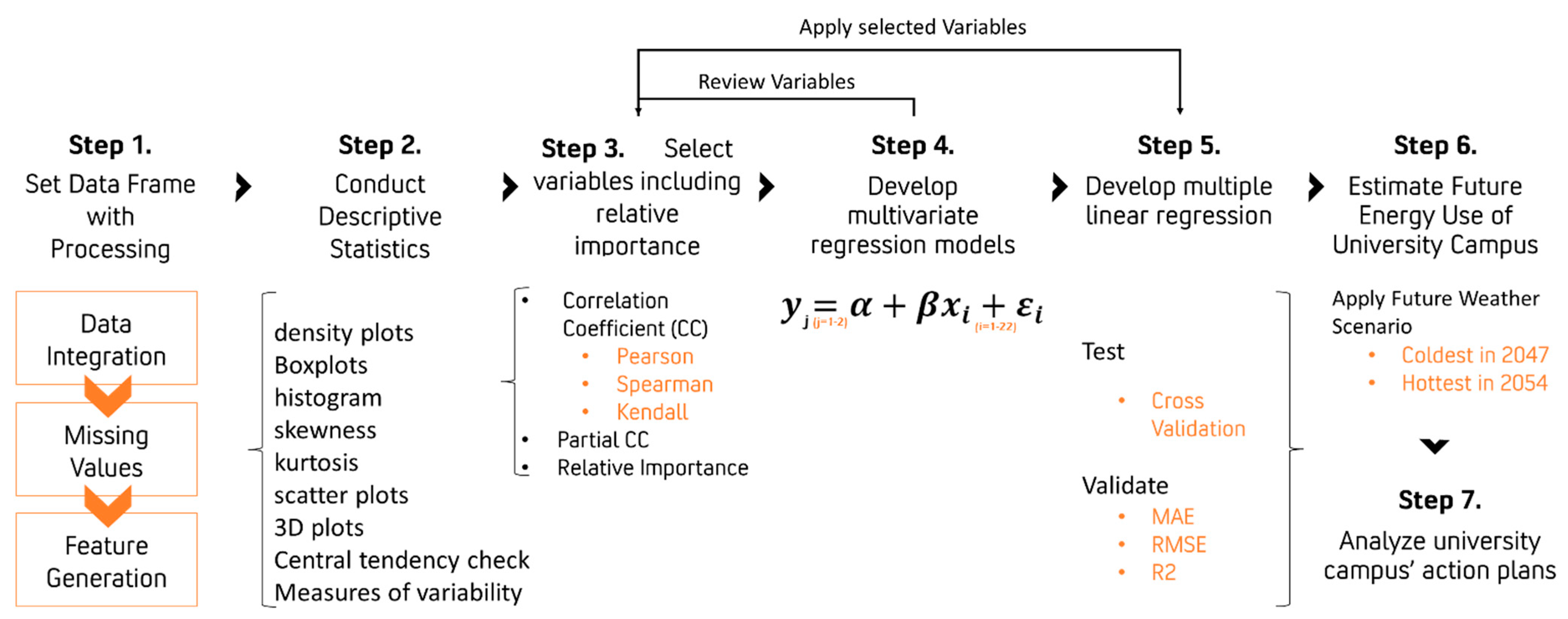
In this study, the hourly energy consumption data were obtained, which consist of ELC and STM. To answer the research questions, the BEMs’ development process follows six-steps, namely: (1) set data frame with processing, (2) conduct descriptive statistical analysis, (3) select variables including relative importance analysis, (4) develop multivariate regression models, (5) develop multiple linear regression (MLR) models, (6) estimate energy use of a university campus with future weather data, and (7) analyze university campus’ action plans (Figure 1).

Step 1 is setting data frame with processing. Four separate datasets (energy consumption variables, building variables, meteorological variables, and temporal variables) were merged to form one complete dataset. After collecting and cleaning all the data, the merged data was divided into a training and a testing dataset. The training dataset is from 1 July 2015 to 30 June 2016. For validation, a 10-fold cross-validation was conducted. The testing dataset is from 1 July 2016 to 14 August 2016.

Step 2 is conducting a descriptive statistical analysis. To observe the distribution, density plots, boxplots, histogram, skewness, and kurtosis were used. To understand the data and to detect outliers, scatter plots, three-dimensional (3D) plots, relative importance, correlation coefficient (CC), partial CC, and CC matrix plots are used. Additionally, central tendency (mean, mode, and median), measures of variability (range and interquartile range), variance, and standard deviation were measured.

Step 3 is selecting variables, including importance analysis. The multivariate regression method was used to determine independent variables because all buildings share the same independent variables. Based on other literatures and experts in machine learnings and statistics, different variables for multivariate regression models were used and compared to each other based on R² and RMSE. Four sets of multivariate regression models were developed, consisting of two linear regression models for ELC and STM. For reliable predictions, a large amount of historical data is required. Thus, the hourly data of 18 buildings with 22 input (independent) variables and 2 (dependent) variables were each observed and used to meet the requirement to develop the multivariate regression models.

The variables were analyzed based on CC, partial CC, and relative importance. To check correlations between variables, three CC measuring methods were used: (1) Pearson CC with the linear dependence between two numeric variables, (2) Spearman for polynomial relationship, and (3) Kendall between categorical input variables and numeric output variables. Kendall’s tau and Spearman’s rho were used to estimate a rank-based measure of association. To examine the categorical variables, we referred to relative importance as well. For relative importance, rank bootstrap confidence intervals were obtained by using the percentile method. Bootstraps were replicated 100 times in order to calculate confidence intervals. Metrics for relative importance are normalized to sum to 100%. This was used for all numeric variables and meteorological variables alone to examine the influence of variables on energy consumption. Lastly, partial CCs were measured to select meaningful variables.

Step 4 is developing multivariate regression models. From MLR development, variables were selected to finalize the multivariate regression model. As shown in Equation (1), independent numeric variables were standardized with a mean (μ) of 0 and standard deviation (σ) of 1 (unit variance):

X′ = (X − μ)/σ

(1)

Step 5 is developing MLR Models BEMs. As a feature selection method, stepwise selection methods were used. The performance was measured through Mean Absolute Error (MAE), RMSE, and adjusted R square (R²). MAE is a key performance indicator (KPI) for measuring forecast accuracy. These measures are used to check the regression model’s accuracy to validate and test and can be calculated using Equations (2)–(4):

$$\mathrm{MAE}=\frac{1}{n}{{\displaystyle \sum }}_{i=1}^n|y_{predict,i}-y_{data,i}|$$

(2)

$$\mathrm{RMSE}=\sqrt{\frac{{{\displaystyle \sum }}_{i=1}^n{\left(y_{predict,i}-y_{data,i}\right)}^2}{n}}$$

(3)

$${\mathrm{R}}^2=1-\frac{{{\displaystyle \sum }}_{i=1}^n{\left(y_{predict,i}-y_{data,i}\right)}^2}{{{\displaystyle \sum }}_{i=1}^n{\left(y_{data,i}-y_{data,i}\right)}^2}$$

(4)

According to Hoff and Perez, MAE is commonly accepted as a measure of dispersion because of its lesser sensitivity to distant outliers and lesser subjection to interpretation when expressed in relative (percentage) terms [25]. A 10-fold CV was used to validate BEMs and, to test the models, regression models’ accuracies were checked with a validation dataset. Based on MLR models, significant variables for each energy consumption type are revealed.

The sixth step is to estimate the energy use of university campuses with future weather data. As the last step, to estimate the operational energy consumption under long-term climate change, the average values from the hottest scenario representing 2054 were used as inputs into the MLR models. Likewise, the average values of building characteristics were used to predict energy consumption in 2054. Lastly, Step 7 is to analyze university campus’ action plans to learn lessons explained in Section 5.6. Specifically, in my research, energy action plans of 18 universities were analyzed to show how a leading energy group deals with climate change.

4. Variable Selection

From Step 1 to Step 3, potential independent variables were scrutinized to build BEMs to explain energy consumptions. This section demonstrates details about the variable selection process, which includes a literature review and the analysis of results.

It should be noted that Kikumoto et al. did not include the building characteristics in predicting heat loads [13]. Whereas Im et al. concentrated on interpreting the regression models to explain the relationships among building characteristics, energy consumption, and weather [26,27], Im et al. (2019) developed polynomial regression models on chilled water (CHW) and ELC consumption of campus buildings by comparing BEMs with hourly and daily data [24]. Additionally, Im et al. (2020) attempted to predict CHW with lasso regression models using future weather data [25]. However, both studies did not use solar radiation data, which is considered a significant factor in BEM [28]. In conclusion, this study focused on variable selection and the interpretation of BEMs with larger sample sizes, as well as additional building characteristics and weather data, including solar radiation. Considering ELC and STM allows us to grasp campus energy consumption comprehensively.

Out of 194 buildings, 48 buildings had one year of two energy consumption information: ELC and STM. Out of 48 buildings, 18 buildings’ data were used after excluding buildings missing building characteristics data to develop building energy modeling (BEM) by adopting multivariate regression models with a 14.5-month period. Developing multivariate regression models is to achieve a comprehensive understanding of energy use depending on the energy type by comparing the variables’ impact. The sample size could be larger when final regression models were developed separately, like 43 buildings for ELC and 32 buildings for STM (

Table 1. Building number by energy types and building types.

Building Type	ELC	STM
Education Laboratory Lodge	7	4
	8	7
	6	7
Office Public Assembly	10	6
	8	6
Food	3	1
Health	1	1
Sub-total number of buildings	43	32
Total number of buildings	39	30

). From these separate data frames, building types with less than three buildings were eliminated because of the small size in the number of buildings. As a result, all food and health-related buildings were eliminated. Eventually, 39 buildings for ELC and 30 buildings for STM were secured for multiple regression model analysis with the same time frame.

4.1. Energy Consumption Variables

Energy consumption variables were comprised of electricity consumption (ELC, kilo-British Thermal Unit (kBTU)/Gross Square Feet (GSF)) and steam consumption (STM, kBTU/GSF). Gross square feet (GSF) is highly related to several variables that have a value per unit square feet, such as U-values, EPD, and LPD. Therefore, GSF was included as a denominator of the dependent variable by dividing energy consumption data in kBTU with GSF. Equipment, lighting, and plug loads are three main categories contributing to the energy consumptions in the buildings. Equipment, such as heating, ventilation, and air conditioning (HVAC) systems and water heaters, is the other main internal load, which contributes to STM in this case study. Lighting and plug loads contribute to ELC. Plug loads are growing as electronics become more pervasive with the ever-accelerating progress of technology, even in construction, which used to be known as a conservative field.

4.2. Building Variables

Building variables comprised of building thermo-physical properties and other power densities. Building variables included the U-value of Wall (U-Wall, Btu/h °F.ft²), U-value of Windows (U-Windows, Btu/h °F.ft²), U-value of Roof (U-Roof, Btu/h °F.ft²), Window-Wall Ratio (WWR), building height (feet), construction year (year), Building Age (year), Renovation Age (year), equipment power density (EPD, W/ft²), and Lighting Power Density (LPD, W/ft²).

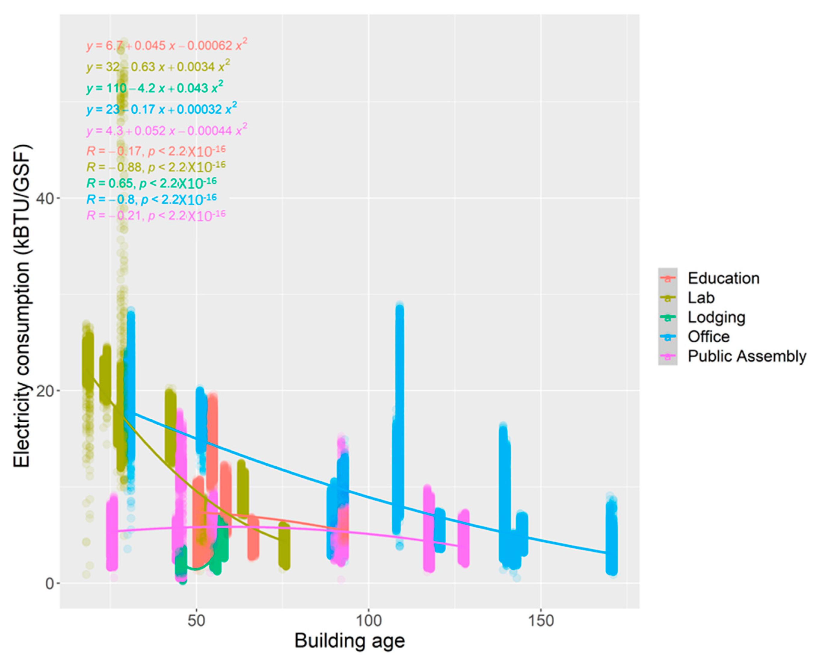
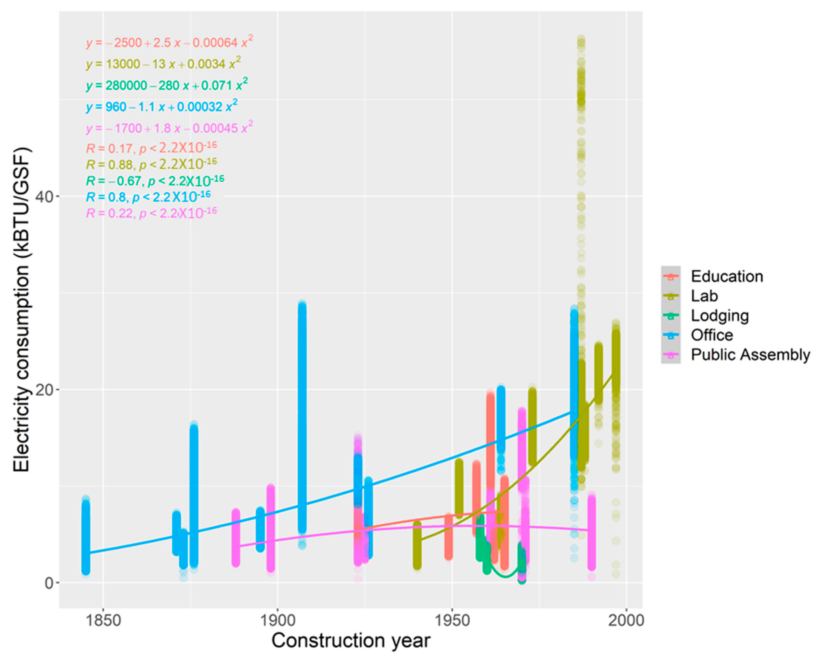
Based on the regression and the plot, the beta coefficient (β: slope of the regression models) shows that ELC consumption and Building Age are statistically, negatively related (Figure 2). The initial plot with Building Age could lead to the misinterpretation of energy consumption, which indicates that buildings consume less energy as time goes by, regardless of the deterioration of the building. Thus, it is important to use construction year instead of building age. As shown in Figure 3, ELC consumption is higher in newer buildings than in older buildings. This may be because buildings are evolving with advanced technology and more outlets. Newer buildings have more opportunity (more outlets or electronic appliances) of energy use compared to older buildings.

Gao et al. selected four variables (wall area, building height, building orientation, and glazing area) through the feature reduction process to improve the performance of models out of eight independent variables (relative compactness, surface area, wall area, roof area, building height, orientation, glazing area, and glazing area distribution of a residential building) [29]. Compared to the study by Gao et al., in this study, window wall ratios (WWR) were used, which is a combination of wall area and glazing. Building orientation was not used.

Godoy-Shimizu (2018) mentioned that several studies considered building height to estimate the building energy performance [18]. Additionally, a survey of the literature showed no previous studies used building height and the number of floors at the same time. Even though Capozzoli et al. considered both building height and the number of floors to predict heating energy consumption in schools, they a had too-low Pearson CC to include them in the MLR model [30]. Therefore, they excluded both variables in the MLR model because of the low CC.

Im et al. (2019) used the number of floors, the building height, and their interaction term in previous research and found that they are significant considering the p-value [21]. However, the number of floors was removed from the regression model due to high multicollinearity (Pearson CC: 0.9). The building height improved the regression models better than the number of floors. Using both building height and the number of floors might be worthy to research in commercial building because of its variety of space and height. Lastly, the year of building renovation was never used for building energy prediction. Furthermore, Construction Year was used to be the input of the BEM.

4.3. Meteorological Variables

Meteorological variables included solar radiation, outdoor air temperature, heating degree (HD), cooling degree (CD), relative humidity, pressure, and wind speed. The future meteorological data was obtained through the open source from the nonprofit energy weather research organization the Slipstream Group [25]. They developed the weather scenarios as a representative location for each ASHRAE climate zone with their proprietary algorithm. The mentioned algorithm uses raw climate data for future weather from the NARCCAP (North American Regional Climate Change Assessment Program). Future weather scenarios for Pennsylvania (PA) were unavailable; however, those scenarios for Baltimore, Maryland (MD) were available, which is in the same climate zone 4 and moist (A) category as PA. Predicted Maryland weather data has three future weather scenarios—coldest (2047), average, and hottest (2054). The hottest weather scenario of MD was chosen to consider the biggest impact on global warming.

The preliminary studies by Im et al. used two independent meteorological variables: (1) outdoor air temperature and (2) relative humidity, representing years 2015, 2016, and 2054 [26,27]. Common factors were selected among 15 historical meteorological variables and 11 future meteorological variables. There were four climate variables in common: temperature, humidity, pressure, and wind speed. Fathi and Srinivasan (2019) used temperature, solar radiation, and humidity as meteorological factors [20]. Daut et al. (2012) also revealed a strong linear relationship between solar radiation and surface temperature [26]. Therefore, solar radiation was added to the four climate variables as a final list in this study. HD and CD were generated from temperature with the setpoint standard 18.33 °C (65 °F). Because of the high multicollinearity, temperature and HD/CD cannot be used together.

4.4. Temporal Variables

Temporal variables included the number of the week throughout the year (week’s mumber), type of day (weekday, Saturday, or Sunday), numeric hour, categorical hour (0–23), hour type (working, evening, or night), business day type (business day or non-business day), and season type (spring, summer, fall, or winter).

According to Wang and Srinivasan, some researchers utilized occupancy indicators such as the time of day and day type [31]. For example, Dong et al. used the time of the day as a categorical variable to predict building energy consumption [28]. Dong et al. and Kotchen used the month of the year as a categorical variable [32,33]. Based on literature review and an expert’s opinion in Information Systems and Operations Management, in this study, temporal variables used as occupancy indicators are type of day, numeric hour, categorical hour, hour type, and business day type. These temporal variables allow for observation of the occupancy condition and pattern by remedying the missing occupancy information. Boiron et al. used the month, day of the week, and hour to develop a regression model [34]. This can be effective for observing behavior patterns at residential buildings, but it does not reflect change over time despite slight improvements in R² of campus data. Additionally, there is less of an opportunity to change human behavior in the campus setting than to change the technology and machinery being used by the buildings. Season type was used instead of the month of the year in this study to consider the campus’s characteristics. As a result, data were grouped into four seasons based on the academic calendar.

Both ELC and STM are consumed by occupants, so the presence of the users makes the difference in energy consumption. Therefore, holiday and non-holiday were separated as categorical variables. In addition, electricity consumption is for other uses rather than cooling and heating such as appliances, electronics, and lab equipment.

5. Results

5.1. Process of Variable Selection (Multivariate Regression Model Development)

Multivariate regression models were developed with 177,408 observations to estimate the ELC and STM consumption (

Table 2. Different Variables Sets Input in Multivariate regression models.

Input Variables	Data Type	Test 1	Test 2	Test 3	Test 4
X1U-Wall	Numeric	◉	◉	◉	◉
X2U-Window	Numeric	◉	◉	◉	◉
X3U-Roof	Numeric	◉	◉	◉	◉
X4WWR	Numeric	◉	◉	◉	◉
X5Bldg.Height	Numeric	◉	◉	◉	◉
X6-1Const.Year	Numeric				◉
X6-2Bldg.Age	Numeric	◉	◉	◉
X6-3Renov.	Numeric	◉	◉	◉	◉
X7Date	Numeric	◉
X8EPD	Numeric	◉	◉	◉	◉
X9LPD	Numeric	◉	◉	◉	◉
X10Solar	Numeric	◉	◉	◉	◉
X11-1Temp.	Numeric	◉	◉	◉
X11-2HD	Numeric				◉
X11-3CD	Numeric				◉
X12Humid.	Numeric	◉	◉	◉	◉
X13Pressure	Numeric	◉	◉	◉	◉
X14WindSpeed	Numeric	◉	◉	◉	◉
X15Weeknum	Numeric		◉	◉
X16Type of day	Nominal	◉	◉	◉
X17-0Numeric Hour	Numeric			◉
X17Categorical Hour 1–23	Ordinal		◉
X18Hour Type 1–2	Ordinal				◉
X19Business day Type	Nominal				◉
X20Bldg Type 1–4	Nominal				◉
X21Season Type 1–3	Ordinal				◉
X22: X2 × X4	Numeric				◉
X23: X6-1 × X6-3	Numeric				◉
X24: X1 × X4	Numeric				◉
Average RMSE		2.78	2.71	2.6	2.12
Average R2		0.66	0.66	0.68	0.81

). All numeric predictors were normalized to compare the β coefficient regardless of the unit of the variables. These models were developed with four sets of different variables. Variables in Test 1 consist of 15 numeric variables and one nominal variable. Variables in Test 2 consist of 15 numeric variables, a nominal variable, and one ordinal variable. Variables in Test 3 consist of 15 numeric variables and one nominal variable. Variables in Test 4 consist of 18 numeric variables including three interaction terms, two nominal variables, and two ordinal variables. R² and RMSE in Table 2 are averaged values of two models for ELC and STM. Detailed information with β coefficients is shown in Appendix A.

There was an overlap between time variables and weather information, which reflects seasonal changes. Meteorological variables’ change, construction year, and Renovation Age are reflected by time. Therefore, year, month of the year, and day were excluded for regression analysis. Adding Categorical Hour and Week’s Number to Test 2, instead of only the Date as in relative importance with bootstrap confidence interval were analyzed with a one-year train dataset.

Test 1 improved the ELC and STM models’ accuracy based on RMSE. Week’s number was used in Test 2 and Test 3 to observe the chronological order. Because of the continuous cyclical feature of the hour, the numeric hour was used in Test 3 and transformed with sine and cosine. Then, in both cases (ELC and STM), the models’ accuracy and R² improved. As a final step, new variables were added based on expert feedback in statistics, and some variables were eliminated. On top of three interaction terms (X22: X1_U-Window × X4_WWR, X23: X6-1_{Construction Year} × X6-3_Renov., X24: X1U-_Wall × X4 _WWR), four new variables are construction year instead of building age, hour type, building types, and business day type. Business day type was used to consider holidays instead of the type of day. The temperature was used initially in Test 1 through Test 3, but the R² and RMSE showed improvement in terms of the statistical model’s accuracy and explanation of energy consumption when HD and CD were considered instead of temperature. The last change in variables enhances all two models significantly. Inaccuracy of ELC MLR were increased based on higher RMSE, but R² was improved.

Based on the result of Test 2, among temporal variables, the hour variable was analyzed as a categorical variable. The MLR model for ELC, 6 am–10 pm, showed a significant p-value while 11 pm–5 am was insignificant, which was the nighttime, when people were asleep. For STM, the days of the week and 4 am–8 pm were significant. The rest of the hour variables were not. Descriptive data analysis is performed to capture the behavior of energy consumption over time. The hour variable is insignificant for STM, but a predictable pattern was observed in ELC (continuous increase from 3 am to 2 pm and continuous decrease during the rest of the time). Therefore, the hour variable was required by adopting sine and cosine as a periodical factor.

In conclusion, ELC usage had the longest hour timeframe that showed a meaningful difference with other times. STM was the next. According to the 2D plots, only ELC had an hourly consumption pattern as a cycle of the day, particularly owing to occupancy behavior rather than weather. Therefore, the hour variable for the ELC model, rather than STM, needed to be considered based on the findings in the multivariate regression model and descriptive analysis. Additionally, week number were insignificant for ELC. Thus, this study used multivariate analysis to compare the impact of variables for each type of energy consumption in order to grasp campus energy consumption comprehensively.

A lower U-value is better insulation for energy consumption. This applies to WWR because a high window rate compared to the wall can increase the chance of infiltration, leading to more cooling in the summer or heating in the winter season. Therefore, positive relationships are expected between the U-value of wall, the U-value of window, and the U-value of roof and energy consumption as well as between WWR and energy consumption. Final multivariate regression models were developed with 177,408 observations and 19 predictors with 3 interaction terms, consisting of 3 MLR models for ELC and STM (

Table 3. Building number by energy types and building types.

Building Type	ELC	STM
X1U-Wall X2U-Window X3U-Roof	0.084	−0.131
	−0.137	−0.001
	0.358 **	0.103
X4WWR X5Bldg.Height	−0.279 *	−0.086
	0.056	0.130
X6-1Const.Year	−0.267 *	−0.115
X6-3Renov.Age	−0.257 *	0.139
X8EPD	0.458 **	0.157
X9LPD	0.070	0.070
X10Solar	0.124	0.123
X11-2HD	0.008	0.392 *
X11-3CD	0.0315	−0.059
X12Humid.	−0.034	−0.033
X13pressure	−0.007	0.021
X14WindSpeed	0.042	0.045

Notes: Correlation is significant at different levels (2-tailed) as follows: ** 0.001 level and * 0.01 level.

).

5.2. Comparison of Multivariate Regression Model by Energy Type

Among building variables, there were three outstanding β coefficients in the multivariate regression model (

Table 4. Multivariate regression model (18 buildings) without standardization.

Building Type (Unit: kBtu/GSF)	ELC	STM
Intercept X1U-Wall X2U-Window	588.71	120.81
	53.48	35.20
	22.05	−12.53
X3U-Roof X4WWR	−10.53	−3.27
	160.66	24.36
X5Height	0.15	−0.01
X6-1Construction Year	−0.30	−0.07
X6-3Renov.	−15.33	−0.41
X8EPD	1.00	0.79
X9LPD	−3.71	2.80
X10Solar	−0.01	0.00
X11-2HD	−0.43	0.23
X11-3CD	1.29	−0.06
X12Humid	0.03	0.00
X13Pressure	−0.04	0.01
X14WindSpeed	−0.13	0.06
X15bldg Type_Lab	7.98	10.87
X15bldg Type_office	−2.83	−2.08
X15bldg Type_public	7.99	4.18
X18-1Hour Type_night hour	−0.51	−0.11
X18-2Hour Type_working hour	−1.52	0.39
X19Business Day Type_business day	−0.55	−0.04
X21-1Season Type_spring	−1.20	−0.17
X21-2Season Type_summer	1.77	−0.16
X21-3Season Type_winter	−0.31	0.04
X22: X2 × X4	−155.71	−98.53
X23: X6-1 × X6-3	−145.48	7.73
X24: X1 × X4	0.01	0.00
Adjusted R2 (%)	94.71	66.17

). ELC had a high β coefficient with EPD (1.58), compared with STM (1.24). STM had a positive β coefficient with a U-Window (0.61), opposite to ELC (−0.81). STM had a higher beta with building height (0.751), compared with meteorological ELC (0.349).

Among variables, solar radiation and wind speed were insignificant for ELC, considering the 0.05 level of p-values. Additionally, the week (Monday to Friday) was significant, but differentiating Saturday and Sunday was meaningless. Therefore, for ELC, categorizing the day of the week into business day or non-business day is better than the type of week. Both ELC and STM have negative β coefficients with temperature, which are −0.049 and −1.729, respectively.

5.3. Result of MLR

Cross-validation was conducted for the validation, and

Table 5. Multiple linear regression.

Building Type	ELC	STM
Intercept X1U-Wall X2U-Window	7.33	4.37
	1.39	−0.09
	−0.81	0.61
X3U-Roof X4WWR	1.31	0.99
	2.18	1.34
X5Height	0.31	0.52
X6-1Construction Year	3.33	2.37
X6-3Renov.Age	29.04	60.51
X8EPD	1.58	1.24
X9LPD	−0.51	-
X10Solar	−0.04	0.08
X11HD	0.03	1.55
X11CD	0.46	−0.20
X12Humid.	0.02	0.03
X13Pressure	−0.05	0.05
X14WindSpeed	−0.03	0.11
X18-1Hour Type_night	−0.17	−0.08
X18-2Hour Type_working	0.18	0.18
X19Bizday_business day	−0.24	−0.02
X20-1bldg Type_Office	1.78	0.90
X20-2bldg Type_Lab	1.07	−0.47
X20-3bldg Type_Lodge	−1.25	−0.15
X20-4bldg Type_Public	0.63	0.16
X21-1Season Type_Spring	−0.01	0.03
X21-2Season Type_Summer	−0.57	−0.02
X21-3Season Type_Winter	−0.70	−0.01
X22: X2 × X4	−1.17	−1.07
X23: X6-1 × X6-3	−29.54	−61.06
X24: X1 × X4	−2.20	−0.81
Adjusted R2 (%)	76.74	56.59

shows the MLR models’ results. The MLR model could explain 76.74% of the ELC consumption and 56.59% of STM based on R². The R² of ELC was the highest among the three energy consumption types for validation. Additionally, MAE, RMSE, and R² were measured to check the regression model’s accuracy to test as shown in

Table 6. BEMs’ accuracy test result of MLR.

	ELC	STM
Length X Mean Y Mean	39,072	29,568
	7.33	2.54
	7.33	2.54
MAE RMSE	0.00	0.01
	2.62	1.62
Adjusted R2 (%)	88.28	74.47

. ELC and STM had similar values in MAE (0.00 and 0.01) and RMSE (2.62 and 1.62). The R²s of model accuracy were ELC (88.28) and STM (74.47), respectively.

5.4. Relative Importance Analytics

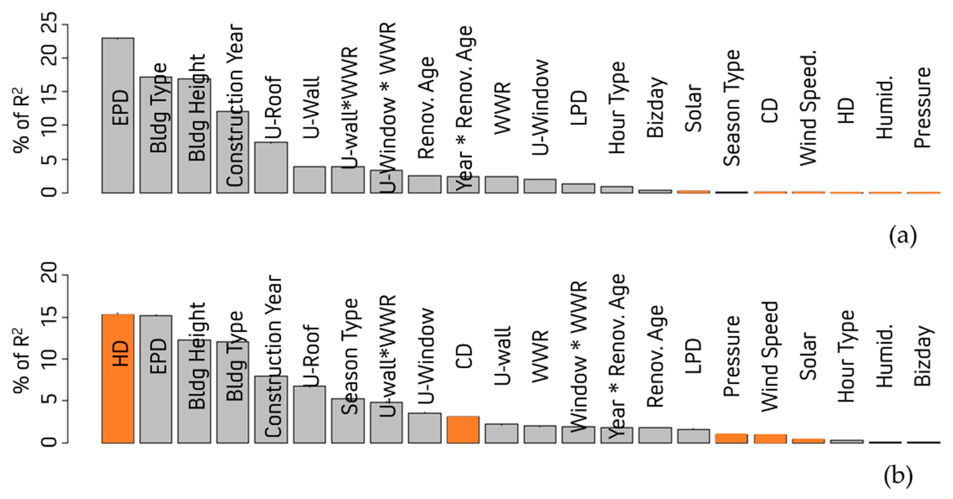
Relative importances with bootstrap confidence intervals (%) were analyzed with a one-year train dataset (177,408 observations), and metrics were normalized to sum to 100% (Figure 4).

Meteorological variables explained 0.06% (relative importance: 0.36%) for ELC and 4.36% (relative importance: 20.51%) for STM as revealed from R² of multivariate regression models. The relative contribution of solar radiation for ELC is 0.19% despite the low relative contribution rate as a most-related variable among weather variables. The relative contribution of temperature for ELC is 0.12%, which consists of CD: 0.11% and HD: 0.01%. The relationship between outdoor temperature and heating/cooling is obvious, but the relative importance analysis confirms the contribution of temperature to energy consumption. Based on relative importance analysis, HD is the most crucial predictor to predict STM. CD is the next crucial variable among meteorological variables, but other variables come prior to CD. When only weather variables were considered, relative contributions with 95% confidence intervals for HD are between 82.64% and 85.16% for STM. Relative contributions with 95% confidence intervals for CD are between 82.64% and 85.16% for STM. With other all variables, relative contributions for HD are 15.26% for STM. Relative contributions for CD are 3.07% for STM. Universities need to be aware of climate change because temperature-related variables are the top variable for STM. According to CD’s rank for STM, only HD was a significantly important variable for STM consumption, and a temperature below 65 °F did not affect the heating significantly.

Proportions of variance explained by the models were the same as adjusted R² of multivariate regression models. To answer RQ1, the top four variables that accounted for more than 50% of the relative importance were as follows: EPD, building type, building height, and construction year for ELC; HD, EPD, building height, and building type for STM. building height are common for both energy type. EPD, construction year and building type are common for ELC and STM. Therefore, universities should choose energy efficient EPD and decide on reasonable building height in the design phase to save ELC and STM consumption. Additionally, building energy should be analyzed by building type because the laboratory building type showed totally different patterns compared to other building types.

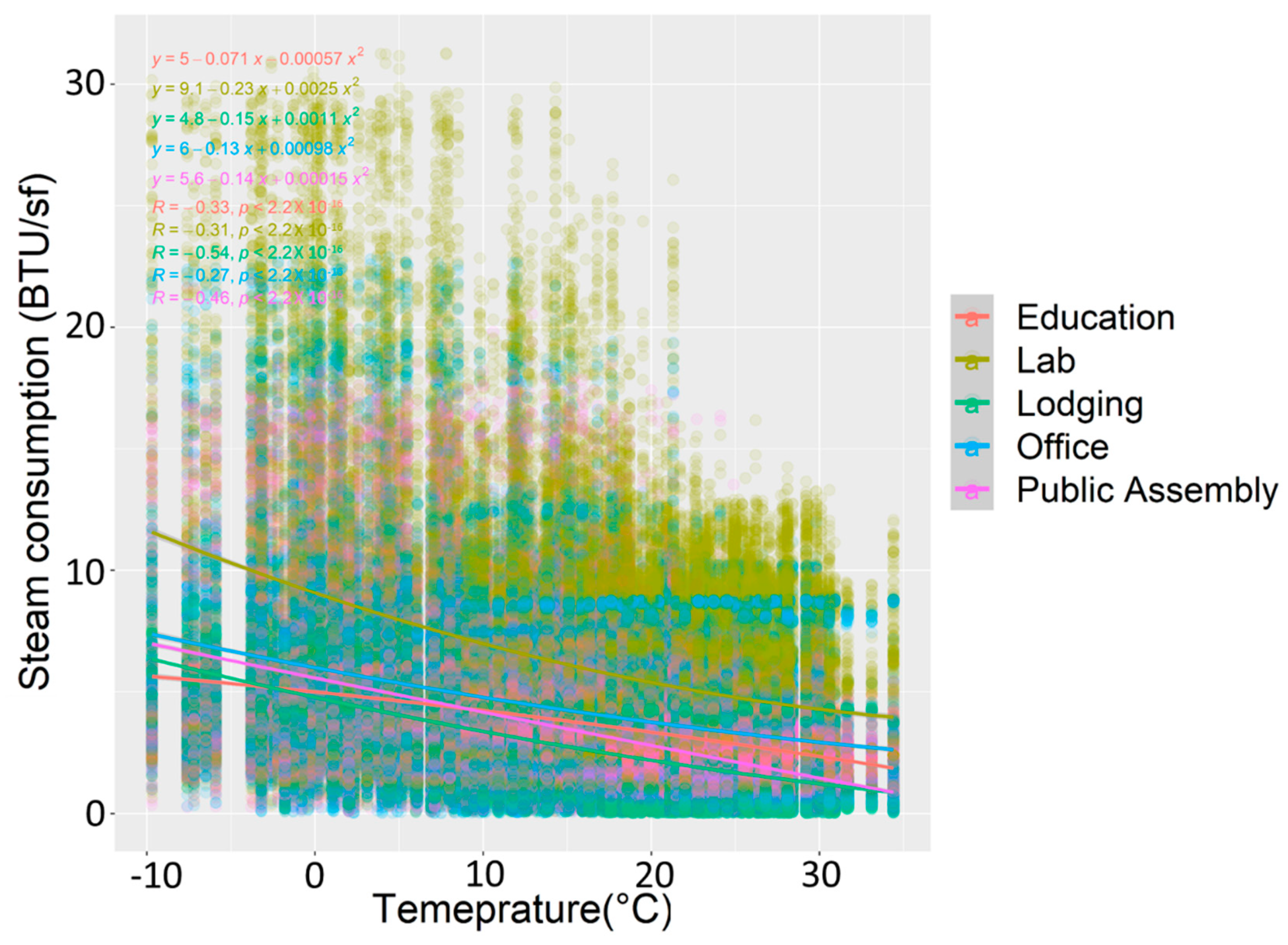
To be specific, energy consumption patterns by building type are analyzed as follows: through descriptive statistical analysis, the rapid increase of ELC consumption in the laboratory and the office was observed. One of them may be the increasing demand of computing work in laboratory and office buildings, because this trend is not present in lodging, education, and public assembly. Laboratories are the most energy consuming building type. The laboratory building type has a larger variance in STM consumption compared to other building types, and the laboratory requires much higher STM consumption, as a regression model shows (Figure 5). This finding aligns with the findings by Ferguson et al., saying that priority should be given to buildings with high energy demands, such as research in university settings [35]. Therefore, the university needs to track the cause of energy consumption and replace it with energy efficient equipment (better EPD) or improve the insulation of building components for laboratory buildings. According to the regression model with temperature and STM consumption, laboratory buildings had the steepest slope, and office buildings had the second steepest slope. The steep slope means that more STM is consumed when the temperature is higher. Evaluating laboratory hoods is suggested to universities to improve energy efficiency, user operations, or to arrange for removing unneeded equipment [35]. Washington University St. Louis implemented low-flow fume hoods with hood occupancy controls, which led to a 40% reduction in energy use [36]. Purchasing Energy Star equipment for its offices and laboratories can be challenging for individual faculty, so universities may promote it financially or provide an endorsement of the products.

The education building type consumes STM with the smallest variance compared to other building types with the least outliers. The small variance means that estimating STM of the lodge building type is easier than other building types because it is clustered, which causes less error in prediction models.

5.5. Result of Correlation Coefficient (CC) and the Partial CC

Both CC and the partial CC were considered for analysis. A partial CC was run to determine the relationship between an individual variable and each energy consumption while controlling for the rest of numeric variables. For ELC, EPD has CC (0.505) and partial CC (0.458). U-Roof has CC (0.438) and partial CC (0.358), respectively. The relationships between EPD and ELC and between U-Roof and ELC show a direct relationship with little difference when comparing the CC and the partial CC.

For STM, the CC and partial CC of building height (0.521; 0.130), construction year (−0.429; −0.115), and EPD (0.546; 0.157) indicate that the rest of the variables had a very large influence in controlling for the relationship between these three variables and STM. In other words, these three variables are related with other variables closely, so direct relation with STM is relatively weak. There was a moderate, positive CC between HD and STM. All the results of CC, partial CC, and relative importance indicated that temperature is a significant variable for STM and has a direct relation with STM.

Bruan et al. (2014) found that temperature has the highest influence on building energy consumption with R² being equal to 0.92 for ELC and R² being equal to 0.85 for gas consumption [37]. Unlike Bruan et al.’s study, temperature was insignificant for ELC, while solar radiation was the most critical weather factor for ELC among meteorological variables. The end use needs to be compared for the appropriate comparison. Based on analyzing the relative importance of MLR models, the most effective key variables to answer for RQ1 about the appropriate building- and weather-related variables to be included in the predictive model are as follows: EPD, building type, building height, and construction year for ELC and HD, EPD, building height, and building type for STM.

Regression diagnostics plots were created to check the linearity, normality of residuals, homogeneity or residuals variance, and independence of residuals error terms. The null hypothesis of the studentized Breusch–Pagan test (BPtest) was that the residuals have constant variance. So, a p-value less than 0.05 would mean that the homoscedasticity assumption would have to be rejected. Both final models passed the BPtest. Furthermore, an increase in the STM consumption was observed because it is influenced by temperature (Figure 4, Figure 5 and Figure 6).

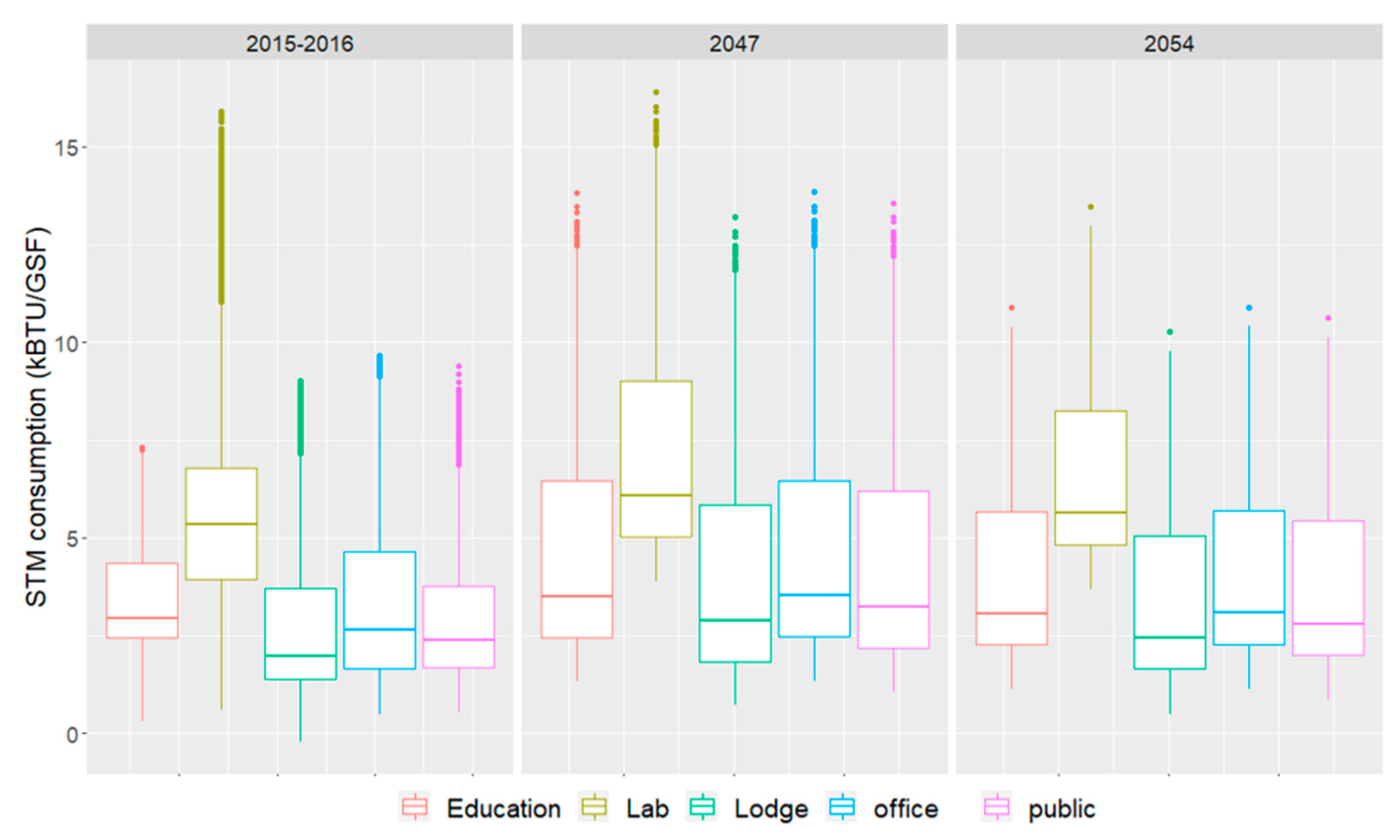
As observed in β coefficient analysis, the weather variable does not influence ELC consumption when STM and CHW are used as another energy source. Based on Figure 6, STM consumption will increase with the humid subtropical climate in both the hottest and coldest scenarios. Climate change will contribute to increasing STM for heating as well as countering the effect of global warming, which can easily be neglected.

5.6. Retro-Commissioning of University Campuses

Universities tend to respond to the challenge of global climate change more effectively as educational institutions compared to other building types. Other building types try to meet the requirements of building energy standards passively and inexpensively when energy policies change. Therefore, checking how universities respond to climate change can be meaningful to glimpse the trajectory for the overall building sector.

When prioritizing and implementing the deferred maintenance program, building operating efficiency and optimization should be fully considered [38]. The monitoring results lead to selecting energy-intensive buildings, which consume more campus energy than other buildings [39]. Based on this selection of the buildings, one should conduct energy audits and retro-commission them. The potential to save energy can be different from the amount of energy consumption. Thus, during the selecting process and retro-commissioning, potential factors that can bring significant change in energy saving need to be examined.

Most energy saving-related information was a prediction, and not actual energy saving results in the energy action plans. These plans tend to be unevaluated, especially when they do not achieve their goal. Universities need to pay attention to actual results by their action plans to use as a reference to evolve energy saving strategies.

Virginia Tech found that 35 percent of all buildings (50 buildings) on campus accounted for over 70 percent of overall university energy costs. Thus, they chose the top ten buildings to focus on energy saving [40]. Boston University reduced its energy consumption by 4% through its energy saving plan after eight years from 2006 while growing in size by 14% [41]. University of Pennsylvania (UPenn) also upgraded lighting in 45 buildings [42]. At UPenn, carbon dioxide equivalent has reduced 32% from STM and 9% from ELC since 2014. Nonetheless, CHW increased 17%, but emitted the lowest carbon dioxide among these three energy types [42].

To save energy, many universities have established energy action plans. Commonly observed action items from 18 universities are shown in

Table 7. Summary of universities’ energy efficiency strategies.

University	The number of LEED Certified Buildings	Energy Efficient Lights	Motion Sensor	Equipment	Window	Geothermal System	Solar Panel	Roof
University of California Irvine	30	Yes					Yes
University of Wisconsin at Oshkosh	6				Yes	Yes	Yes	Yes
Columbia University	7	Yes	Yes			Yes		Yes
Stanford University	4					Yes	Yes	Yes
Washington University St. Louis	21	Yes		Yes			Yes	Yes
UPenn	40	Yes
New York University	11		Yes	Yes
Vanderbilt University	21	Yes			Yes
Quinnipiac University	11	Yes			Yes
Colby College	17						Yes
American University	4 #
Cornell University	26	Yes			Yes
Bentley University	5 *						Yes
Pomona College	10				Yes		Yes	Yes
Iowa State University	22			Yes		Yes
University of Colorado–Boulder	28						Yes
Harvard University	134
University of North Carolina at Chapel Hill	4 #							Yes
Average (Rank)	22	39%	11%	17%	28%	22%	44%	33%

# means that LEED certifications for new construction are required; * means Energy Star certified buildings.

: (1) replacing lights with energy-efficient lights; (2) installing occupancy sensor; (3) equipment reinforcement; (4) upgrading windows; (5) implementing renewable energy system (e.g., solar panels); (6) renovating roofs as green roofs or insulating roofs; and (7) managing building automation (monitoring system).

Table 7 showed that installing solar panels, photovoltaic panels, or solar thermal panels was the most approachable practice, and replacing lights followed next. Improving exterior building shell envelopes was also common practice. This included renovating the roof with a green roof or adding insulation (3rd place) and replacing windows (4th place).

Boston University reduced energy consumption by 2.4 million kWh per year with 8000 LED replacements [41]. Washington University St. Louis upgraded lights with low wattage bulbs, which saved an average of 376,394 kWh per year in energy. Its overall lighting plan has saved more than 20.6 million kWh in total.

Equipment reinforcement includes equipment installation and replacement. Monitoring occupancy behavior is crucial for energy analysis, and installing occupancy sensors can advance operation management. A/C is handled by a centralized chilled water plant system, allowing greater efficiencies [43]. The chiller plant has free cooling capacity that enables universities to reduce energy cost by using the cool ambient air to cool the chilled water. An ice storage system is used for cooling during peak electrical demands. Another method is converting the chiller plant to variable primary flow [39]. It is also beneficial to use economizer ventilation for heat removal [35].

Renovating windows and roofs is one of the most practical renovating methods. Universities can replace single-paned windows with double-paned or triple-paned, thermally efficient glass [35]. Adding insulation during roof replacements or renovating roofs as green roofs is another practical renovation solution.

Implementing a renewable energy system to campus buildings is another energy saving method [41]. The University of Wisconsin at Oshkosh installed solar or photovoltaic panels, which produce 3 million BTUs per day. They provide 70% of the hot water needs for that building with the rate at a total of 47.1 kW, or enough to power four homes. UPenn analyzed its buildings and building systems and determined nine buildings for HVAC and systems replacement.

Leveraging campus building automation systems (BAS) achieves an optimal balance of occupant comfort and energy efficiency through effective building automation and control. A BAS is an integrating component for supply and exhaust fans, pumps, and air handling units, together with components such as flow control valves, air dampers, mixing boxes, instrumentation, thermostats, and humidity control. As a comprehensive monitoring and optimizing system, temperature, pressure, humidity, air balance, and flow rates (both air and water) are controlled to perform effective building occupant safety and comfort and efficient building operation [44]. Additionally, evaluating the feasibility of additional metering during each building renovation project can be implemented [40]. Increasing metering to monitor electricity, steam, and chilled water across campus is beneficial to supervising and managing electrical consumption [35,39,43]. For example, Power Monitoring Expert (PME) software can be used to predict and achieve optimum efficiency [45]. Through BA management, universities can prioritize and identify ways to optimize energy efficiency.

Monitoring temperature control and energy usage throughout the campus saved more than $5 million per year in electricity costs. For example, UPenn used a steam trap testing program over five years and reduced lost steam costs by over 1.2 million dollars [43]. Overall, closely coordinating with facilities services to request and accomplish the prompt repair of building mechanical, electrical, and plumbing systems can bring a difference in energy saving.

6. Discussion

One of the main findings of this research is that there are various perspectives, such as numeric and categorical, to use the same data by forming the data differently. Variables can be in multiple formats depending on research questions, model accuracy, or data availability. For example, when hourly data with date is used, it can be used as (1) timestamp (numeric time with the same interval), (2) categorical variable: periods (categorized by year, month, day, hour, season), type of day, or day of week (3) numeric variable: transformed time considered a periodical feature or time of the day. Another example is that building material that can be used as categorical, binomial, or numeric data. The material itself can be used as categorical data itself, and binomial data can be used when the research focuses on the existence of the material. The other way is quantifying building characteristics, such as the thickness of the wall, density of wall, the thermal conductivity of wall, R-value of the wall, and U-value of the wall. However, since these building characteristics share common elements in their calculation, multicollinearity issues should be handled properly.

Except for the season type for STM, temporal variables are insignificant to estimate energy consumption. Among meteorological variables, the temperature is the solely key variable and expected to increase as evident in STM increase; temperature increase is because of global warming. The developed BEMs showed that the EPD is the most important factor for ELC and the second most important factor for STM consumption. The prediction models give an insight of which factors remain essential and applicable to campus building policy to prevent wasting energy in buildings because of climate change. Therefore, universities need to focus on making action plans accordingly by energy type. For ELC, in order of importance, the vital building variables are EPD, building height, construction year, and U-value of roof. For STM, the vital building variable does not exist.

To predict the future energy use of university campus buildings, derived MLR models were used to estimate energy consumption in 2047 and 2054. In the campus setting, ELC is mainly used for lighting and other appliances, which are barely influenced by the weather. There is significant impact of global warming on building-energy use for heating in the university campus according to prediction result of STM consumption. According to Fan et al. (2014), some independent weather variables, such as the maximum dry-bulb temperature of the prediction day, were used regardless of the BEM methodology [30]. Fan et al. removed these weather variables from all seven different ML methods, although some researchers found that the relative humidity and wind speed are significant [22,23]. Based on CC, partial CC, and relative important inspection, this study’s findings on meteorological variables were aligned with Fan et al.’s findings. On one hand, temperature was the only meteorological predictor, showing significant relevant results with energy consumption for cooling and heating. Meteorological variables except for solar radiation are insignificant to measure ELC. This is because “electricity is used for many more end-uses other than space heating and cooling [46]”. In other words, people use light or other appliances regardless of the weather. On the other hand, temperature above 65 °F is an important variable for STM. It is because STM is used for heating, and CHW is used for cooling in the university campus, unlike residential buildings.

The more variables that are added, the better the explanation that can be made. Therefore, a polynomial regression model with reduced variables was not used, as it had an overfitting problem with variables having a higher power than two. However, a polynomial regression method has merit because it uses only selected variables without the intervention of other minor influential variables.

The developed BEMs showed that the EPD is the second most important factor for STM consumption. However, a low partial CC between EPD and STM was observed, indicating that there is a high indirect impact by other variables related with EPD. Additionally, EPDs of individual buildings are not related to the central controlled boiler for STM. More investigation is necessary for the better explanation of multivariate regression and MLR models.

Universities have saved energy consumption through the renovation of buildings, but building-related variables were not critical based on the developed MLR. This could be because mean WWR was used in this study instead of eastern WWR, western WWR, southern WWR, and northern WWR. Likewise, other building characteristics are averaged values. Additionally, occupancy features and operating variables were inaccessible. This includes building use schedule, heat gain through lights and people, and number of occupants [47]. For more accurate prediction of energy consumption, more variables need to be evaluated.

7. Conclusions

To fight global warming, we need to be aware of the importance of energy saving. In building construction, there are a variety of strategies to reduce building energy consumption. This study used historical data to raise the awareness of people who are linked to this university on the impact of climate change and how to deal with it from a building aspect. The findings can help universities to reduce energy consumption and cost. To answer RQ2, the relationship between input variables and energy consumption by energy types was examined, considering descriptive statistics, relative importance analysis, and BEMs.

This study examined the crucial variables for ELC and STM consumption via statistical analysis methods. In order to explain relationships between variables and energy consumption as well as interpretations of the MLR models, this study analyzed various descriptive statistics. The developed multivariate regression models with different variable sets were analyzed, and stepwise feature selection was used to derive MLR models. For ELC, both multivariate regression models and MLR models suggest that the meteorological variables are insignificant, unlike for STM. The most important four variables out of 22 variables are EPD, building type, building height, and construction year for ELC. These are HD, EPD, building height, and building type for STM.

Among meteorological variables, only the temperature was the outstanding weather variable to estimate STM. EPD was the critical variable for ELC, so universities should focus on EPD when they devise campus energy action plans. Building height was another crucial factor contributing to ELC, so building energy must be considered in the design phase to decide the appropriate building height. The U-value of the roof was critical for ELC. Upgrading windows is regarded as an easy and widespread implementation to boost building energy efficiency. However, the roof needs to be considered as well in order to create an energy-efficient building.

This study observed significant increases in STM consumption in the future (2047 and 2054) in humid subtropical climate zones. The future energy use of university campus buildings needs to be closely monitored as temperature increases due to global warming. Therefore, continuous efforts are required to combat climate change through retro-commissioning by observing and implementing energy retrofit projects based on previous audits. There are many ways that universities can save energy by adopting an energy policy for the campus. For example, they can upgrade chiller programming and investigate the effects of scheduling building fans, increasing set-points, and reducing areas of dehumidification to reduce ELC use. For STM, continuing a steam maintenance program such as replacing steam traps and repairing steam and condensation leaks is the key to energy saving.

One of the limitations of this work was that the sample data was insufficient to categorize by building type. According to Zhai and Helman, a campus-wide analysis of energy use and building characteristics differentiates by building type [31]. That research classified the University of Michigan buildings into laboratories, clinics, service buildings, campus buildings, and residential buildings. Additionally, Amber et al. categorized the campus buildings into administrative buildings or academic buildings [4]. This seems too general to categorize building types, but having two building types can provide a larger sample size for each category. For further research, the sample size should be enlarged to categorize the buildings by building types for a more in-depth analysis. Lastly, more detailed information is required to investigate building renovations because aesthetic improvements or interior renovations do not affect energy consumption.