Structural Health Monitoring of a Brazilian Concrete Bridge for Estimating Specific Dynamic Responses

Abstract

A 3D coupled model to simulate vehicle–bridge interactions (VBI) to estimate its structural responses and impact factors (IMs) was developed in this study. By structural health monitoring (SHM) of a real concrete bridge, several data were collected to calibrate the bridge model by the finite element method (FEM). These models provide the bridge response in terms of vertical displacements and accelerations. VBI models provide reliable outputs without significantly altering the dynamic properties of the bridge. Modified recent analytical equations, which account for the effects of the asymmetric two-axle vehicles, were developed numerically. These equations, plus some proposed solutions, also quantified the vehicle response in terms of accelerations to estimate a more conservative driving comfort. The goal consisted in fitting the SHM with numerical and analytical models to find a more appropriate response for safety purposes and maintenance. From the codes and the literature, it was shown that a unique IM factor was not found. Moreover, most approaches underestimate the phenomena; in fact, results show that a monitored IM factor is 2.5 greater than IM from codes. Proposed equations for vehicle accelerations provided more conservative values up to about three times the standard comfort value.

1. Introduction

The dynamic analyses for bridges under the influence of moving vehicles are of interest for researchers from Bailey’s bridge [1] and the futuristic ultra-high-speed train [2] up to the world’s longest suspension footbridge in 2020 [3,4].

Bridges are subjected to dynamic actions of variable magnitudes due to the different interactions with vehicles [5,6,7,8], humans [9], monorail vehicles [10], and wind vehicles [11].

These interactions affect the behaviour of the bridge and vehicles, particularly the internal stresses of the bridge’s elements and their displacements [12,13,14]. Depending on the magnitude and intensity, these adverse effects may compromise the structural response leading to a reduction in the service life [15].

For concrete bridges, the fatigue behaviour [16] and the pavement imperfection effects by analytical and numerical solutions [17,18] and experimental tests [19,20] were studied. For steel bridges, several conventional solutions [21,22,23] or modular solutions [24,25] were proposed.

In order to quantify the response of the bridge under moving vehicle actions, there are several methods. These problems are usually treated by using the vehicle–bridge interaction (VBI) models.

In [26,27], four basic VBI models are shown, from the simpler moving vertical load or mass model to the more complete sprung mass and suspended rigid beam model. These models provide analytical solutions to be used for preliminary and reference results.

More recently, some modified VBI analytical models were proposed. In [28], the modified, suspended rigid beam model considers the asymmetrical two-axle vehicle to account for the different vertical actions of the vehicle weight acting on the bridge. In [29], the same model was modified, adding an elastic foundation of the bridge to detect its possible damage.

However, analytical models are subjected to some approximations neglecting some effects, e.g., the irregularity of pavement [11,12] and the continuous interaction vehicle–bridge point-by-point [30,31].

For this, more advanced methods that account for these effects were developed. In [7,32], numerical models based on a coupled multibody finite element method (MB-FEM) are shown [33,34]. In [35], an alternative numerical model was proposed where the bridge was schematised by a single-line model. These methods are usually developed by the Runge–Kutta approach explicating the time marching scheme [36,37].

Other advanced numerical solutions to provide a more precise VBI model were proposed in [38] and [39], where an arbitrary Lagrangian–Eulerian approach by adopting a fixed coordinate system is proposed. In [11,40], specific approaches to study the wind effects were presented by a complete wind–VBI framework.

The main goals of these models are basically to estimate: (i) the dynamic amplification of the bridge and (ii) the vertical accelerations of the vehicle. Both goals account for the vertical actions of the moving vehicle that act on the bridge amplifying the static behaviour of the system of a certain factor called “dynamic amplification factor (DAF)”, “dynamic load allowance (DLA)” or—used in this paper—“impact factor (IM)” [31,41,42].

The common practice consists in multiplying the calculated IM factor by the static forces, internal stresses, and displacements [43] and thus developing the pseudo-static verifications of the bridge.

There are several equations in codes and manuals to obtain IM factors, as shown in [44,45]. The key parameters more used are the span length and the frequency of the bridge. Most formulas are calculated by the span length, and they are calibrated by experimental tests, e.g., American [5,46,47], English [48], Brazilian [49], Italian [50], and Portuguese [51] codes. In [42], it was stated that “these formulas yield inconsistent results that can differ widely”.

In [52], it was shown, by analysing 256 bridges, that the IM factors calculated using only the span length underestimate the dynamic amplification as a parameter; for this, it was suggested to consider the bridge frequency parameter.

In general, several design codes would underestimate the IM factor for standard road surface [53] and under poor road surface conditions [30]. However, many parameters are often neglected also in the VBI analysis, e.g., braking and accelerations/decelerations of the vehicles, type of bridge, axle load, and traffic tonnage [45].

Some advanced codes, e.g., European [54] and Spanish [55], account for not only the bridge span length but also its structural behaviour and vehicle speed. The pavement status is also considered; however, it is considered by a simple coefficient, so the continuous interaction vehicle–bridge, above mentioned, is completely neglected.

Due to the road surface deterioration of existing bridges, some studies showed that the real IM factors could be higher than the values indicated in codes and manuals, which refer to new bridges [5,30,45,56]. Regarding the vehicle speed, as a parameter to define IM factors, in [30], it is mentioned that “an increase of vehicle speed does not necessarily guarantee an increase of the impact factor” as also shown in [18,20].

In [57], it was concluded that the IM factor of the bending moment is higher than that of deflection when the bridge deck is deteriorated, reaching a value of 0.70; in [34], it can reach up to 0.90 if the road surface irregularities in the lateral direction are neglected. However, it was demonstrated that it is very difficult to estimate by a unique form of the IM factor. In [53], it is stated that the determination of the IM factor “remains as a controversial issue”.

For this, in the past three decades, significant efforts to investigate the IM factors have been carried out by using several models accounting for not only the above-mentioned parameters but also vehicle weight, vehicle position, high vibration modes [17,18,57], 3D pavement irregularities [11], and the road surface in lateral directions [19,30]. In [53], alternative effects on the IM factors due to the skew angle of the bridge were also included.

Due to the several randomnesses present in these analyses, many studies adopt probabilistic methods, as shown in [43,45,56]. In fact, in [45], it was concluded that IM factors by deterministic analysis “cover only 1.14% of the real estimation”.

Finally, as mentioned in [52], “an exact impact factors can be obtained by measuring the response under in-service conditions”; however, in [38], it is “complicated to analyse vehicle–bridge interaction dynamics” in “real-life situations” since there are several factors that affect the whole system and “their whole coverage in the literature is limited”. Moreover, in [56], it is mentioned that the actions and responses of the system “cannot be exactly known because of the inherent uncertainty affecting them”.

All these considerations should represent the motivations and justifications of this study.

In this paper, the real behaviour of a Brazilian bridge was monitored by structural health monitoring (SHM) analysis, which is currently considered the best analysis [58]. Analytical and numerical solutions of VBI models were carried out to study the bridge and vehicle responses for several conditions. All these analyses should reach a high precision level to obtain more realistic results for safety purposes and maintenance of bridges, which is also explained in [58].

2. Case Study

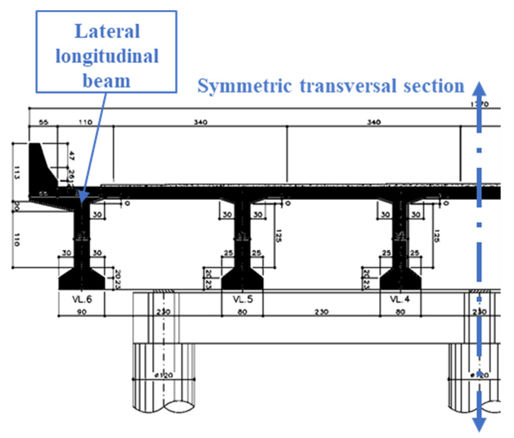
2.1. Brazilian Concrete Bridge

The case study is the simply supported bridge placed at São Paulo State in Brazil. Figure 1 shows a photo of the bridge (with the position of the monitoring devices T1, T2, and A) and its FEM model [59,60,61]. Figure 2 shows the technical drawing of the symmetric transversal section of the bridge [62]. The FEM model of the lateral longitudinal beam is also shown in Figure 1b since it represents the beam where the T1 sensor is placed. It is called “equivalent beam”, as explained in Section 2.4.

The bridge was modelled using Sap2000 software (Computers and Structures, Berkeley, CA, USA) [60]. The 3D model was formed by four longitudinal central girders; two longitudinal, lateral girders; three transversal central beams; two transversal lateral beams; one slab composed of shell elements (0.50 m × 0.50 m); and six foundation piles connected to the super-structure by six elastomeric pads modelled as “rigid link”.

At the end of the pile was assigned a vertical translation restrain, and along the pile was assigned a horizontal spring value of 5000.0 kN/m to simulate the horizontal confinement of the ground with the pile [43].

The model was constructed in an attempt to reproduce the real structure in a better way; thus, the axis of each bar coincided with its centre of gravity, the nodes of the slab coincided with the nodes of the beams, and the dead weight of each element was manually inserted to avoid the double calculation in the overlapped sections.

The permanent loadings consisted of the dead weight of the structural and non-structural elements, pavement weight, and wheel-guard weight.

Table 1. Bridge data.

Parameter	Value
Longitudinal length, L	41.90 m
Transversal length, D	17.70 m
Pile length	15.0 m
Pavement weight	24.0 kN/m3 a
Wheel-guard weight	7.85 kN/m3 b
Bridge mass, mb	8500.95 kN
Bridge frequency, fb	2.421 Hz c
Bridge damping ratio	5.0% [49]
Horizontal stiffness of one elastomeric pad	24,000.0 kN/m d
Concrete elastic modulus, E	50.0 GPa d
Concrete transversal modulus, G	23.0 GPa

^a This loading was applied on the trail surface of 0.10 m. ^b This loading was applied for a width of 1.0 m. ^c This value refers to the fourth mode where the modal participating mass ratio (MPMR) is predominant in the vertical direction (MPMR = 63.57%). ^d Values provided by the designer.

shows the geometrical parameters and loadings of the studied bridge.

In the literature [16,52,63], there are several relations to estimate f_b in the function of L. From these studies, a mean value of f_b = 2.76 Hz was obtained (for the studied bridge), which is similar to the 2.421 Hz used in this analysis. These relations were calibrated by monitoring real bridges in different countries; therefore, they can be used only as general reference values.

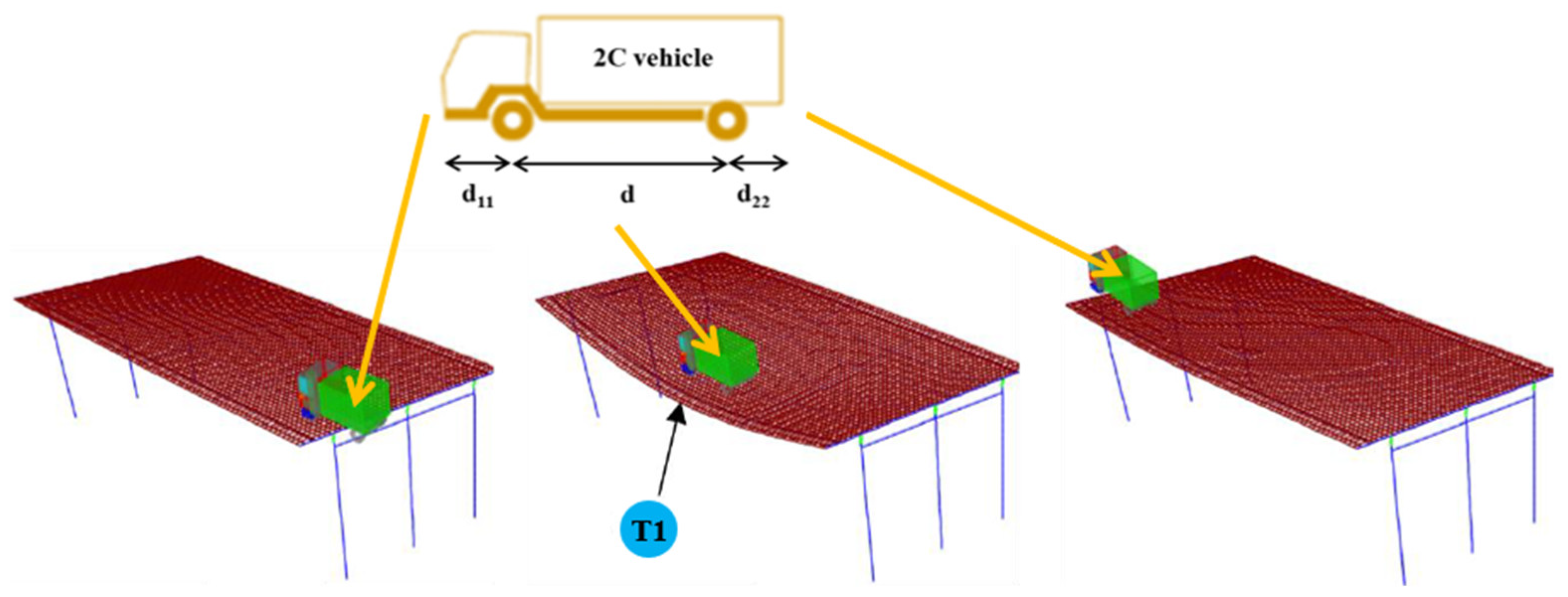
2.2. Vehicle Loadings

This vehicle, called the “2C vehicle”, represents the most common vehicle that circulates on Brazil’s roadways, with a quantity on the road of 26.0%, as indicated in [56]. In this sense, it could represent the vehicle “used” for “in-situ” experimental testing.

The configuration of the used two-axle vehicle indicating the predefined lengths, i.e., the distance between both wheels, d, and the distance from the front wheel, d₁₁, or rear wheel, d₂₂, of a car to its nearest end, is shown in Section 2.3.

Table 2. The 2C vehicle data.

Parameter	Value
Vehicle mass, mv	15,000.0 kg a
Front suspended mass, mv,1	772.0 kg a
Rear suspended mass, mv,2	1066.0 kg a
Length d11	0.50 m [56]
Length d	4.50 m [56]
Length d22	2.0 m [56]
Front suspended frequency, fv,1	3.71 Hz b
Rear suspended frequency, fv,2	6.86 Hz b
Front suspended stiffness, k1	580.0 kN/m [35]
Rear suspended stiffness, k2	1180.0 kN/m [35]
Vehicle frequency, fv	2.41 Hz c
Mass moment of inertia, Jc	~25,000.0 kg m2

^a Estimated by the influence line (Figure 3). A weight of 15,000 kg was distributed as 6300.0 kg (front) and 8700.0 kg (rear). ^b Estimated values from the literature [35]. ^c It refers to the vertical pitching movement. It was estimated by using two spring in series with k_v,eq = 388.86 kN/m and m_v,eq = 17.01 kN. This value is consistent with the literature, e.g., 2.30 Hz [15,32] and 2.46 Hz [42].

lists the used data regarding this vehicle. The considered vehicle speed is v = 16.0 m/s (≈60.0 km/h) since it represents the mean speed registered to assume a stationary traffic action during the monitoring period.

In a more complete model, the contribution of the wheel should be considered [34,35,38]. However, the suspended system (i.e., vehicle suspensions k₁, k₂) is predominant in terms of the frequency with respect to the non-suspended system (i.e., tires) of ~7 times, as shown in the literature [18,29]; therefore, in this study, the parameters m_v and f_v can adequately represent the whole vehicle system.

The transverse load distribution of the vehicle (one axis) was performed according to the Fauchart’s method, where the girders are replaced by translational (k_b1 and k_b2) and rotational (k_θ1 and k_θ2) spring constants, then connected to a longitudinal slab strip of 1.0 m width, as described in [16,64].

By using this method, the VBI analytical analyses should consider the influence of the transverse location of the vehicle on the bridge. Figure 3 shows the scheme of Fauchart’s method and the influence line developed by the Ftool software [65].

In this method, the Euler–Bernoulli beam model was applied to the girders. The constant springs were determined by the beam equation for bending and torsion and through a Fourier’s expansion. They are estimated as [64]:

$$\left\{\begin{array}{cc}{k}_{bi}=E{I}_i{\left(\frac{\pi }{L}\right)}^4& \to \left\{k_{b1}=1008.0;k_{b2}=1092.0\right\}kN/m\\ k_{\theta i}=G{J}_i{\left(\frac{\pi }{L}\right)}^2& \to \left\{J_1=23.41;J_2=25.96\right\}{m}^4\to \left\{k_{\theta 1}=3071.0;k_{\theta 2}=3406.0\right\}kNm/rad \end{array}\right.$$

(1)

where E, G and L were defined in Table 1; I and J are the moment of inertia (

Table 3. Equivalent longitudinal beam data.

Equivalent Parameter	Value
Concrete elastic modulus × inertia, (EI)eq	1.94 × (50.0 GPa × 0.7255 m4) = 70.37 GN m2 a
Mass, mb,eq	6714.34 kg/m b
Longitudinal length, Leq	42.0 m c
Frequency, fb,eq	2.40 Hz c

^a The inertia I = 0.7255 m⁴ and the mass m_b = 3461.0 kg/m refer to the external longitudinal beam shown in Figure 1b and Figure 2. ^b Estimated as ratio between the total vertical reactions in the external supports due to the permanent loadings and L_eq. ^c The same values of the whole bridge are used due to calibration by the factor 1.94 (see Table 1).

) and torsional inertia of the beam, respectively.

From the influence line we obtained m_v,1 = 772.0 kg (≈30.90 (0.18 + 0.065)) and m_v,2 = 1066.0 kg (≈42.70 (0.18 + 0.065)) (Table 2). These values are consistent with the literature [35,56].

2.3. Structural Health Monitoring (SHM)

The structural health monitoring of the Brazilian bridge lasted 8 months, and it consisted of three phases: (i) registration of the structure data (usually accelerations [58]), (ii) elaboration and transmission of data and (iii) visualisations and plotting of the output data.

The registration of the data was made by the accelerometer “ADXL355” (points T1 and T2 as already shown in Figure 1a), which records the accelerations of the bridge in the three directions, with the radio frequency component “NRF24L01” and the microcontroller “Arduino NANO” (Figure 4a). In this study, only the vertical accelerations were treated.

For the elaboration and transmission of data, the same accelerometer and “NRF24L01” device were used with the “Arduino NANO” device for the transmission, and the micro-computer “Raspberry Pi 4B” (see point A in Figure 1a) and microcontrollers “Arduino UNO” (Figure 4b) device for the elaboration/visualisation.

A fast Fourier transform (FFT) was implemented by the microcomputer to detect the high Fourier amplitude of the bridge to monitor the possible variation in the bridge behaviour. Collected data were sent by 4G mobile phones each ~2.0 min to a predefined cloud [66].

Finally, all accelerations were visualised by a “dashboard” developed in “Python” language. In [66], it was possible to see in real-time the monitoring of the bridge and its structural 3D model.

Figure 5 shows the non-adjusted registered vertical accelerations (~10⁴ registrations) by the T1 and T2 sensors. The used maximum value is 7.98 m/s² (see Section 4.1).

During the long monitoring, several accelerations were registered; therefore, some choices were made to select the more useful accelerations. The criteria mainly regard the amplitude of the accelerations and the sharpness of the signal concerning the noise interferences. For this, the accelerations were filtered by PRISM software [67], applying the low-pass filter with a cut frequency of 0.20–25.0 Hz using an 8-th order Butterworth filter [40]. Moreover, the accelerograms were corrected using the baseline correction to remove large errors in the velocities and displacement records caused by double time-integration [68].

Another aspect regarding the vibrations during the entering of the vehicle on the bridge. In fact, the bridge is fixed to the road by mechanical joints that can generate large vertical accelerations that must not be considered [11,35]. The free vibrations caused by all previous loads passing the considered beam were also suppressed (e.g., other vehicles, human-induced vibrations).

From the FEM model, the estimation of the vertical acceleration was also calculated. Due to the difficulty in simulating the real phenomenon well, 78 cases with several-speed v and m_v of the vehicle were generated. These cases allow calibrating the model to obtain good results. Figure 6 shows the steps of the 2C moving vehicle on the bridge. In order to obtain consistent results concerning the real monitoring, the same T1 point was used as a reference point. The results are shown in Section 4.

2.4. Definition of the Equivalent Beam

In order to develop the VBI model by analytical solutions, it is necessary to define an equivalent beam. The equivalent bending stiffness of the beam that provides equivalent vibration modes concerning the whole structure must be estimated [35]. For this, a concentrated load of 10.0 kN was applied in the middle of the longitudinal beam of the FEM model. From the obtained vertical displacement (=0.209 mm), by classical beam theory, an equivalent EI, (EI)_eq, was estimated. Thus, a factor, defined as a ratio between the real value and the equivalent value, was found (=1.94).

This factor of 1.94 should allow a good agreement between the whole bridge and its equivalent beam; thus, some parameters (i.e., L_eq, f_b,eq) of the equivalent beam are the same as for the whole bridge. Table 3 shows the data of the adopted equivalent beam.

Once the parameters for an equivalent beam were found, it was necessary to define a model to extrapolate the results to determine the IM factors. In the following sections, two analytical models were used to obtain dynamic displacements of the bridge, thus the IM factors. Moreover, the vehicle response was estimated.

3. VBI System

3.1. Modified Suspended Rigid BEAM Model

The suspended rigid beam model is based on the application of two concentrated loads to a simple-supported beam following the Euler–Bernoulli theory [26], as shown in Figure 7. The system was modelled with four degrees of freedom (DOFs) (three verticals u₁, u₂, y, and one rotational angle θ) and two suspended stiffnesses k₁ (front) and k₂ (rear).

Only one car was accepted to move on the bridge with constant velocity v, and the vehicle wheels were always in contact with the bridge surface during the crossing, and no jumps occurred [34,38]. For short/medium span bridges (i.e., L < 40.0 m [69]), this hypothesis of a reduced number of vehicles (here one vehicle) should represent the more critical situation as explained in [58,63].

The modified suspended rigid beam model, introduced in [32] and improved in [28], consists of accounting for the asymmetric of the vehicle, which could represent a real situation. In fact, the used 2C vehicle is subjected to an asymmetrical interaction with the bridge since d₁ = 2.61 m > d₂ = 1.89 m.

This model neglects the damping of the vehicle and bridge and does not account for the pavement irregularity between the two bridge/vehicle contact points [70]. In the literature, it was shown that the contribution of vehicle [32] and bridge damping [17,63] could play a minor role in the dynamic amplification of the bridge.

3.1.1. Bridge Response

The equation of the motion of the beam is [28]:

$$m_{b,eq}\ddot{u}\left(x,t\right)+{\left(EI\right)}_{eq}u{\left(x,t\right)}^{⁗}=F\left(t\right)$$

(2)

where m_b,eq is the mass of the equivalent beam per unite length, (EI)_eq is the equivalent elastic modulus times the moment of inertia, and u(x,t) is the vertical displacement of the beam. The superscripts (′) and (˙) denote differentiation concerning the horizontal axis x and time t, respectively.

Given that vehicle mass m_v is very small compared with the bridge mass m_b (here m_v/m_b = 0.017 < 0.30 [53]), the vehicle’s action on the bridge can be treated as two external discrete moving loads (k = 1, 2) neglecting the VBI effects:

$$F\left(t\right)={{\displaystyle \sum }}_{k=1}^2{p}_k\delta \left[x-v\left(t-t_k\right)\right]\left[H\left(t-t_k\right)-H\left(t-t_k-\Delta t\right)\right]$$

(3)

where δ is the Dirac delta function, H is the unit step function, v is the vehicle velocity. Other parameters are: $\Delta t=\frac{L_{eq}}{v}$, $p_k=\frac{d-d_k}{d}(m_v g)$, $t_k=\frac{\left(k-1\right)d}{v}$, where L_eq is the equivalent length of the beam, d is the vehicle length, d_k is the distance from the k-th axle to the centre of gravity, g, of the vehicle.

The displacement of the simple supported beam is described by [71]:

$$u\left(x,t\right)={\varphi }_n\left(x\right)q_n\left(t\right)\to u\left(x,t\right)={{\displaystyle \sum }}_{n=1}^N\left[q_n\left(t\right)sin\left(\frac{n \pi x}{L_{eq}}\right)\right]$$

(4)

where ϕ_n(x) denotes the n-th vibration mode, q_n(t) denotes the modal generalised coordinates, x = v(t − t_k), N = 1.0.

By substituting Equations (3) and (4) in Equation (2), multiplying both sides of the equation by sin[(nπx)/L_eq], and integrating for L_eq, the following was obtained:

$${\ddot{q}}_n\left(t\right)+{\omega }_{bn,eq}^2 q_n\left(t\right)=F_n\left(t\right)$$

(5)

where ω_bn,eq is the equivalent circular frequency and F_n(t) (see Equation (3)) is defined as:

$$F_n\left(t\right)=\frac{2}{m_{b,eq} L_{eq}}{{\displaystyle \sum }}_{k=1}^2{p}_k\left[sin\left(\frac{n \pi v\left(t-t_k\right)}{L_{eq}}\right)H\left(t-t_k\right)+{\left(-1\right)}^{n+1}sin\left(\frac{n \pi v\left(t-t_k-\Delta t\right)}{L_{eq}}\right)-H\left(t-t_k-\Delta t\right)\right]$$

(6)

Obtaining q_n(t) by solving Equation (5) for q_n(0) = 0 and ${\dot{q}}_n$(0) = 0, Equation (4) becomes:

$$\begin{gathered} u\left(x,t\right)={{\displaystyle \sum }}_{n=1}^N{{\displaystyle \sum }}_{k=1}^2{A}_n{p}_k\left\{\left[sin\left(\frac{n \pi v\left(t-t_k\right)}{L_{eq}}\right)-S_n\sin \left({\omega }_{bn,eq}\left(t-t_k\right)\right)\right]H\left(t-t_k\right)+\left[sin\left(\frac{n \pi v\left(t-t_k-\Delta t\right)}{L_{eq}}\right)- \\ {S}_n\sin \left({\omega }_{bn,eq}\left(t-t_k-\Delta t\right)\right)\right]H\left(t-t_k-\Delta t\right)\right\}sin\left(\frac{n \pi x}{L_{eq}}\right) \end{gathered}$$

(7)

where $A_n=-\frac{2L_{eq}^3}{{\left(EI\right)}_{eq}{n}^4{\pi }^4\left(1-S_n^2\right)}$ and $S_n=\frac{n\pi v}{L_{eq}\times {\omega }_{bn,eq}}$.

3.1.2. Vehicle Response

The governing equations of the motion for the vertical displacement y(t) and rotational angle θ(t) of the vehicle can be defined with respect to the static equilibrium position. These equilibriums are [28]:

$$\left\{\begin{array}{c}{m}_v\ddot{y}\left(t\right)+k_1\left(y\left(t\right)+d_1\theta \left(t\right)-u_1\left(t\right)\right)+k_2\left(y\left(t\right)-d_2\theta \left(t\right)-u_2\left(t\right)\right)=0\\ J_c\ddot{\theta }\left(t\right)+k_1{d}_1\left(y\left(t\right)+d_1\theta \left(t\right)-u_1\left(t\right)\right)-k_2{d}_2\left(y\left(t\right)-d_2\theta \left(t\right)-u_2\left(t\right)\right)=0\end{array}\right.$$

(8)

where J_c is the mass moment of inertia of the vehicle, whereas the other parameters were already explained.

As mentioned in [28,29], the vehicle response is quite complicated to be found analytically since the wheel responses u₁ and u₂ are “a-priori” unknown. However, it is possible to define some functions for u₁ and u₂ as input signals for two wheels. In this way, by substituting u₁ and u₂ in Equation (8), with the initial conditions y(0) = 0 and y′(0) = 0, it is possible to estimate y and θ. Possible relations proposed by the authors are shown in Section 3.3.1.

3.2. Sprung Mass Model

This VBI model is based on the simply supported beam subjected to a moving sprung mass where the vehicle (or sprung) mass m_v is supported by a dashpot–spring unit of spring constant k_v [26,27]. The above-mentioned hypotheses explained for the suspended rigid beam model are still valid for the sprung model.

The system was modelled with 2-DOFs (i.e., the vertical displacements y and u), and a unique contact point between vehicle and bridge was present, as shown in Figure 8.

The equation of the motion of the beam and the vehicle are given by, respectively [26]:

$$\begin{gathered} \ddot{u}\left(t\right)+\left(2{\omega }_v^2\frac{m_v}{m_{b,eq} L_{eq}}\sin {\left(\frac{\pi v t}{L_{eq}}\right)}^2+{\omega }_{b,eq}^2\right)u\left(t\right)-\left(2{\omega }_v^2\frac{m_v}{m_{b,eq} L_{eq}}\sin \left(\frac{\pi v t}{L_{eq}}\right)\right)y\left(t\right) \\ =-2\frac{m_v g}{m_{b,eq} L_{eq}}\sin \left(\frac{\pi v t}{L_{eq}}\right) \end{gathered}$$

(9)

$$\ddot{y}\left(t\right)-\left({\omega }_v^2\frac{m_v}{m_{b,eq} L_{eq}}\sin \left(\frac{\pi v t}{L_{eq}}\right)\right)u\left(t\right)+{\omega }_v^2 y\left(t\right)=0$$

(10)

In this form, Equations (9) and (10) refer only to the first vibration mode of the beam ϕ₁(x) (see Equation (4)).

The vertical deformation, u(t), at the beam midpoint was obtained by solving the system of Equations (9) and (10) under u(0) = 0 and $\dot{u}$(0) = 0; thus, $\ddot{y}\left(t\right)$ was also found.

3.3. Additional Effects for VBI

The described analytical VBI models have the great advantage of solving a relatively simple problem regarding the bridge response under vehicle moving providing good results for bridge design. However, as mentioned in Equation (3), the VBI effects, due to continuous interaction between vehicle and bridge, were not considered.

Usually, these effects amplify two main actions that can destabilise the vehicle and the passengers, i.e., the vehicle vertical accelerations, which are directly correlated to the riding comfort, and the pavement irregularities, which produce additional dynamic forces by exciting vehicle mass that impact on the bridge slightly destabilising the riding comfort.

3.3.1. Vehicle Vertical Accelerations

The vehicle vertical accelerations of the sprung mass model serve as a measure of the riding comfort for passengers [26]; moreover, in [27], it was stated that “the acceleration of the sprung mass has been taken as a measure of the passengers’ riding comfort”.

By developing Equation (10), it is possible to estimate a possible trend of the vehicle vertical accelerations, which can be used as a reference model. Therefore, by adopting simple cosine harmonic functions, u₁ and u₂ (see Equation (8)), as input signals to the two wheels as suggested in [28], it could be possible to estimate the vehicle vertical accelerations by using the suspended rigid beam model.

The process is iterative since the functions u₁ and u₂ were adopted “a-priori”, and their amplitude U₁ and U₂ are unknown. The authors propose the following relations to directly find a possible vertical response of the vehicle:

$$\left\{\begin{array}{c}{u}_1\left(t\right)=U_1\cos \left({\omega }_{v,1}t\right)\\ u_2\left(t\right)=U_2\cos \left({\omega }_{v,2}t\right)\\ U_i=\frac{m_{v,i}\times g}{k_i}\end{array}\right.$$

(11)

The criterium of the proposed Equation (11) follows the principle used in [28] in adopting cosine function but here m_v,I; thus, U_i are estimated by using Fauchart’s model. In this sense, both models (i.e., suspended + Fauchart) were coupled to provide new solutions.

In this analysis, from Table 2, both amplitudes are U₁ = 18.03 mm and U₂ = 5.28 mm, but for other cases, these amplitudes should be quantified by a function of the considered vehicle. Figure 9 shows the response of the vehicle suspensions in t by Equation (11) [71]. Provided that k₁ < k₂, it is necessary for a great displacement u₁ to equilibrate the system.

3.3.2. Pavement Irregularities

For pavement irregularities, the road/wheel roughness is usually considered as indicated in the literature [30,34,42,72]. However, there are two other types of irregularities: (i) the manufacturing imperfections corresponding to initial deformations of the pavement modulus (more common for steel pavements), and (ii) the installation misalignments correlated to vertical step defects in the transversal joints of pavement modules [63,70].

In this study, the irregularity effects in the analytical and FEM analyses are not considered for two main reasons (it is clear that for experimental results, they are intrinsically considered; however, it is difficult to quantify their contributions):

(1)

The contribution of the IM factors due to irregularities could be low. When considering three imperfections, in [70], it was shown as the total 2D irregularities are about ±4.0 mm. In [11], a more accurate analysis by considering 3D pavement irregularities was carried out, estimating an amplitude of about ±5.0 mm. In [38,39], it was shown that the irregularities affect the vertical bridge displacements little; in fact, the response obtained accounting for the irregularities is very similar to the analytical solutions without irregularities. However, for larger amplitude (e.g., > ±15.0 mm), the irregularity effects should not be neglected, as shown in [12]. In [34], road surface irregularities in the lateral directions can quite amplify the IM factor;

(2)

Most codes do not explicitly account for the irregularities; therefore, they are not considered in design practice for bridges. Codes provide equations and methods for new bridges where the pavement is considered of a very good quality and under standard maintenance (i.e., class A [72]). The irregularities are considered in, e.g., Spanish code [28] and European code [54] using a factor between 0.50 and 1.0, and in the literature [30], where is proposed a factor between 0.70 and 6.0. However, in [28,54], the irregularity contribution on the IM factors is very small, e.g., for the studied bridge, it is 0.42%.

3.4. IM Factor

The IM factors are evaluated based on the following Equation (12) [70]:

$$\mathrm{IM}=\left(\frac{u\left(t\right)}{u}-1\right)$$

(12)

where u(t) and u are the dynamic and static vertical bridge displacement, respectively, already defined.

Equation (12) defines the IM factors through a ratio in which the static quantity is magnified to obtain the dynamic quantity by using numerical methods. Several predefined methods exist to estimate the IM factors, as listed in

Table 4. Some approaches for estimating the IM factors.

Reference	Specification for IM Factors
Codes and manuals
American (AASHTO) [47]	It amplifies static live load stresses. It is estimated by L. IM < 0.30–0.33 a
American (AREA) [5]	It is estimated by L and D
Brazilian (NBR) [49]	It amplifies static vertical moving loads. It is estimated by L. IM < 0.35 b
English (BS5400) [48]	It amplifies static bending moments and shears. It is estimated by L. IM < 1.0
Italian (NTC) [50]	It amplifies static stresses and displacements. It is estimated by L. IM < 1.0
Portuguese (RSA) [51]	It amplifies static loads and transversal forces. It is estimated by L. IM < 1.0
Spanish (IAPF) [55]	It amplifies static forces. It is estimated by L, v, fb
European (Eurocode) [54]	It amplifies static forces and moments. It is estimated by L, v, fb
Canadian (CSA) [41]	It amplifies static live loads. It is estimated by fb and the number of axles. IM < 0.40
Published studies
Deng and Cai (2010) [30]	It is estimated by L and pavement irregularities. IM < 0.33 a
Rodrigues et al. (2013) [56]	It is estimated by L, v, fb
Carneiro et al. (2021) [16]	It is estimated by L, v, fb
This study	It was defined by “in-situ” experimental tests, FEM and analytic VBI models

^a Adapted from [46]. ^b For the studied bridge, the previous Brazilian code reduced the IM by 0.48% [56].

. Other methods are shown in [52,45], where two types of IMs are listed: one regards the vehicle and the other the bridge.

Most of IM factors are calibrated for concrete bridge with relatively medium span (e.g., L < 65.0 m [48,52]) and for train actions [7,30] (experimental approach). The main three parameters used for the IM estimation are L (geometrical approach), and f_b and v (dynamic approach).

It is interesting to note that the Canadian code [41] associates f_b with the number of axles, which can be correlated to the transversal length of the bridge D, also studied in the AREA American manual [5,63]. These relations could account for the transverse location of the vehicle on the bridge; however, it is difficult to quantify it.

In [5,31] was reported that a unique safe IM factor could not guarantee the safe evaluation of the whole bridge; therefore, local analyses of the structural and non-structural elements are necessary.

4. Analyses and Results

4.1. Calibration and Some Structural Responses

The calibration consists in fitting the maximum bridge accelerations due to the vehicle moving provided by the four explained analyses: (i) “in-situ” experimental measurements, (ii) FEM model; (iii) suspended model; (iv) sprung model.

The used parameters are shown in Table 1, Table 2 and Table 3 with v = 16.0 m/s (= 57.60 km/h). This value was chosen since, as stated in [42], “in most cases the DAF of a continuous beam bridge peaks at the velocity range of 40–60 km/h”.

In a similar way to [73], both analytical models are used to verify the accuracy and efficiency of the experimental tests and FEM model.

In order to homogenise the horizontal axis, some step numbers (0–3.69) were defined where each accelerogram is formed by 209 points. With Δt = 2.62 s (defined in Equation (3)) each step is equivalent to 0.71 s. Figure 10a shows the response of the bridge in terms of accelerations by using all models with the vehicle entering the L span of the bridge. The numerical analyses were carried out by Mathematica software [74].

In Figure 10a, the registered acceleration (blue points) is considered an exact solution where all external and internal interactions of the system are included. The FEM acceleration (black line) is intrinsically an approximation influenced by modelling conditions; however, it provided good results. Both analytical suspended and sprung models (red lines) could also represent exact solutions, but under some specific approximations (already mentioned); in fact, they provided more regular trends with low frequencies with respect to the other results.

As known, the peak accelerations do not happen in the midpoint of the beam due to the interlocking effect of the front and rear wheels [27]. This effect moves the acceleration trends towards the vehicle direction. The acceleration peak values of the sprung and suspended model are 8.56 m/s² and 8.25 m/s², respectively, whereas the registered and FEM accelerations provide a peak value of 7.98 m/s² (i.e., 0.814 g, see Figure 11) and 8.86 m/s², respectively. These values show a good correspondence between all models (the coincidence of points in Figure 10a).

The difference between analytical responses and other ones can be attributed mainly due to the omission of higher modes; in fact, the analytic results only consider the first vibration mode of the bridge [27]. In [19], it is shown as numerical solutions can provide higher values than experimental solutions. However, considering only the first vibration mode can be considered acceptable, as shown in [53].

Moreover, the VBI results by the FEM model and experimental tests account for the transverse location of the vehicle in the bridge; however, it is difficult to estimate its real percentage. In the analytical VBI analyses, these should be considered by coupling Fauchart’s method with the suspended model.

FEM results show very low vertical accelerations in the interval 0.5–2.0 s due to probably a damped response of the bridge that is not excited by the vehicle. Other differences can be attributed to the non-linear effects of the material and damping ratio, which are only accounted for in the registered results.

If all analytical and numerical displacements can be directly calculated for the registered displacement, it is necessary to discuss some aspects. As mentioned in Figure 5, the real selected accelerogram was filtered and then corrected. However, this does not imply that the choice of the adequate displacement is direct; in fact, the maximum acceleration corresponds to the maximum displacement of 7.627 mm, which is 1.85 times the static value (i.e., 4.12 mm) calculated by the FEM model [60]. This means that the IM calculated by Equation (12) would assume a very high value (i.e., IM = 0.85); therefore, it could be reasonable to consider a group of dynamic displacements and to use its mean value.

However, it is important to highlight that in the literature, high values of IM are found; for example, in [56], by experimental measurement, a maximum value of IM = 0.84 was registered, whereas in [39], a numerical value of IM = 0.70 is estimated. By probabilistic analyses, IM could also reach a value of 0.88 [45], up to 0.90, when the road surface irregularities in the lateral direction are neglected [34].

Figure 11 shows the real accelerogram (already shown in Figure 10a) in a very short interval where three peaks are included. The criterium consists in selecting the values of the dynamic displacements (red curve)—obtained by integrating the real accelerograms by PRISM software [67]—greater than the static displacement (horizontal line) obtained by the FEM model and then defining their mean value, i.e., 6.04 mm.

Other maximum displacements are 5.96 mm, 4.86 mm and 6.26 mm for FEM, sprung and suspended models, respectively (see Figure 10b).

4.2. Other Structural Responses

Other analyses to estimate the dynamic responses of the bridge by varying the vehicle speed v between v ≈ 20.0 and 120.0 km/h were carried out. These speed values are expected in the road traffic for the studied bridge. Figure 12 shows only some cases. The values by registered and FEM model refer to v = 16.0 m/s (≈60.0 km/h)

The considerations of Figure 10 are still valid for Figure 12. By changing the vehicle speed v, it is possible to note that the maximum bridge displacements are not much altered, and they maintain at ~4.5 mm and ~6.0 mm for the sprung and suspended model, respectively; however, it alters the trend of the curve due to the variation in the sin(·) function in both models (see Equations (7) and (9)). The main parameter that changes both responses is ω_b,eq; in Equation (9), this parameter is also squared.

This effect is more evident for the accelerations since they are calculated by deriving two times u(t). Moreover, by plotting ü(t) curves, the effects of vehicle speed v are more evident.

In general, the vertical accelerations of the bridge increase with the increase in the vehicle speed in accordance with the literature [6,8]. For v between 11.0 and 16.0 m/s, similar trends of vertical accelerations of the bridge are verified, indicating that both models can be valid for this range.

However, as mentioned, these analytical models do not account for the continuous interaction between vehicle and bridge, which can increase bridge displacements. Physically, as mentioned in [53], it is possible that, at high v, there is insufficient time for the force to compel a significant dynamic deflection in the bridge; thus, from v = 33.0 m/s, the displacement curves show fewer undulations.

Figure 13 shows the response of the vehicle in terms of vertical accelerations for different v. The responses are obtained by Equation (10) for the sprung model and by Equation (8) (first line) plus the proposed Equation (11) for the suspended model. The horizontal line represents a limit value for a good riding conform, i.e., 0.315 m/s² [38].

In Figure 13, it is possible to see that from v = 28.0 m/s, the vehicle accelerations show fewer undulations such as the bridge response. This indicates that the riding comfort should not be good for low speeds since several high peaks are verified.

As mentioned in Section 3.3.1, the accelerations of the sprung model are usually taken as a measure of the passengers’ riding comfort; in fact, from v = 11.0 m/s, their maximum values are similar to the comfort limit; however, they are generally non-conservative [27].

For this, the proposed Equation (11) should provide a more conservative response to the vehicle accelerations similar to the more advanced analysis in [39], which provides a maximum vertical acceleration of about 0.70 m/s². It was reached a valued of 1.50 m/s² in [27], 2.0 m/s² in [73], up to 8.0 m/s² in [42]. It is clear that these values strongly depend on the used vehicle characteristic in each study; however, these high values are possible.

Finally, by Equation (8) (second line), it is possible to estimate the rotational angle θ of the vehicle in the function of time, t. For this, a pseudo-adimensional ratio J_c/m_v (see Table 2) was calculated to evaluate the order of magnitude of the vehicle. The parameter J_c depends not only on m_v but also on the vehicle geometry. The θ values depend on the y(t), u₁ and u₂, thus the response in this study is more conservative; in fact, here θ(t) varies between about −1.0 and 1.0 × 10⁻⁵ rad (for J_c/m_v = 1.67 m² and v = 10.0 m/s), whereas in the literature [28,32], it is ±0.20 × 10⁻⁵ rad (for J_c/m_v ≈ 0.10–1.0 m² and v ≈ 10.0–30.0 m/s).

4.3. IM Factors

Figure 14 shows the IM factors calculated by codes and proposed relations listed in Table 4. By Equation (12), four IM factors were estimated using the results obtained in this study. The mean IM factors for each group were also indicated (green values).

Figure 14 serves as a comparison to show the difference between different methods and approaches. As already mentioned, the main parameters that affect IM factors are L and f_b. The approaches that use L (e.g., NTC, BS5400) underestimate IM for the studied bridge, whereas the approaches that use f_b (e.g., CSA) provide a higher IM. This is also well explained in [52].

From codes and manuals, it is calculated a mean IM = 0.16, which is 1.66 smaller than the mean IM from published studies (i.e., IM = 0.266) and 2.51 smaller than the mean IM obtained in this paper (i.e., IM = 0.403).

By using a suspended model, the IM values can present an irregular trend in the function of v and f_b with respect to Eurocode [54], Carneiro et al. (2021) [16] and Rodrigues et al. (2013) [56]. This indicates a great variation to estimate IM when more factors (e.g., f_v, m_v, vehicle asymmetric) are also considered.

In [18,30,36], it was demonstrated how it is very complex and, in some cases, incorrect to estimate the IM factor in the function of v. This is because a unique IM could correspond to various v values, e.g., in this study, IM ≈ 0.50 for v ≈ 60.0 km/h and for v ≈ 90.0 km/h. Therefore, a unique IM factor was not found.

In accordance with the literature [5] it is possible to adopt some dimensionless parameters as α = v/(f_b,eq × (d + d₁₁ + d₂₂)) = 0.959 (with v = 16.0 m/s); k = f_v/f_b,eq = 2.41/2.40 = 1.0; γ = m_v/m_b,eq = 0.05 (see Table 2 and Table 3). For low values of α and γ, there is no significant interaction between vehicle and bridge; in fact, the sprung model, directly correlated to m_v thus γ, provides a low IM (i.e., IM = 0.18), whereas other analyses (i.e., suspended model, FEM model, registered values), affected by k parameter, provide a high IM (i.e., 0.447–0.519).

IM factors probably assume high values since the system is amplified by resonance (i.e., k ≈ 1.0); this aspect cannot be detected by codes and manuals. Moreover, in [16,39,56], an adimensional speed parameter S was used that, for the studied bridge, assumes the value of 0.079, which is like S regarding the first resonance, i.e., 0.053 as shown in [75].

The mean IM from this study (i.e., IM = 0.403) is consistent with the literature; for instance, in [5], for α = 0.95, the mean IM is 0.433, and in [52], for a bridge with similar characteristics to the studied bridge in this paper, an IM = 0.40 was proposed.

Finally, as mentioned, the irregularity effects were not considered in the analytical and numerical models. However, there are some relations to estimate the frequencies of the irregularities f_r (or loading frequencies) applied at the vehicle wheels, which depend on v. In [70], f_r,i was defined as f_r,1 = v/(D/4), and in [72] f_r,2 = v × k_n, where k_n is a spatial frequency of the road (estimated as k_n = 0.17 m⁻¹ [11] for the pavement with very good condition (i.e., class A [72]).

From both relations and for v = 16.0 m/s, f_r,1 = 3.61 Hz and f_r,2 = 2.72 Hz are obtained. The former value is greater than f_v (i.e., 3.61 > 2.41 Hz, see Table 2); therefore, there is no resonance of the vehicle-irregularity system. The latter value is f_r,2 ≈ f_v; therefore, there would be resonance. However, f_r,2 refers to a very good pavement, and thus the amplification effect should be very low.

5. Conclusions

In this paper, the VBI analyses were studied by using analytical and FEM models. A Brazilian concrete bridge was monitored to obtain a real response in terms of accelerations and displacements to quantify the IM factors due to a moving vehicle.

The main conclusions are:

• The real test measurements of the Brazilian bridge for 8 months consisted of three phases: registration and elaboration of accelerations from T1 and T2 sensors and visualisation of collected data by using a 4G mobile phone each ~2.0 min to a predefined cloud [66]. Data were filtered and corrected to eliminate noise interferences for obtaining reliable responses. The two-axle 2C vehicle with v = 16.0 m/s was used for dynamic test. The monitoring provided a maximum acceleration and displacement of the bridge of about 8.0 m/s² and 0.60 cm, respectively;
• The FEM and modified analytical models were carried out to simulate the bridge and the vehicle response. These models accounted for the geometrical and mechanical characteristics of the system. From these models, not only the bridge displacements were obtained but also the vehicle accelerations; for this, proposed equations provided more conservative vertical accelerations with values up to about three times the standard value of 0.315 m/s². With respect to the registered value of 6.0 mm, other models provide a difference of about 1.0% (FEM), 20% (sprung model) and 5% (suspended model), indicating that the FEM and modified suspended models well estimate the bridge response;
• From the codes and literature, several IM factors were calculated for the studied bridge. The results show that a monitored IM factor (IM = 0.403) is 2.5 greater than IM from codes (i.e., 2.5 × 0.16). Moreover, the results show that a unique way to estimate IMs does not exist; therefore, more accurate research should be developed, and “in-situ” studies for bridges are necessary.

Finally, based on the results of this study, we hope in the future to design and carry out an experimental campaign that allows us to compare and validate the models. Some aspects could regard the vehicle response, parametric analyses to evaluate the behaviour of the structural elements and the coupling between analytical solutions in a longitudinal way with Fauchart’s model in a transversal way.

References

1. Thierry, J.A. The Bailey bridge. Mil. Eng. 1946, 38, 96–103. [Google Scholar]
2. Alexander, N.A.; Kashani, M.M. Exploring bridge dynamics for ultra-high-speed, Hyperloop, trains. Structures 2018, 14, 69–74. [Google Scholar] [CrossRef] [Green Version]
3. Tadeu, A.; Romero, A.; Bandeira, F.; Pedro, F.; Dias, S.; Serra, M.; Brett, M.; Galvin, P. Theoretical and experimental analysis of the quasi-static and dynamic behaviour of the world’s longest suspension footbridge in 2020. Eng. Struct. 2022, 253, 1–15. [Google Scholar] [CrossRef]
4. Tadeu, A.; da Silva, F.M.; Ramezani, B.; Romero, A.; Skerget, L.; Bandeira, F. Experimental and numerical evaluation of the wind load on the 516 Arouca pedestrian suspension bridge. J. Wind Eng. Ind. Aerodyn. 2022, 220, 1–13. [Google Scholar] [CrossRef]
5. Liu, K.; Zhou, H.; Wang, Y.Q.; Shi, Y.J.; De Roeck, G. Fatigue assessment of a composite railway bridge for high speed trains. Part II: Conditions for which a dynamic analysis is needed. J. Constr. Steel Res. 2013, 82, 246–254. [Google Scholar] [CrossRef]
6. Xia, H.; Zhang, N. Dynamic analysis of railway bridge under high-speed trains. Comput. Struct. 2005, 83, 1891–1901. [Google Scholar] [CrossRef]
7. Galvín, P.; Romero, A.; Moliner, E.; Martínez-Rodrigo, M.D. Two FE models to analyse the dynamic response of short span simply-supported oblique high-speed railway bridges: Comparison and experimental validation. Eng. Struct. 2018, 167, 48–64. [Google Scholar] [CrossRef]
8. Xia, H.; Zhang, N.; De Roeck, G. Dynamic analysis of high speed railway bridge under articulated trains. Comput. Struct. 2003, 81, 2467–2478. [Google Scholar] [CrossRef]
9. Firus, A.; Schneider, J.; Berthold, H.; Albinger, M.; Seyfarth, A. Parameter identification of a biodynamic walking model for human-structure interaction. In Proceedings of the 9th International Conference on Bridge Maintenance, Safety and Management, IABMAS, Melbourne, Australia, 9–13 July 2018. [Google Scholar]
10. Cai, C.; He, Q.; Zhu, S.; Zhai, W.; Wang, M. Dynamic interaction of suspension-type monorail vehicle and bridge: Numerical simulation and experiment. Mech. Syst. Signal Process. 2019, 118, 388–407. [Google Scholar] [CrossRef]
11. Camara, A.; Kavrakov, I.; Nguyen, K.; Morgenthal, G. Complete framework of wind-vehicle-bridge interaction with random real surfaces. J. Sound Vib. 2019, 458, 197–217. [Google Scholar] [CrossRef]
12. Agostinacchio, M.; Ciampa, D.; Olita, S. The vibrations induced by surface irregularities in road pavements—A Matlab approach. Eur. Transp. Res. Rev. 2014, 6, 267–275. [Google Scholar] [CrossRef] [Green Version]
13. Huseynov, F.; Kim, C.; Obrien, E.J.; Brownjohn, J.M.W.; Hester, D.; Chang, K.C. Bridge damage detection using rotation measurements—Experimental validation. Mech. Syst. Signal Process. 2020, 135, 106380. [Google Scholar] [CrossRef]
14. Lantsoght, E.O.L.; Veen, C.V.D.; Boer, D.A.; Hordijk, D.A. State-of-the-art in load testing of concrete bridges. Eng. Struct. 2017, 150, 231–241. [Google Scholar] [CrossRef] [Green Version]
15. Leitão, F.N.; Da Silva, J.G.S.; Vellasco, P.C.G.S.; De Andrade, S.A.L.; De Lima, L.R.O. Composite (stell-concrete) highway bridge fatigue assessment. J. Constr. Steel Res. 2011, 67, 14–24. [Google Scholar] [CrossRef]
16. Carneiro, A.L.; Portela, E.L.; Bittencourt, T.N.; Beck, A.T. Fatigue safety level provided by Brazilian design standards for a prestressed girder highway bridge. Ibracon Struct. Mater. J. 2021, 14, 1–24. [Google Scholar] [CrossRef]
17. Wang, T.L.; Shahawy, M.; Huang, D.Z. Impact in highway prestressed concrete bridges. Comput. Struct. 1992, 44, 525–534. [Google Scholar] [CrossRef]
18. Liu, C.; Huang, D.; Wang, T.L. Analytical dynamic impact study based on correlated road roughness. Comput. Struct. 2002, 80, 1639–1650. [Google Scholar] [CrossRef]
19. Cai, C.S.; Shi, X.M.; Araujo, M.; Chen, S.R. Effect of approach span condition on vehicle-induced dynamic response of slab-on-girder road bridges. Eng. Struct. 2007, 29, 3210–3226. [Google Scholar] [CrossRef]
20. Brady, S.P.; O’Brien, E.J.; Znidaric, A. Effect of vehicle velocity on the dynamic amplification of a vehicle crossing a simply supported bridge. J. Bridge Eng. 2006, 11, 241–249. [Google Scholar] [CrossRef]
21. Siwowski, T. Fatigue assessment of existing riveted truss bridges: Case study. Bull. Pol. Acad. Sci. 2015, 63, 125–133. [Google Scholar] [CrossRef] [Green Version]
22. Svendsen, B.T.; Gunnstein, T.F.; Ronnquist, A. Damage detection applied to a full-scale steel bridge using temporal moments. Shock. Vib. 2020, 2020, 3083752. [Google Scholar] [CrossRef]
23. Siriwardane, S.; Ohga, M.; Dissanayake, R.; Taniwaki, K. Application of new damage indicator-based sequential law for remaining fatigue life estimation of railway bridges. J. Constr. Steel Res. 2008, 64, 228–237. [Google Scholar] [CrossRef]
24. André, A.; Fernandes, J.; Ferraz, I.; Pacheco, P. New modular bridges solutions. Mater. Sci. Eng. 2018, 419, 012021. [Google Scholar] [CrossRef] [Green Version]
25. Mousavi, A.A.; Zhang, C.; Masri, S.F.; Gholipour, G. Structural damage localization and quantification based on a CEEMDAN Hilbert transform neural network approach: A model steel truss bridge case study. Sensors 2020, 20, 1271. [Google Scholar] [CrossRef] [Green Version]
26. Yang, Y.B.; Yau, G.B.; Wu, Y.S. Vehicle-Bridge Interaction Dynamics, with Applications to High-Speed Railways; World Scientific Publishing Co. Pte, Ltd.: Singapore, 2004; p. 565. [Google Scholar]
27. Yang, Y.B.; Wu, Y.S. A versatile element for analyzing vehicle-bridge interaction response. Eng. Struct. 2001, 23, 452–469. [Google Scholar] [CrossRef]
28. Yang, Y.B.; Zhang, B.; Wang, T.; Xu, H.; Wu, Y. Two-axle test vehicle for bridges: Theory and applications. Int. J. Mech. Sci. 2019, 152, 51–62. [Google Scholar] [CrossRef]
29. Yang, Y.B.; Wang, Z.L.; Shi, K.; Xu, H.; Mo, X.Q.; Wu, Y.T. Two-axle test vehicle for damage detection for railway tracks modelled as simply supported beams with elastic foundation. Eng. Struct. 2020, 219, 1–13. [Google Scholar] [CrossRef]
30. Deng, L.; Cai, C.S. Development of dynamic impact factor for performance evaluation of existing multi-girder concrete bridges. Eng. Struct. 2010, 32, 21–31. [Google Scholar] [CrossRef]
31. Li, H.; Wu, G. Fatigue evaluation of steel bridge details integrating multi-scale dynamic analysis of coupled train-track-bridge system and fracture mechanics. Appl. Sci. 2020, 10, 3261. [Google Scholar] [CrossRef]
32. Henchi, K.; Fafard, M.; Talbot, M. Dhatt, An efficient algorithm for dynamic analysis of bridges under moving vehicles using a coupled modal and physical components approach. J. Sound Vib. 1998, 212, 663–683. [Google Scholar] [CrossRef]
33. Fish, J.; Belytschko, T. A First Course in Finite Elements; John Wiley & Sons, Ltd.: New York, NY, USA, 2007; p. 344. [Google Scholar]
34. Oliva, J.; Goicolea, J.M.; Antolin, P.; Astiz, M.A. Relevance of a complete road surface description in vehicle-bridge interaction dynamics. Eng. Struct. 2013, 56, 466–476. [Google Scholar] [CrossRef]
35. Araujo, A.O.; Pfeil, M.S.; Mota, H.C. Modelos analitico-numericos para interação dinâmica veiculo-pavimento-estrutura. In Proceedings of the XXXVII Iberian Latin American Congress on Computational Methods in Engineering, Cilamce 2016, Brasilia, Brazil, 6–9 November 2016. [Google Scholar]
36. Dormand, J.; Prince, P. A family of embedded runge-kutta formulae. J. Comput. Appl. Math. 1980, 6, 19–26. [Google Scholar] [CrossRef] [Green Version]
37. Shampine, L.; Reichelt, M. The matlab ode suite. SIAM J. Sci. Comput. 1997, 18, 1–22. [Google Scholar] [CrossRef] [Green Version]
38. Koc, M.A.; Esen, I. Modelling and analysis of vehicle-structure-road coupled interaction considering structural flexibility. vehicle parameters and road roughness. J. Mech. Sci. Technol. 2017, 31, 2057–2074. [Google Scholar] [CrossRef]
39. Greco, F.; Leonetti, P. Numerical formulation based on moving mesh method for vehicle-bridge interaction. Adv. Eng. Softw. 2018, 121, 75–83. [Google Scholar] [CrossRef]
40. Montenegro, P.A.; Barbosa, D.; Carvalho, H.; Calçada, R. Dynamic effects on a train-bridge system caused by stochastically generated turbulent wind fields. Eng. Struct. 2020, 211, 1–16. [Google Scholar] [CrossRef]
41. CAN/CSA-S6-06; Canadian Highway Bridge Design Code. Canadian Standards Association (CSA): Toronto, ON, Canada, 2010.
42. Ma, L.; Zhang, W.; Han, W.S.; Liu, J.X. Determining the dynamic amplification factor of multi-span continuous box girder bridges in highways using vehicle-bridge interactions analyses. Eng. Struct. 2019, 181, 47–59. [Google Scholar] [CrossRef]
43. Zacchei, E.; Lyra, P.; Stucchi, F. Pushover analysis for flexible and semi-flexible pile-supported wharf structures accounting the dynamic magnification factors due to torsional effects. Struct. Concr. 2020, 2020, 1–20. [Google Scholar] [CrossRef]
44. Marrana, J.R.M.S.S. Analise Comparativa e Regulamentação Internacional em Ações de Trafego Rodoviário. Master’s Thesis, University of Porto, Porto, Portugal, 2016; p. 114. [Google Scholar]
45. Nouri, M.; Mohammadzadeh, S. Probabilistic estimation of dynamic impact factor for masonry arch bridges using health monitoring data and new finite element method. Struct Control Health Monit. 2020, 27, 1–19. [Google Scholar] [CrossRef]
46. American Association of State Highway and Transportation Officials (ASHTOO). AASHTO LRFD Bridge—Design Specifications; American Association of State Highway and Transportation Officials (ASHTOO): Washington, DC, USA, 2012; p. 1661. [Google Scholar]
47. American Association of State Highway and Transportation Officials (ASHTOO). AASHTO: Standard Specifications for Highway Bridges; American Association of State Highway and Transportation Officials (ASHTOO): Washington, DC, USA, 2012; p. 740. [Google Scholar]
48. BS 5400-2:1978; Steel, Concrete and Composite Bridges—Part 2: Specification for Loads. British Standard (BSI): London, UK, 1978.
49. ABNT NBR 7188; Road and Pedestrian Live Load on Bridges, Viaducts, Footbridges and other Structures. Brazilian Association of Technical Standards (ABNT): Brasilia, Brazil, 2013.
50. Minister of Infrastructure and Transport. Norme Tecniche per le Costruzioni (NTC), NTC 2008; Minister of Infrastructure and Transport: Rome, Italy, 2008. [Google Scholar]
51. Ministério da Habilitação. Obras Públicas e Transportes, Regulamento de Solicitações em Edifícios e Pontes (RSA); Ministério da Habilitação: Lisbon, Portugal, 1983. [Google Scholar]
52. Jung, H.; Kim, G.; Cheolwoo, P. Impact factors of bridges based on natural frequency for various superstructure types. KSCE J. Civ. Eng. 2013, 17, 458–464. [Google Scholar] [CrossRef]
53. Mohseni, I.; Khalim, A.R.; Nikbakht, E. Effectiveness of skewness in dynamic impact factor of concrete multicell box-girder bridges subjected to truck loads. Arab. J. Sci. Eng. 2014, 39, 6083–6097. [Google Scholar] [CrossRef]
54. EN 1991-3:1995; Eurocode 1: Actions on Structures—Part 2: Traffic Loads on Bridges. European Committee for standardization (CEN): Brussels, Belgium, 2003.
55. Ministry of Development. Instrucción de Acciones a Considerer en Puentes de Ferrocarril (IAPF); Ministry of Development: Madrid, Spain, 2010. [Google Scholar]
56. Rodrigues, J.F.S.; Casas, J.R.; Almeida, P.A.O. Fatigue-safety assessment of reinforced concrete (RC) bridges: Application to the Brazilian highway network. Struct. Infrastruct. Eng. 2013, 9, 601–616. [Google Scholar] [CrossRef]
57. Chang, D.; Lee, H. Impact factors for simple-span highway girder bridges. J. Struct. Eng. 1992, 120, 1–12. [Google Scholar] [CrossRef]
58. Commander, B. Evolution of bridge diagnostic load testing in the USA. Front. Built Environ. 2019, 5, 1–11. [Google Scholar] [CrossRef]
59. Junior, A.B.S.; Lage, G.E.; Caruso, N.C. Desenvolvimento de um Sistema de Baixo Custo Para Monitoramento de Obras de Arte Especiais; Dissertation, Mauá Institute of Technology (MIT): São Caetano do Sul, Brazil, 2020; p. 121. [Google Scholar]
60. Sap2000, version 15.0.0; Computers and Structures, Inc.: Walnut Creek, CA, USA, 2013.
61. Autodesk InfraWorks, version 20 (student); Autodesk, Inc.: San Rafael, CA, USA, 2020.
62. AutoCAD, version 2010; Autodesk, Inc.: San Rafael, CA, USA, 2010.
63. González, A. Vehicle-bridge dynamic interaction using finite element modelling. In Finite Element Analysis; Moratal, D., Ed.; IntechOpen: London, UK, 2010; pp. 1–26. [Google Scholar]
64. Pedro, R.L.; Demarche, J.; Miguel, L.F.F.; Lopez, R.H. An efficient approach for the optimization of simply supported steel-concrete composite I-girder bridges. Adv. Eng. Softw. 2017, 112, 31–45. [Google Scholar] [CrossRef]
65. Ftool Software, Version 4.00.00 Basic. 2017. Available online: https://www.ftool.com.br/Ftool/ (accessed on 1 January 2021).
66. Cloud. Available online: https://smartcampus.maua.br/node/dash/#!/30?socketid=22aIKS8ebiLaf2lzAA0J (accessed on 1 January 2021).
67. PRISM Software, Earthquake Engineering Research Group, Department of Architectural Engineering, INHA University, South Korea. Available online: http://sem.inha.ac.kr/prism/ (accessed on 1 January 2021).
68. Ghindea, C.L.; Cruciat, R.I.; Racanel, I.R. Dynamic test of a bridge over the Danube—Black Sea Channel at Agigea. Mater. Tools Proc. 2019, 12, 491–498. [Google Scholar] [CrossRef]
69. Gonzalez, A.; Rattigan, P.; Obrien, E.J.; Caprani, C. Determination of bridge lifetime dynamic amplification factor using finite element analysis of critical loading scenarios. Eng. Struct. 2008, 30, 2330–2337. [Google Scholar] [CrossRef]
70. Calçada, R.; Montenegro, P.; Castro, M. Numerical Evaluation of the Dynamic Load Allowance Factor in from ASTHOO in Steel Modular Bridges from the Peru Provias Project: Probabilistic Approach; Technical Report for Faculdade de Engenharia da Universidade do Porto: Porto, Portugal, 2019. [Google Scholar]
71. Clough, R.W.; Penzien, J. Dynamics of Structures, 3rd ed.; McGraw-Hill: New York, NY, USA, 2003; p. 752. [Google Scholar]
72. ISO-8608:2016; Mechanical Vibration—Road Surface Profile—Reporting of Measured Data. International Organization for Standardization (ISO): Geneva, Switzerland, 2016; p. 44.
73. Neves, S.G.M.; Azevedo, A.F.M.; Calçada, R. A direct method for analyzing the vertical vehicle-structures interaction. Eng. Struct. 2012, 34, 414–420. [Google Scholar] [CrossRef] [Green Version]
74. Wolfram Mathematica 12, version number 12.0; Wolfram Research, Inc.: Champaign, IL, USA, 2019.
75. Yang, Y.B.; Yau, J.D.; Hsu, L.C. Vibration of simple beams due to trains moving as high speeds. Eng. Struct. 1997, 19, 936–944. [Google Scholar] [CrossRef]
Figure 1. Brazilian bridge: (a) photo with the position of the sensors; (b) FEM model of the whole bridge and the lateral longitudinal beam [60].
Buildings 12 00785 g001
Figure 2. Transversal symmetric section (in cm) of the Brazilian bridge provided by the designer (VL = Longitudinal beam) [59,62].
Buildings 12 00785 g002
Figure 3. Transverse load distribution (scheme) according to Fauchart’s method and influence line (V1–V6 = Longitudinal girders).
Buildings 12 00785 g003
Figure 4. Used low-cost equipment for: (a) registration and (b) elaboration and transmission of data.
Buildings 12 00785 g004
Figure 5. Non-adjusted vertical accelerations by T1 and T2 sensor.
Buildings 12 00785 g005
Figure 6. Dynamic simulation of the bridge–vehicle interactions by FEM [60] and configuration of the used two-axle 2C vehicle type (adapted from [56]).
Buildings 12 00785 g006
Figure 7. Asymmetric two-axles vehicle interacting with the bridge (modified from [28]).
Buildings 12 00785 g007
Figure 8. Sprung mass model (modified from [26]).
Buildings 12 00785 g008
Figure 9. Possible response to the vehicle suspensions.
Buildings 12 00785 g009
Figure 10. Bridge response in terms of vertical accelerations: (a) calibration between all models; (b) results. The used data are shown in Table 1, Table 2 and Table 3 with v = 16.0 m/s (≈ 60.0 km/h).
Buildings 12 00785 g010
Figure 11. Selection criterium for a real displacement.
Buildings 12 00785 g011
Figure 12. Dynamic bridge response in terms of vertical (a) accelerations and (b) displacement for some v.
Buildings 12 00785 g012
Figure 13. Vehicle responds in term of vertical accelerations for (a) v = 5.0 m/s, (b) v = 11.0 m/s, (c) v = 16.0 m/s, (d) 22.0 m/s, (e) 28.0 m/s, (f) v = 33.0 m/s.
Buildings 12 00785 g013
Figure 14. IM factors for several methods.
Buildings 12 00785 g014