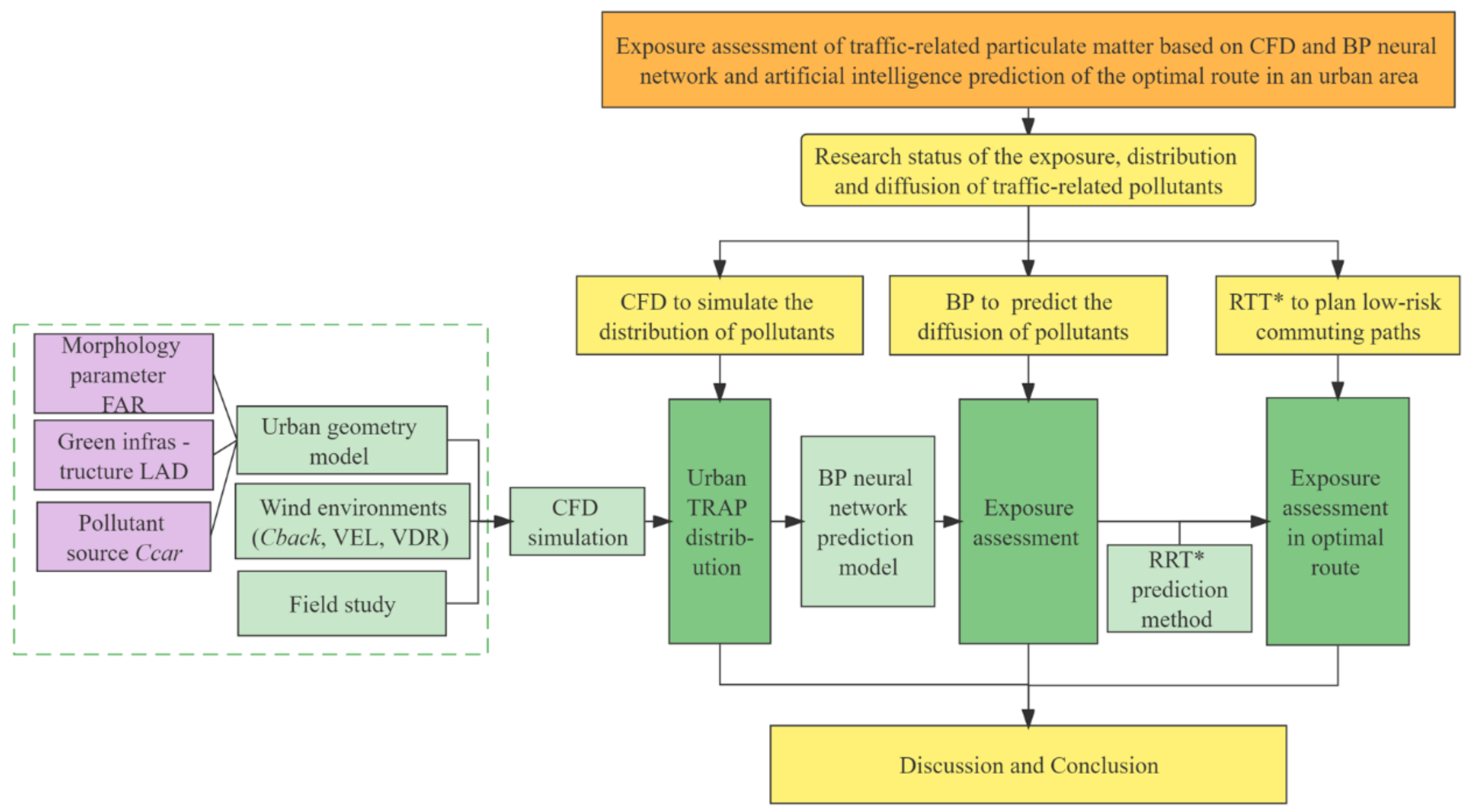
Exposure Assessment of Traffic-Related Air Pollution Based on CFD and BP Neural Network and Artificial Intelligence Prediction of Optimal Route in an Urban Area

Abstract

Due to rapid global economic development, the number of motor vehicles has increased sharply, causing significant traffic pollution and posing a threat to people’s health. People’s exposure to traffic-related particulate matter with an aerodynamic diameter less than 2.5 μm (PM_2.5) primarily occurs during commuting. Many studies have used exposure risk assessment models to assess the possible adverse effects of PM_2.5, but few have used them to plan low-risk pathways for commuters. This study simulated the pollutant concentration distribution in an idealized urban area in different scenarios. We then used a back propagation (BP) neural network to predict the pollutant concentration. The commuter respiratory deposition dose was calculated based on the BP prediction results, and the respiratory deposition dose was converted into obstacles on the commuting map. Finally, the rapidly exploring random tree star (RRT*) algorithm was used to plan low-risk paths for commuters. The results indicate that pollutants discharged by cars and tree planting can significantly affect the pollutant concentration. A 30.25 μg/m³ increase in the pollutant concentration discharged by cars resulted in a 7~13 μg/m³ increase in the traffic-related air pollution concentration on sidewalks. Combining a computational fluid dynamics simulation, a BP neural network model, and the RRT* algorithm provides a system to plan low-risk paths for commuters. This work proposes artificial-intelligence-based models for calculating the exposure risk to traffic-related pollutants (PM_2.5) and choosing a low-risk commuting path to ensure healthy travel.

1. Introduction

The global economy has developed rapidly in recent years, and the number of motor vehicles and the level of associated traffic-related air pollution (TRAP) have increased sharply. The negative impact of air pollution on human health has attracted wide attention, and motor vehicle exhaust emissions are the primary source of air pollution on urban roads. According to a report by the World Health Organization (WHO) in May 2018, approximately 4.2 million deaths a year are caused by exposure to polluted air [1].

Exposure to urban air pollutants leads to an increased risk of respiratory and cardiovascular diseases or premature death [2]. Fine particulate matter with an aerodynamic diameter of less than 2.5 μm (PM_2.5) is a critical environmental pollutant. It is associated with lung injury and several types of cancers [3], including oral, nasopharynx, esophagus, stomach, colorectal, liver, gallbladder, larynx, lung, bone, skin, female breast, cervix, prostate, and brain cancer and leukemia [4]. Children have significant vulnerabilities to PM exposure [5]. They have high respiratory pollutant intakes because of their higher ventilation rates and lung surface area versus weight ratio greater than adults [6]. Increased healthcare visits for childhood bronchitis during the cold season are significantly associated with the level of TRAP [7]. A one-year study of primary school children has shown that the levels of PM resulting from traffic exposure were associated with reductions in cognitive growth. Reducing air pollution from traffic near primary schools may improve cognition [8]. Traffic-related pollutants are associated with mortality, and although the risk is relatively low the public health impact of exposure to air pollution may be large because of the large number of exposed people [9].

Traffic pollution poses a serious threat to the health of commuters; thus, many scholars have carried out studies on traffic pollution and environmental epidemiology [10]. Many studies have focused on commuting and commuting methods because people’s exposure to pollutants is the highest during commuting.

An Italian study found that the cumulative exposure to ultrafine particles was 50% lower on the optimum commuting path than on the worst routes [11]. In one such study, people who took alternative routes substantially reduced the annual NO₂ concentrations to around 10 μg/m³, providing a method for children and their escorting parent to reduce the exposure risks to high NO₂ concentrations [12]. Some countries (Australia, New Zealand, Canada, UK) have proposed strategies [13,14] to influence children’s school travel behavior by focusing on education, motivation, encouragement, and infrastructure improvement to reduce children’s pollutant exposure during their commute [12].

The commuting mode also affects daily exposure risk. Active transportation modes such as walking are more physically demanding, increasing the ventilation rate and accelerating the exposure risk [15]. Gilliland et al. [16] tested the exposure to PM in 36 lower-grade students for different commuting types (walking, bus, and car). Those who walked to and from school had the lowest mean PM_2.5 exposure, whereas those that used buses or cars had higher exposures. On the other hand, when children’s commutes consisted of taking the bus and walking, the bus component resulted in a significantly higher mean personal exposure than the walking component. Tang et al. [17] tested people’s pollutant exposure for four major commuting transportation modes in Dublin, Ireland. The results showed that cyclists had the highest rates of PM_2.5 deposition in their lungs, followed by bus users, pedestrians, and automobile users. Car passengers had the highest absorption of volatile organic compounds (VOC_S), followed by cyclists, pedestrians, and bus users. Chaney et al. [18] found that active commuters received a greater PM_2.5 dose and had higher rates of exposure than other commuters.

High concentrations of TRAP are related to the pollutant source and the concentration distribution and diffusion of pollutants. Numerous investigations have been carried out in the last few decades to study the flow and pollutant dispersion in urban areas [19,20,21,22,23,24,25,26,27]. These can be categorized as three main research methods with distinct characteristics [28,29,30,31], including full-scale measurements, reduced-scale wind tunnel or water channel experiments, and numerical simulations using computational fluid dynamics (CFD). The first category provides measurements but is prone to uncontrollable factors and meteorological variability [32]. Although reduced-scale experiments can control boundary cases and building configurations, they must meet the similarity criteria and have high costs. CFD provides full control over the initial and boundary cases, as well as relevant parameter data for all points in the computing domain, combining the advantages of the other two methods. Cities are typically regarded as wind blockages in CFD simulations due to the city’s shape, building area density, and street configuration, according to Hang et al. [21]. The most important parameters affecting the air quality at the pedestrian level are the urban street width (WD) and street building height (BH) [33]. Pollutant dispersion is determined by urban airflow characteristics. The efficiency of removing pollutants by the wind depends on obstacles. Although tree plantings dilute pollutants, they also reduce the wind velocity (VEL) and affect the diffusion of pollutants [28].

In summary, the pollutant exposure of commuters depends on the commuting type, 3D building configuration, tree cover, and airflow characteristics. We propose a commuting path optimization to reduce the impact of traffic pollution on commuters. Recent research on pathway optimization has focused on transportation, logistics, numerical control, and cloud computing. However, few studies have applied pathway optimization to reduce pollutant exposure to commuters.

Many researchers have used neural network models to predict pollutant concentration, but these studies only forecast short- and mid-long-term concentrations of some well-known pollutants [34]. This study employs an artificial neural network (ANN) to predict the traffic-related PM_2.5 concentration, uses the predicted data to assess the exposure risk, and optimizes the commuting path using artificial intelligence to plan low-risk paths for commuters.

The flowchart of this study is shown in Figure 1. First, the research status of the exposure, distribution, and diffusion of traffic-related pollutants is presented. CFD is used to simulate the pollutant distribution for different cases using the building type, green infrastructure, and wind environment as variables. The resulting data are used to predict the pollutant concentration utilizing a back propagation (BP) neural network in an idealized urban area. The prediction results are converted into the respiratory deposition dose (RDD), representing the pollutant exposure on different roads to plan low-risk commuting paths using the rapidly exploring random tree star (RTT*) algorithm. The results provide urban designers with references for road network layout, green layout, wind environment, and other factors to improve urban air quality and create a sustainable city.

2. Methodology

2.1. CFD Simulation

2.1.1. Fundamental Theory

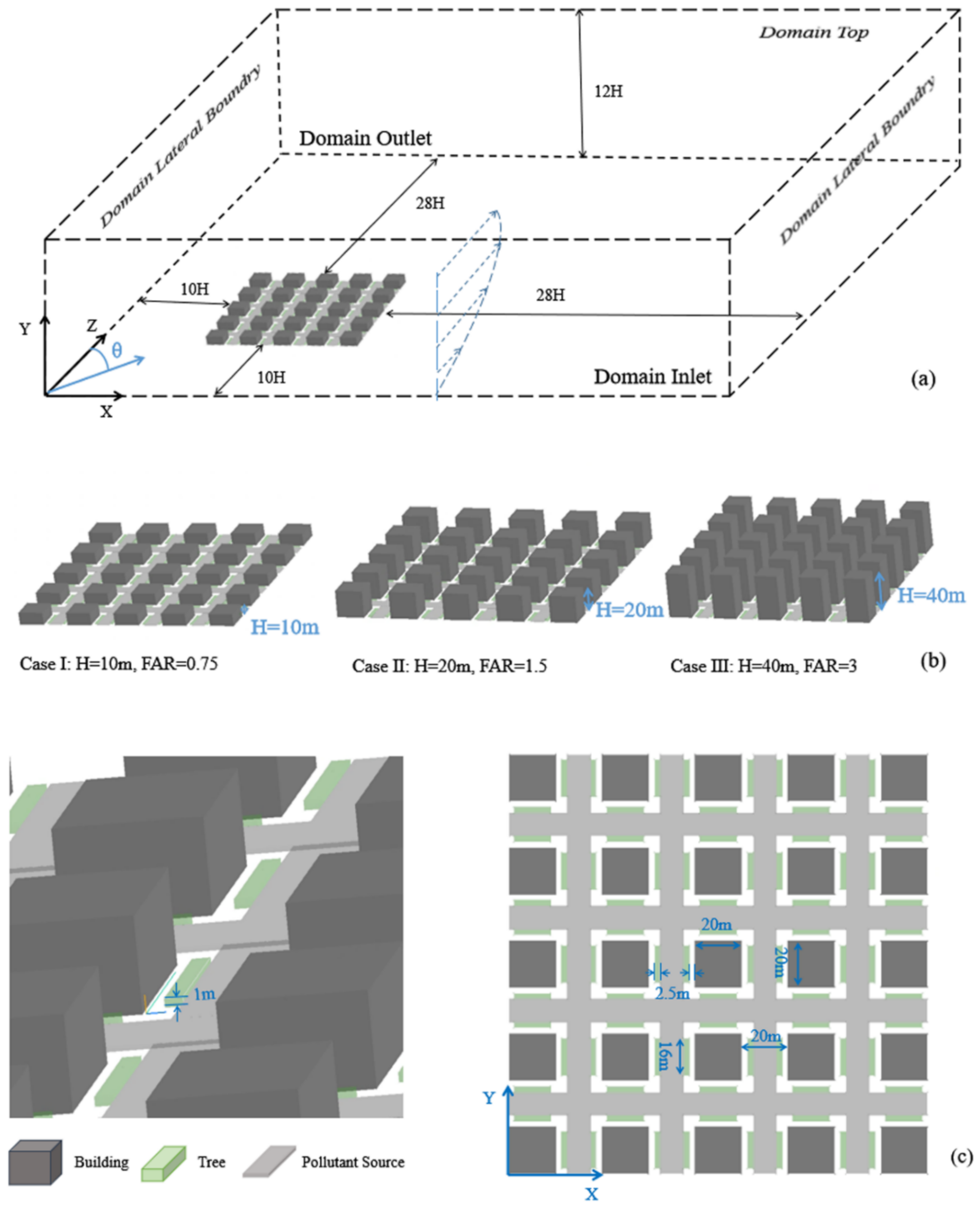
CFD simulations have been widely used for urban physics and computational wind engineering research in recent decades [35,36] and have been applied to a wide range of topics. Many studies have been summarized in several review articles [37,38,39]; therefore, we only provide an overview of this topic. CFD modeling with a high spatiotemporal resolution is an efficient and relatively low-cost method for studying flow and dispersion features. It provides control over the initial and boundary cases and whole flow field data, including outdoor and indoor air temperatures, water vapor concentration, CO₂ concentration, solar radiation, VEL, and wind direction. However, the accuracy and reliability of the CFD simulation are critical [40,41,42]. Therefore, solution verification and validation studies are particularly important. CFD turbulence simulations are often performed using Reynolds-averaged Navier–Stokes (RANS) approaches and large eddy simulations (LESs). LESs are more accurate than the RANS method for simulating and predicting turbulence [43,44,45]. However, the LES model requires substantial computational resources. Thus, RANS models are preferably used in turbulence simulations and have been successfully validated by wind tunnel measurements [46,47,48]. Despite the limitations, RANS simulations provide very good performance for general and more complex urban configurations [49,50,51,52]. In the RANS models, the standard k-ε model has excellent performance for predicting urban airflow and pollutant diffusion [53,54]. Thus, this study uses the PHOENICS 2021 software with the standard k-ε model for isotherm simulation using CFD.

The transport equations of the turbulent momentum (k) and its dissipation rate (ε) in the proposed CFD model are shown in Equations (1)–(7) [55]:

Continuity equation:

$$\frac{\partial {\overline{u}}_i}{\partial x_i}=0,$$

(1)

Momentum equation:

$${\overline{u}}_j\frac{\partial {\overline{u}}_i}{\partial x_i}=-\frac{1}{\rho }\frac{\partial \overline{P}}{\partial x_i}+\frac{\partial }{\partial x_j}\left(\nu \frac{\partial {\overline{u}}_i}{\partial x_j}-\overline{u_i^{\prime }{u}_j^{\prime }}\right),$$

(2)

$$-\overline{u_i^{\prime }{u}_j^{\prime }}={\nu }_t\left(\frac{\partial {\overline{u}}_i}{\partial x_j}+\frac{\partial {\overline{u}}_j}{\partial x_i}\right)-\frac{2}{3}k{\delta }_{ij},$$

(3)

k and ε equations:

$${\overline{u}}_i\frac{\partial k}{\partial x_i}=-\frac{\partial }{\partial x_i}\left[\left(\nu +\frac{\nu }{{\sigma }_k}\right)\frac{\partial k}{\partial x_i}\right]+\frac{1}{\rho }{P}_k-\epsilon ,$$

(4)

$${\overline{u}}_i\frac{\partial \epsilon }{\partial x_i}=\frac{\partial }{\partial x_i}\left[\left(\nu +\frac{{\nu }_t}{{\sigma }_{\epsilon }}\right)\frac{\partial \epsilon }{\partial x_i}\right]+\frac{1}{\rho }{C}_{\epsilon 1}\frac{\epsilon }{k}{P}_k-C_{\epsilon 2}\frac{{\epsilon }^2}{k},$$

(5)

$$v_t=\frac{C_{\mu }\cdot k^2}{\epsilon },$$

(6)

$$P_k=v_t·\left(\frac{\partial {\overline{u}}_i}{\partial x_j}+\frac{\partial {\overline{u}}_j}{\partial x_i}\right)·\frac{\partial {\overline{u}}_i}{\partial x_j},$$

(7)

where ${\overline{u}}_i$, ${\overline{u}}_j$, and $\overline{P}$ are the fluid velocity in the i direction, the fluid velocity in the direction, and fluid pressure, respectively; ρ is the fluid density; and δ_ij is the Kronecker delta. ν and ν_t are the kinematic viscosity and the kinematic turbulent viscosity; P_k is the volumetric production rate of k by shear forces; C_μ = 0.09.

The tree canopy on both sides of urban roads affects pollutant diffusion. The canopy and the individual branches are considered a porous medium in turbulence models [56]. The canopy produces drag and pressure, reducing the energy in the kinematic airflow and affecting atmospheric particle adsorption.

The flow resistance induced by turbulent flow through the plant canopy is described by the sink term in the momentum Equation (8) [57]:

$$S_{d,i}=-\rho \cdot C_d\cdot \alpha \left(z\right)\cdot {\overline{u}}_i\cdot \left|U\right|,$$

(8)

where C_d is the leaf drag coefficient, α(z) is the leaf area density (LAD) perpendicular to the flow direction in m²/m³, and $\left|U\right|$ is the magnitude of the superficial velocity vector.

The vegetation density is characterized by the LAD and its integral value, the leaf area index (LAI), which is defined by Equation (9):

$$\mathrm{LAI}={{\displaystyle \int }}_0^h\alpha \left(z\right)dz,$$

(9)

where h is the average height of the canopy in m. A vertically constant LAD is assumed for computational convenience. It is computed based on the LAI and canopy height (h) as:

$$\alpha =\frac{\mathrm{LAI}}{h},$$

(10)

The following additional source terms are added to the transport Equations (11) and (12) for k and ε to simulate the turbulent interaction between airflow and the plant canopy:

$$S_k=\rho C_d\alpha \left(z\right)\left({\beta }_p\cdot {\left|U\right|}^3-{\beta }_d\cdot \left|U\right|\cdot k\right),$$

(11)

$$S_{\epsilon }=\rho C_d\alpha \left(z\right)\left(C_{4\epsilon }{\beta }_p{\left|U\right|}^3\frac{\epsilon }{k}-C_{5\epsilon }{\beta }_d\left|U\right|\epsilon \right),$$

(12)

where S_κ and S_ε are the turbulent kinetic energy and turbulent dissipation rate of trees, respectively. Β_p, β_d, C_4Ɛ, and C_5Ɛ are empirical constants. The constant β_p is the portion of turbulent kinetic energy converted from the mean flow kinetic energy under the influence of drag, and β_d is the fraction of k dissipated by the short circuit of the energy cascade. The sink terms in these equations account for the spectral shortcut associated with the production of turbulence in the wakes behind the individual canopy elements, such as branches and leaves. The empirical constants must be adjusted to the measured data. The default values used in the PHOENICS implementation are those of Green [58], i.e., β_p = 1.0, β_d = 4.0, C_4Ɛ = 1.5, and C_5Ɛ = 1.5.

The modified generalized drift flux model takes into account the slip between the particle and the fluid phase [57]. In this model, the 3D tree model enhances the PM deposition through turbulent diffusion. The aerodynamic and deposition effects of plants on PM are represented by additional source and sink terms (S_sink and S_resuspension), enabling a comprehensive and accurate description and simulation of plant effects on PM dispersion [59]. The revised generalized drift flux model can be expressed as Equation (13):

$$\frac{\partial \left[(u_j+u_{slip})\cdot C\right]}{\partial x_j}=\frac{\partial }{\partial x_i}\left[{\epsilon }_p\frac{\partial C}{\partial x_j}\right]+S_c-S_{sink}+S_{resuspension},$$

(13)

However, the primary factor affecting particle slip include gravitational settlement, thermal force, and particle fluctuation. They are calculated as Equations (14)–(18) [57]:

$$u_{slip,j}={\tau }_p{g}_j+{\tau }_p\sum F_j+\frac{{\tau }_p}{C}{S}_{mj}-\frac{{\tau }_p}{C}\frac{\partial \left(u_{pj}{u}_{pi}C\right)}{\partial x_i},$$

(14)

$$S_{mj}=\frac{\partial }{\partial x_i}\left[{\epsilon }_{p}C\left(\frac{\partial u_{pj}}{\partial x_i}+\frac{\partial u_{pi}}{\partial x_j}\right)\right]+\left[\frac{\partial }{\partial x_i}{\epsilon }_p\left(u_{pi}\frac{\partial C}{\partial x_j}+u_{pj}\frac{\partial C}{\partial x_i}\right)\right],$$

(15)

$${\tau }_p=\frac{C_c{\rho }_p{d}_p^2}{18\mu },$$

(16)

$$S_{sink}=\mathrm{LAD}\times V_d\times C,$$

(17)

$$S_{resuspension}=S_{sink}\times \left(-0.00041v^2+0.017v-0.0016\right),$$

(18)

where u_slip,j is the gravitational settling velocity of particles in direction j (m/s). C is the particle concentration at the inlet (µg/m³). ε_p is the turbulent diffusivity (m²/s), which can be simplified to 1.0 m²/s [57,58]. S_c is the formation rate of the particle sources (kg/m³·s). S_sink is the mass of particles absorbed by the vegetation (µg/m³). S_resuspension is the secondary pollutant on the foliage (µg/m³·s) [60]. u_pj and u_pi are the particle velocities in the j and i directions (m/s), respectively. τ_p is the particle relaxation time (s). ΣF_j is the resultant force exerted upon the particle (m/s²). S_mj is the momentum source of the particle in the j direction kg/(m²·s²). µ is the molecular kinematic viscosity of air (Ns/m²). d_p is the particle diameter (m). C_c is the Cunningham factor induced by slippage. V_d is the particle deposition velocity on the foliage (m/s), and v is the magnitude of air velocity (m/s).

2.1.2. Urban Model

We simulated the flow field and pollutant diffusion on the street scale using CFD modeling. Three 3D idealized urban models were constructed. They were composed of a 5 × 5 building matrix with 25 cubes (L × L × BH = 20 m × 20 m × BH) representing the buildings with a plan area density (λ_p) of 0.25. The BHs of the three models are 10 m, 20 m, and 40 m, representing different floor area ratios (FARs). The WD is 20 m. Street trees (L₁ × L₂ × L₃ = 16 m × 2.5 m × 1 m) are located on both sides of the road. Figure 2a shows the simulation area of case I (BH = 10 m, FAR = 0.75) with a parallel approaching wind (θ = 180°) and dimensions of 580 m (X) × 580 m (Y) × 120 m (Z). The distance between the entrance (inflow boundary) and the target area is 10 BH, and the distance from the target area to the outlet (outlet boundary) is 28 BH. The distance between the left boundary and the target area is 10 BH, and the distance between the right boundary and the target area is 28 BH. The distance between the top and the ground boundary is 12 BH. The domain top has symmetric boundaries, while the domain outlet has a zero-gradient boundary [61].

The oncoming wind at the inlet has a gradient. The parameters are calculated by Equations (19)–(21):

$$U_{in}z=U_0\times {\left(\frac{z}{H}\right)}^{0.16},$$

(19)

$$k_{in}={(u^{*})}^2/\sqrt{C_{\mu }},$$

(20)

$${\epsilon }_{in}\left(z\right)=\frac{C_{in}^{\frac{3}{4}}{k}_{in}^{\frac{3}{2}}}{{\kappa }_{\nu }z},$$

(21)

where U₀ is the velocity at the height of 10 m and u* is the friction velocity. The von Kármán constant κ_v is 0.41. The empirical constant C_μ is 0.09.

2.1.3. Case Description

Three building configurations with heights of 10 m, 20 m, and 40 m representing different FARs were investigated to determine the influence of different FARs on the pollutant concentration of traffic-related PM. Five variables were selected to analyze the influence of green infrastructure, wind environment, and pollutant concentration discharged by cars on the pollutant distribution and diffusion: the background concentration (C_back), the VEL, the angle between the wind direction and true north (VDR), the LAD, and the concentration of pollutants discharged by cars (C_car). The details of three cases are summarized in

Table 1. Details of three cases in the numerical simulations.

FAR	Cback (μg/m3)	VEL (m/s)	VDR (θ + 180°)	LAD	Ccar (μg/m3)
I	12.10	1, 3, 5, 7	180°, 195°, 210°, 225°	0.25	90.75
	36.30	1, 3, 5, 7	180°, 195°, 210°, 225°	1.00	121.00
	60.50	1, 3, 5, 7	180°, 195°, 210°, 225°	4.00	151.25
II	12.10	1, 3, 5, 7	180°, 195°, 210°, 225°	0.25	90.75
	36.30	1, 3, 5, 7	180°, 195°, 210°, 225°	1.00	121.00
	60.50	1, 3, 5, 7	180°, 195°, 210°, 225°	4.00	151.25
III	12.10	1, 3, 5, 7	180°, 195°, 210°, 225°	0.25	90.75
	36.30	1, 3, 5, 7	180°, 195°, 210°, 225°	1.00	121.00
	60.50	1, 3, 5, 7	180°, 195°, 210°, 225°	4.00	151.25

. C_back and C_car are the PM contaminants (μg/m³).

2.1.4. Grid Description

A structural mesh was applied in this study, and a grid independence analysis was conducted. We chose 88 × 88 × 58 (coarse), 105 × 105 × 68 (medium), and 126 × 126 × 82 (fine) for the numbers of x, y, and z grids for case FAR II. We compared the TRAP concentration in the commuter breathing area at 1.6 m from the ground. The results are listed in

Table 2. Results of the grid independence analysis.

	Number of Cells in x, y, and z Directions	Relative Difference in the TRAP Concentration
Coarse grid	88 × 88 × 58
Medium grid	105 × 105 × 68	2.5%
Fine grid	126 × 126 × 82	1.1%

. As the computing unit increased from a coarse grid to a medium grid and fine grid, the relative differences in the pollutant concentrations were 2.5% and 1.1%, respectively. Thus, we chose the medium grid for the simulation. All the horizontal routes in the building area and the BHs were encrypted to ensure accurate results. There were about 740,000 cells, meeting the requirements recommended by the CFD Guide [62].

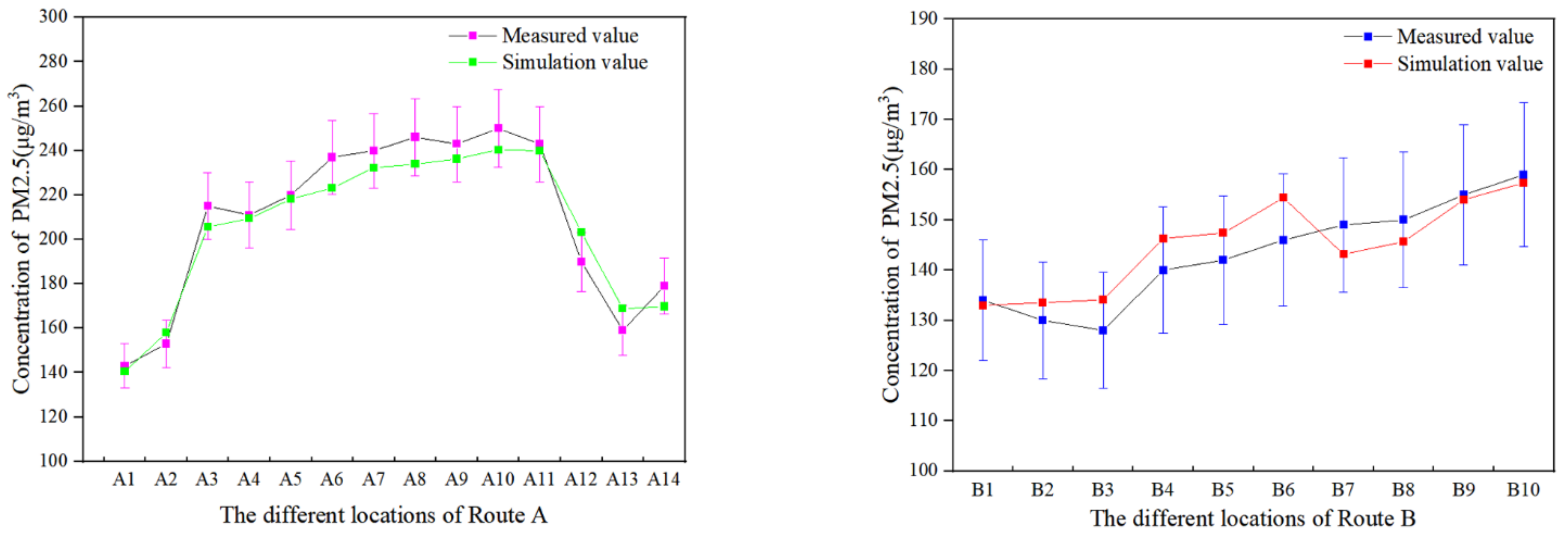
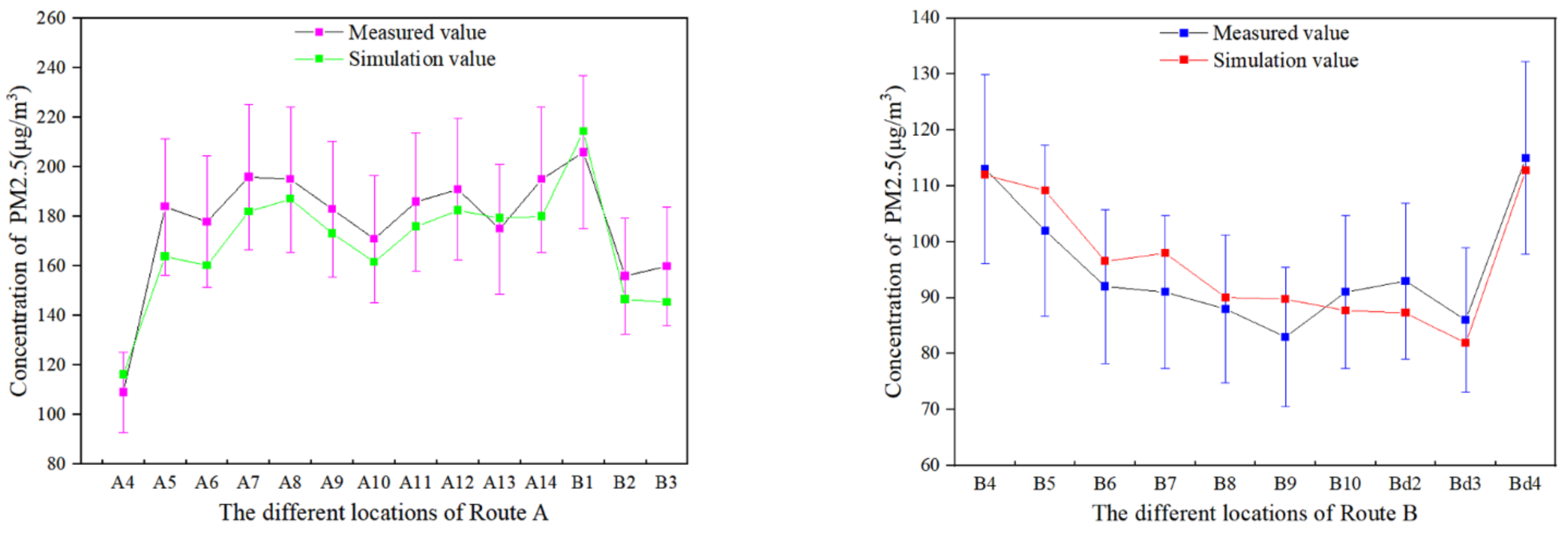
2.1.5. Simulation Validation

We measured the PM concentration on two different routes of a student commuter near a school in Jinan. The starting point of the test was the JianDa Garden Community, and the endpoint was the second school gate of Shandong Normal University. Route A consisted of busy main roads and intersections. The total length of route A was 760 m. Route B went through a residential area and park path. The total length of route B was 742 m, but it contained some steps. The key points of each route were numbered during the CFD simulations (Figure 3).

Two air quality detection instruments (CEMDT-9883M, China) were used to record the PM_2.5 and PM₁₀ concentrations on the routes. The instrument was placed in the tester’s backpack at a height of about 1.2 m, and the Global Positioning System (GPS) coordinates were recorded. The background PM concentration was obtained from the air quality monitoring point of Shandong Jianzhu University 1500 m from the study area.

We used Autodesk CAD to create maps of the buildings and roads and numbered each feature point. The data were exported as an STL file format and imported into PHOENICS. Two cases were used to validate the simulation accuracy. The parameters of case 1 were as follows: vehicle exhaust emission PM_2.5 concentration: 241.3 μg/m³; background PM_2.5 concentration: 92.9 μg/m³; VEL: 1 m/s; VDR: N. The parameters of case 2 were vehicle exhaust emission PM_2.5 concentration: 241.3 μg/m³; background PM_2.5 concentration: 65.1 μg/m³; VEL: 4.7 m/s; VDR: NW. These two cases were tested in January 2021, and the test period was 07:00–08:00. The weather on the test day was clear, and the average air temperature during the test was 3–5 °C. The results of the two validation cases are shown in Figure 4.

The measured and simulation values are shown in Figure 5 and Figure 6. The error is 7% for route A and 6% for route B for case 1 and 9% for case 2. Thus, the parameter values and boundaries of the PHOENICS simulation are accurate, and the results are credible.

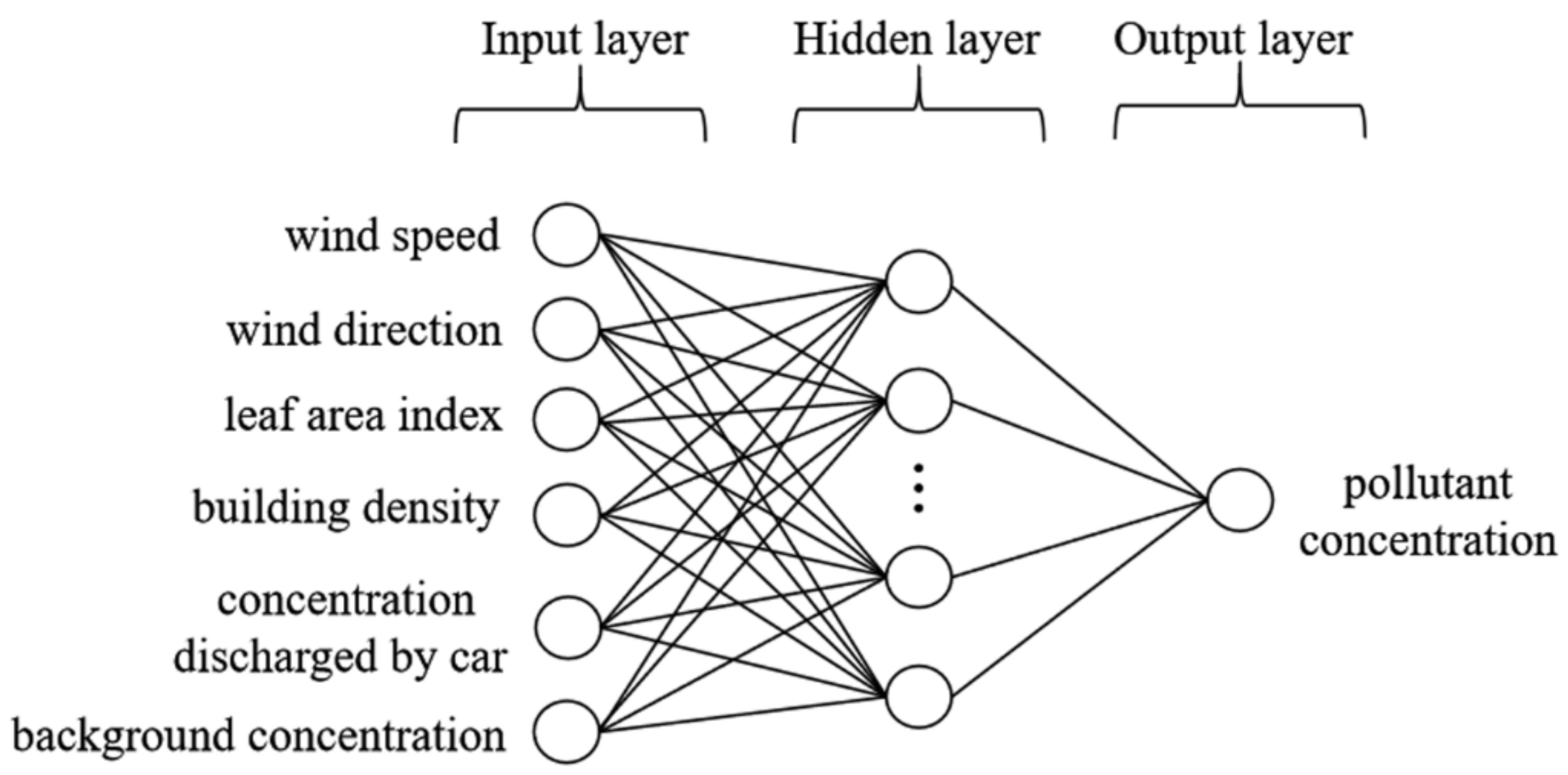
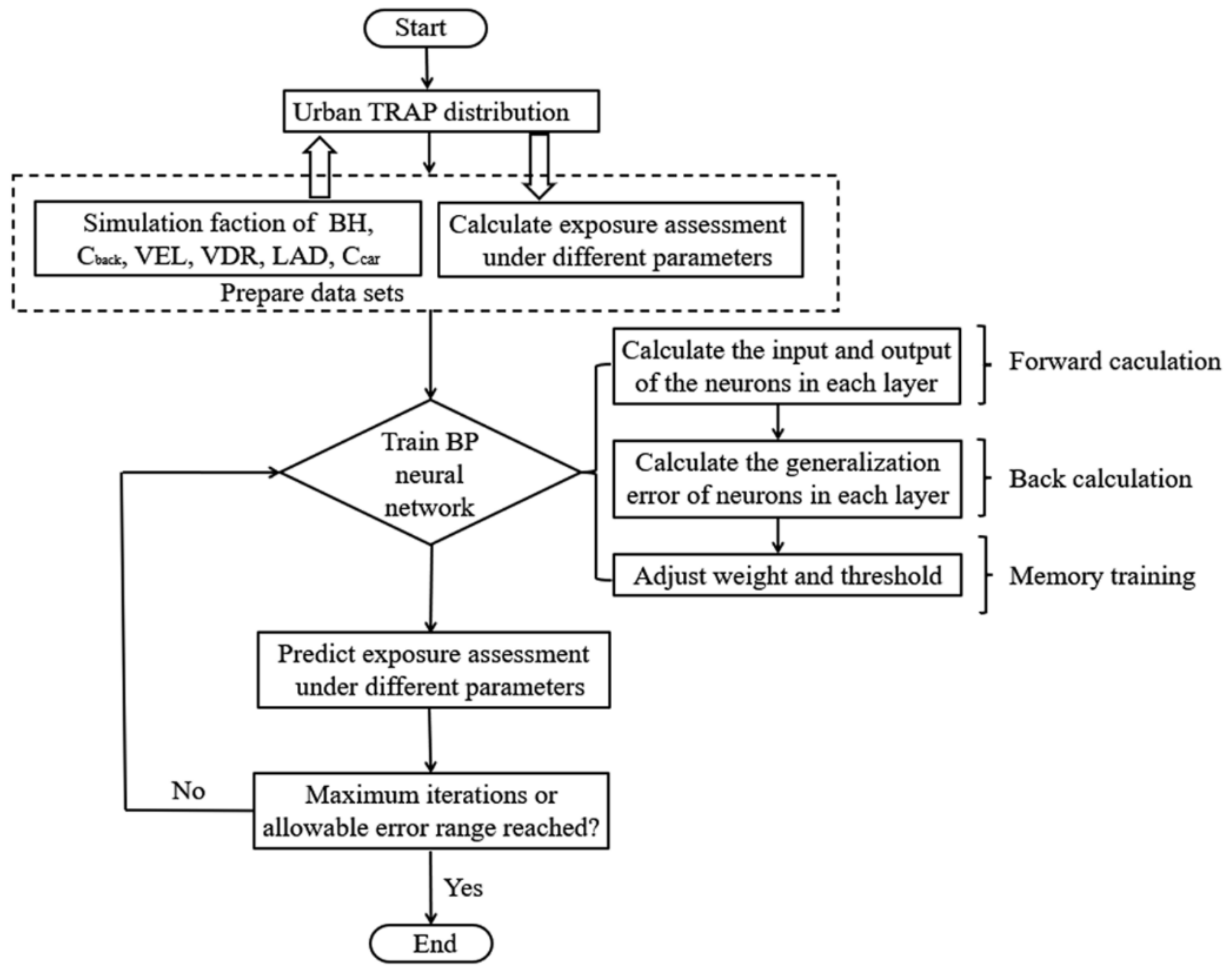
2.2. BP Neural Network

An ANN is a machine learning tool used to learn the relationship between input and output variables to predict system performance [63,64]. ANNs use many neurons in a topological structure to store and process complex information. An ANN includes an input layer, output layer, and one or more hidden layers. Each layer consists of neurons that receive signals from the previous layer and generate an output using an activation function. The most widely used ANN structure for prediction is the multi-layer perceptron (MLP) model. An MLP model with a single hidden layer with a sufficient number of neurons can approximate any function with the desired accuracy [65]. The MLP network consists of the input, hidden, and output layers; all inputs are connected to the neurons, and all neurons are connected to the output. Therefore, this study established an MLP network to predict the effect of the variables on pollutant diffusion.

In an MLP network, the correlation between the input x(k) and output y(k) is expressed as Equations (22) and (23) [66]:

$$y\left(k\right)=f_2\left(w^{2}x\left(k\right)+b_2\right),$$

(22)

$$x\left(k\right)=f_1\left(w^{1}x\left(k\right)+b_1\right),$$

(23)

where x(k) is the output vector from the hidden layer. w¹ and w² represent the connection weight matrices from the input layer to the hidden layer and from the hidden layer to the output layer, respectively. f₁(.) and f₂(.) represent the transfer functions of the hidden and output layers, respectively, and b₁ and b₂ represent the numbers of deviations in the input and output layers, respectively. The transfer function used in this study is a tangent s-type function, which is defined in Equation (24) [67]:

$$f\left(z\right)=\frac{\left(1-e^{-2z}\right)}{\left(1+e^{-2z}\right)},$$

(24)

where z represents z = f(Σw_ix_i), where x_i is the input of the neuron, w_i is the weighting factor of the input, and z is the weighted input. We used the root mean square error (RMSE) to measure the prediction accuracy; it is defined by Equation (25) [68]:

$$RMSE=\sqrt{\frac{1}{p}{{\displaystyle \sum }}_j{\left|t_j-o_j\right|}^2},$$

(25)

where p is the number of measurements, t_j is the target value, and o_j is the output value.

The training procedure was performed by optimizing the weights and bias coefficients to minimize the error between the target and the neural network output. A BP neural network was used in this study. The structure of the ANN is shown in Figure 7; it has 6 inputs, 10 neurons, and 1 output. The input values are the C_back, VEL, VDR, LAD, FAR, and C_car. The output values were classified into different exposure levels. The 1296 outputs obtained from the simulation were divided into two parts; 70% of the data was randomly selected for neural network training, and the remaining 30% was used for validation.

The BP neural network model is a multi-layer feed-forward neural network that submits samples to the network according to a preset error. When the network converges, the training ends. When the number of training iterations reaches the maximum value, the training is terminated, representing the end of the learning process if the network does not converge. Error propagation is performed by continuous training based on error feedback until the case requirements are met or the network is trained to the maximum number of iterations [69]. BP neural networks are mainly used for function approximation, relationship recognition, data classification, and data compression. When a BP neural network is used as the core of a predictive model, it functions approximately as a nonlinear model.

Figure 8 shows the flowchart of the BP neural network algorithm. The computational process of the BP neural network consists of forward and backward propagation. In the forward propagation, the input signal from the input layer is processed by each layer and transmitted to the output layer. The state of neurons in each layer affects only the state of neurons in the next layer. The output layer compares the actual output value with the expected output value. If the output layer does not obtain the desired output, the error is back propagated along the original connection path, and the error is minimized by modifying the weights of each neuron. The training and learning of the BP neural network model consist of taking the error signal as the basis for modifying neuronal weight and performing forward and back propagation to obtain the expected accuracy or the predetermined maximum number of training epochs.

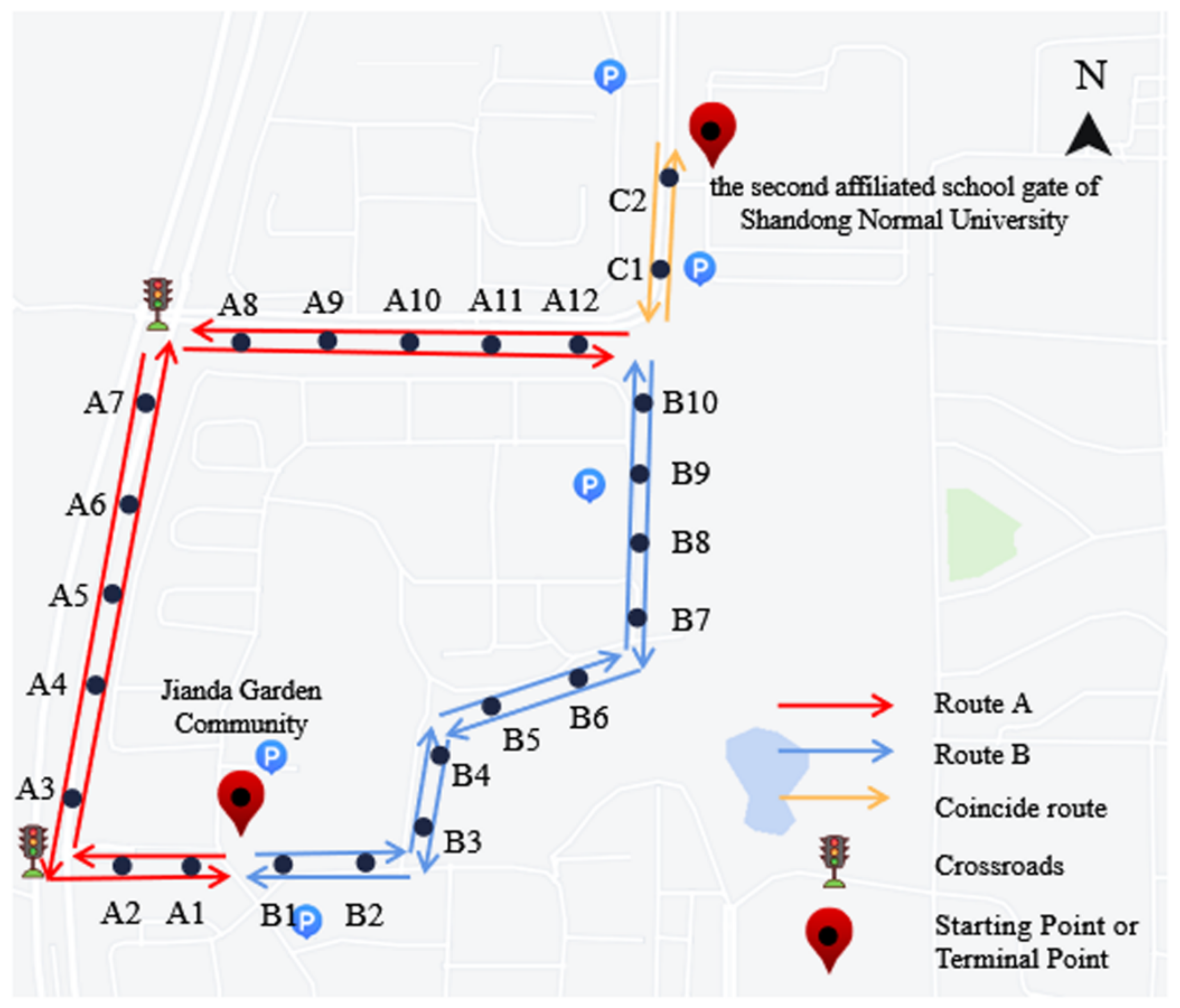
2.3. Optimal Path Prediction

2.3.1. RRT* Algorithm

The rapidly exploring random tree algorithm (RRT) algorithm is a path planning algorithm based on random sampling. It was proposed by LaValle et al. in a complex environment. The RRT algorithm does not require a function expression of the planning space. It uses sampling point collision detection to avoid obstacles and plan the optimal path between nodes. Therefore, it can solve high-dimensional path planning problems with complex constraints and has the advantages of probabilistic completeness and strong scalability. However, since it uses machine learning for searching, the convergence speed is relatively slow, and the generated path is not necessarily the optimal path. To optimize the RRT algorithm, scholars have thus proposed the RRT* algorithm, which reconnects the trees, finds new low-cost paths in the tree nodes, reduces the path length, and converges to the optimal solution. The RRT* algorithm constructs a path by randomly selecting points in the search space.

The search space is constructed first with an empty tree, and the starting point is added to the tree as the root node. When the algorithm is executed, the starting point is the initial point (X_initial). A random point (X_random) is created according to the random function. The Euclidean distance is used to find the nearest point X_nearest on the tree to connect X_random to X_nearest. X_random becomes the center with r_i as the radius. The algorithm searches for nodes on the tree to identify a potential set of parent nodes X_{potential_parent}. It then calculates the cost of X_parent as parent 1 and selects a potential parent node X_{potential_parent}. If no collision occurs, the algorithm connects X_{potential_parent} to X_random, calculates the cost of path 2, and compares cost 2 to cost 1. Collision detection is performed if cost 2 is smaller than cost 1. Otherwise, the algorithm selects the next potential parent node. If the collision detection fails, the potential parent cannot act as the new parent, and the next potential parent node is considered. The above steps are repeated. If a collision is detected, the algorithm deletes the previous edges in the tree and adds new edges using X_{potential_parent} as X_parent. It then traverses through all the potential parents to obtain an updated tree. These steps are repeated to complete route planning.

2.3.2. Exposure Evaluation Indices

TRAP exposure assessments have considered external and internal exposures. Studies on the spatiotemporal distribution of traffic-related particles have mostly used external exposure evaluations. The RDD is commonly used to assess pollutant exposure levels in China. It is calculated using Equation (26):

$$RD{D}_{PMfractions, i}=\left(VT\times f\right)\times D{F}_i\times P{M}_i,$$

(26)

The RDD_{PM(fractions,i)} is the respiratory deposition dose of the measured pollutant (μg/s), and DF_i and PM_i (μg/m³) are the deposition rate and concentration of the group i particles, respectively. In addition, the median mass diameters (d_p, μm) of different-sized PMs are calculated using Equations (27) and (28):

$$DF=IF(0.0587+\frac{0.911}{1+\mathit{exp}(4.77+1.485ln d_p)}+\frac{0.943}{1+\mathit{exp}(0.508-2.58ln d_p)}),$$

(27)

$$IF=1-0.51(1-\frac{1}{1+0.00076{d_p}^{2.8}}),$$

(28)

where IF is the inhalable fraction and d_p (μg) is the mean particle diameter of the coarse and fine-grained fractions. VT is the tidal volume, and the f is the typical respiratory rate. The values of VT = 1250 cm³ and f = 0.34 times/s are chosen according to the reference by Hinds [70].

2.3.3. The RRT* Path Planning Algorithm

First, we predicted the pollutant concentration using the BP to calculate the RDD_PMi. The results were ranked from small to large. We determined the radius range of the newly added obstacle areas R₁~Rn according to the road width in the designated area, where R₁ = 0, R_n is half of the widest road width, and n is the number of calculated RDDs. The radius of the newly added obstacle area could not exceed R_n to prevent the excess area covered by the barrier area from affecting the commuting path planning. The RDD values were standardized and ranked from small to large, where RDD_PMi corresponded to R_i (Figure 9). The center of each obstacle area was located at the road center and contained the building layout, transportation network, and the calculated PM_2.5 exposure risk. The map was imported into the RRT* algorithm to determine the optimal commuting path. The results are shown in Section 3.3.

3. Results

3.1. CFD Simulation Results

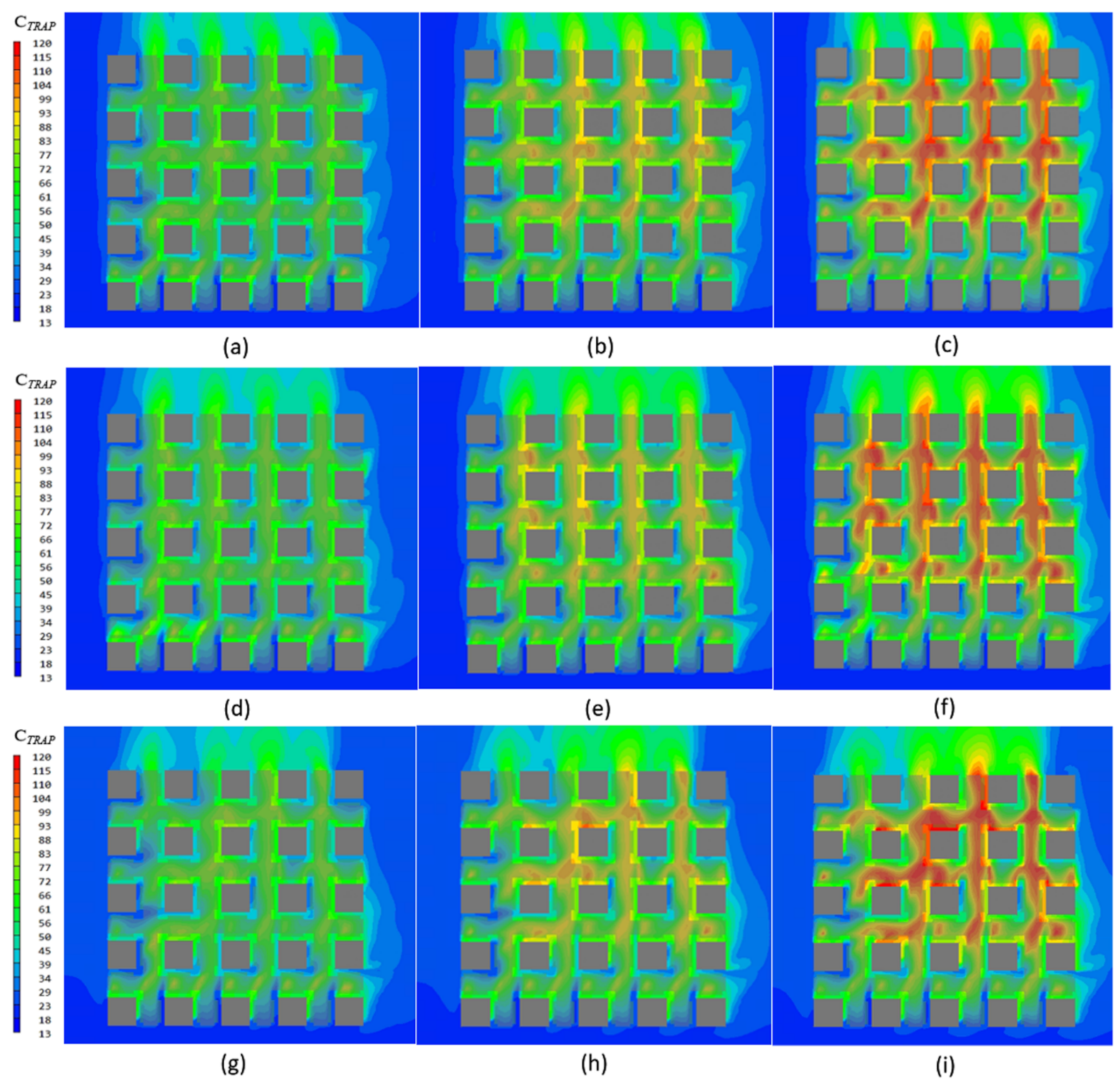
3.1.1. Impacts of Pollutant Concentration Discharged by Cars on the Pollutant Distribution and Diffusion

After the CFD simulation, we selected 15 points on each road around the center buildings to determine the pollutant concentration using Python (Figure 10). We averaged the values of 60 points to represent the pollutant concentration in this area. It was found that the concentration of traffic-related fine particles increased with an increase in the traffic flow for different values of the BH, C_back, VEL, VDR, and LAD. The TRAP concentrations (C_TRAP) on sidewalks increased by about 7–13 μg/m³ for each 30.25 μg/m³ increase in C_car. The dilution level of the pollutants by the wind differed for different C_car values. When C_car was 90.75 μg/m³, C_TRAP decreased by about 2.8% for every 2 m/s increase in VEL. When C_car was 121.00 μg/m³, C_TRAP decreased by about 3.5% for every 2 m/s increase in VEL. When C_car was 151.25 μg/m³, C_TRAP decreased by about 4.0% for every 2 m/s increase in VEL. The results for a BH of 20 m, C_back = 12.10 μg/m³, VDR = 195°, and LAD = 0.25 are shown in Figure 11.

We assessed adult male commuters. Since the breathing area of adult men is located at the height of 1.5–1.6 m, we used a height of 1.6 m in the CFD simulation to evaluate the pollutant exposure of commuters. A comparison of Figure 11a–c shows that the pollutant concentration in this ideal urban block increased with the pollutant concentration released by vehicles. The same pattern is observed when the wind speed increased to 5 m/s and 7 m/s (Figure 11d–i). In addition, the buildings represent obstacles to the wind. Therefore, commuters should avoid longer traffic paths to reduce the exposure risk.

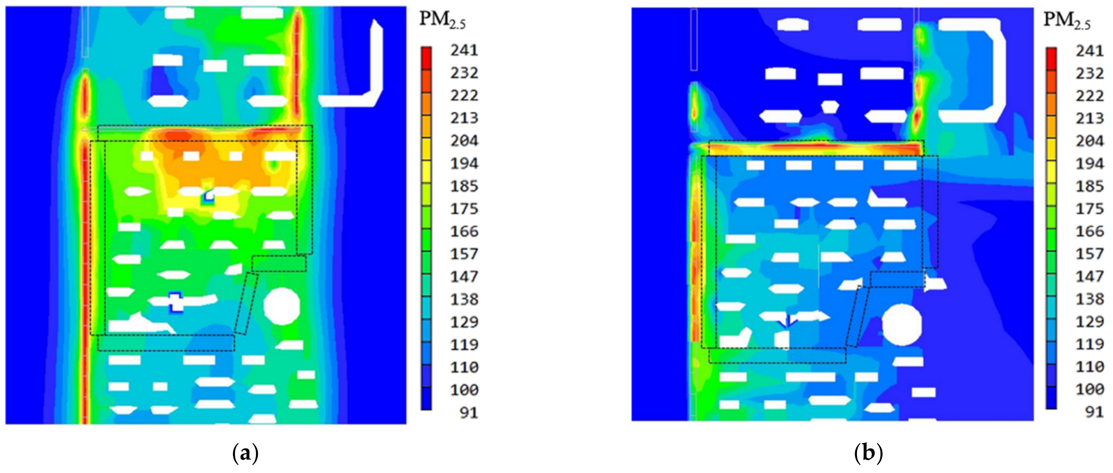
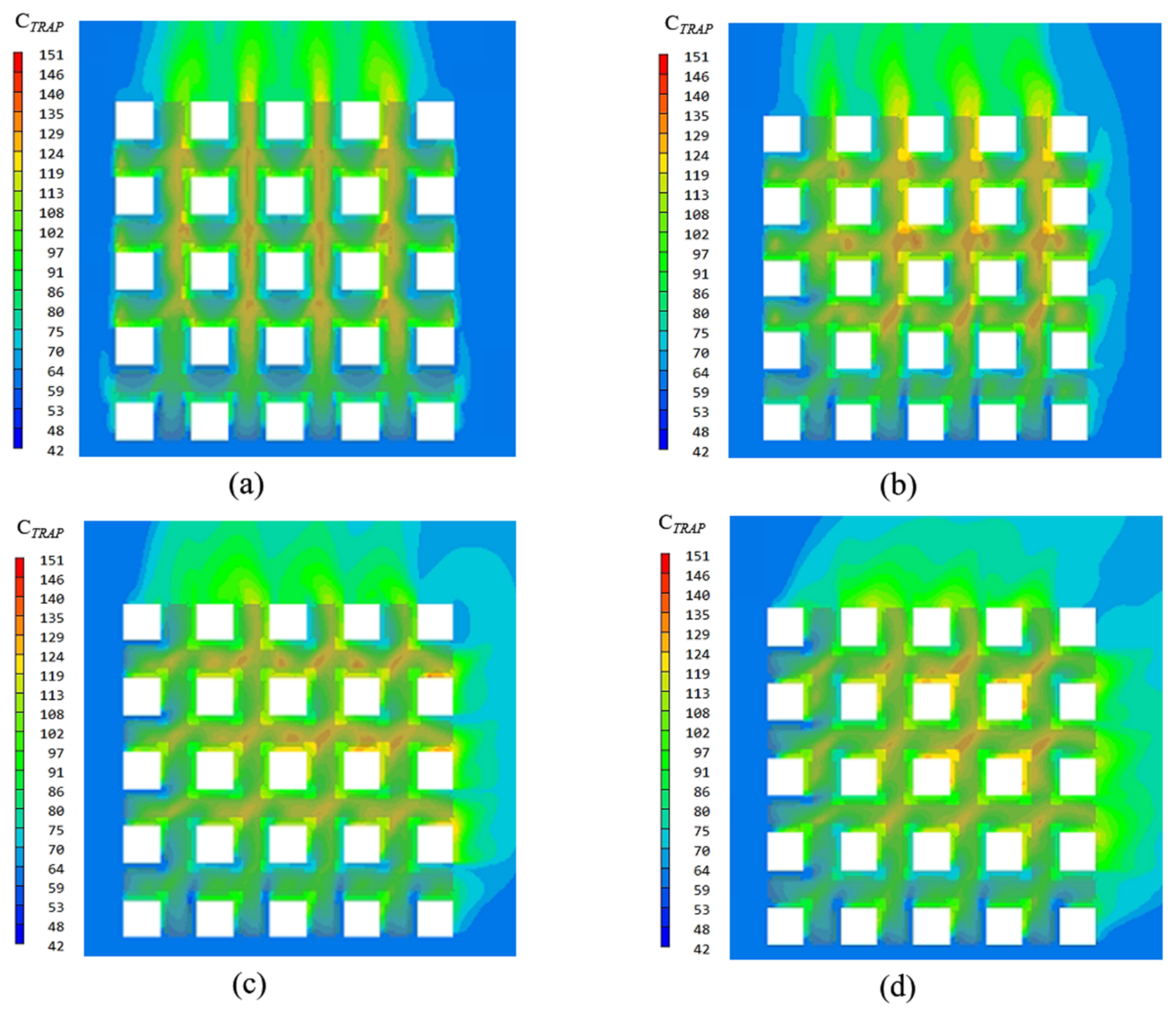
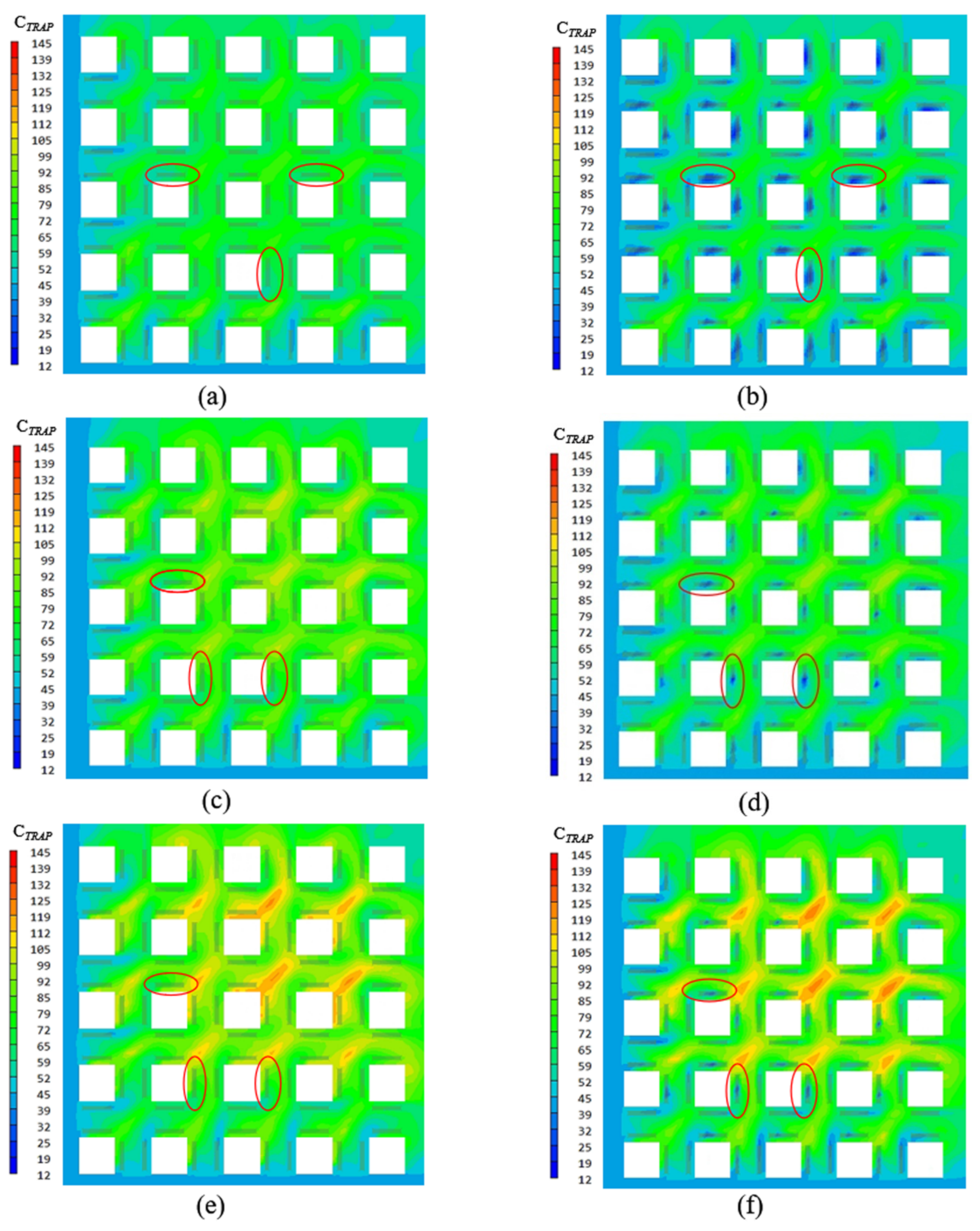
3.1.2. Impacts of Wind Direction on the Pollutant Distribution and Diffusion

The diffusion of traffic-related particles is related to the VDR. The influence of different VDRs on the TRAP distribution was evaluated for a BH of 20 m, C_back = 60.50 μg/m³, C_car = 151.25 μg/m³, VEL = 3.0 m/s, and LAD = 1.00. The simulation results for different VDRs are shown in Figure 12. The distribution of the traffic-related pollutants differs for different VDRs, leading to large differences in the distribution of particulate matter on different routes. The pollutants are more likely to be diffused when the street direction is parallel to the wind direction. In contrast, pollutants accumulate in streets perpendicular to the wind direction. In addition, the pollutant accumulation differs for different wind directions. However, most of the pollutants accumulate at the junction of the downwind area of the building. Therefore, the influence of wind speed should be considered when planning low-risk paths.

3.1.3. Impacts of Trees on the Distribution and Diffusion of Pollutants

Figure 13 shows the influence of three different tree configurations on the pollutant distribution for a BH of 20 m, VEL of 3.0 m/s, and VDR of 225°. Figure 13b,d,f show the results for an LAD of 4.0, and Figure 13a,c,e show the results for an LAD of 1.0. The pollutant concentration was significantly lower in areas with trees on both sides of the road than in other areas, indicating that trees dilute the pollutant concentration. At a Ccar of 90.75 μg/m³, the C_TRAP in the two building blocks was 60–80 μg/m³ with LADs of 1.0 and 4.0. However, for an LAD of 4.0, the C_TRAP was 12 μg/m³ in areas with trees on both sides of the road. As the C_car increased, the pollutant concentration increased for LADs of 1.0 and 4.0, but it decreased in areas with trees on both sides of the road for an LAD of 4.0. Therefore, commuters should choose routes with a large LAD such as parks to avoid exposure to high pollutant concentrations.

3.1.4. Impacts of Background Concentration on the Pollutant Distribution

Figure 14a–c show the pollutant concentrations at C_back values of 12.10, 36.30, and 60.50 μg/m³, respectively. The CFD simulation results show an increase in the pollutant concentration within the regular building space with the background concentration. Although the wind direction is parallel to the street direction, the pollutants accumulate with an increase in the background concentration. At a C_back of 12.10 μg/m³, the pollutant concentration was significantly higher inside than outside of the block, but the accumulation of pollutants was not obvious. At a C_back of 36.30 μg/m³, the pollutant concentration increased inside and outside of the block. When C_back reached 60.50 μg/m³, the pollutant concentration increased again. When the C_back was 36.30 μg/m³ and 60.50 μg/m³, the pollutant concentration was very high and most pollutants had accumulated at the intersection of the downwind building space exit and the downwind area. Therefore, a change in C_back affects the choice of the commuting path by affecting the pollutant distribution. The high-concentration areas should be avoided.

3.2. BP Neural Network Prediction

3.2.1. Training Result of BP Neural Network

The BP neural network was implemented in Python, and the data obtained from the CFD simulation were used to train the model. The concentration of traffic-related pollutants in the normal configuration was predicted for different cases. Figure 15 shows the training results of the BP neural network for predicting the pollutant concentration. The results are consistent with the simulation results. The coefficient of determination (R²) for the predicted and simulated pollutant concentrations was 0.9459, and the RMSE value was 0.4327. The high R² value indicates a good fit for the BP neural network.

3.2.2. Validation Result of BP Neural Network

A well-trained model was obtained by the repeated training and continuous debugging of the learning rate of the BP neural network. The validation results are shown in Figure 16. The R² and RMSE of the predicted and simulated pollutant concentrations were 0.9072 and 0.3339, respectively, indicating a good fit for the BP neural network.

3.2.3. Prediction Results of BP Neural Network

The results show that the proposed BP neural network model provides accurate predictions of traffic-related PM concentrations. Commuting routes with a lower exposure can be selected based on the predicted pollutant concentrations. We used the BH, C_back, VEL, VDR, LAD, and traffic flow as input variables and predicted the pollutant concentration for different cases to perform path optimization. The results show that the pollutant concentration increased with the BH (Figure 17).

3.3. Optimal Routes Obtained from the RRT* Algorithm

3.3.1. Exposure Analysis

We calculated the RDD values according to the BP prediction results to assess the pollutant exposure risk of commuters for different cases.

Table 3. Exposure analysis results for different C_car and VDR values.

FAR	Cback (μg/m3)	VEL (m/s)	VDR	LAD	Ccar (μg/m3)	CTRAP (μg/m3)	RDD (μg/min)
I	60.50	1	225°	4.00	36.30	25.30	0.60
	60.50	1	225°	4.00	60.50	24.30	0.58
	60.50	1	225°	4.00	90.75	28.18	0.67
	60.50	1	225°	4.00	121.00	34.92	0.83
	60.50	1	225°	4.00	151.25	30.97	0.74
	60.50	1	195°	4.00	36.30	40.89	0.97
	60.50	1	195°	4.00	60.50	38.81	0.92
	60.50	1	195°	4.00	90.75	47.05	1.12
	60.50	1	195°	4.00	121.00	51.77	1.23
	60.50	1	195°	4.00	151.25	49.13	1.17
	60.50	1	180°	4.00	36.30	37.31	0.89
	60.50	1	180°	4.00	60.50	40.81	0.97
	60.50	1	180°	4.00	90.75	43.14	1.03
	60.50	1	180°	4.00	121.00	46.60	1.11
	60.50	1	180°	4.00	151.25	53.35	1.27

lists the C_TRAP and RDD values for C_car values of 36.30, 60.50, 90.75, 121.00, and 151.25 μg/m³ and VDRs of 225°, 195°, and 180° at FAR I, VEL = 1 m/s, and LAD = 4. The RDD value was calculated for adult men walking on the street. The VDR was 225°, the C_car was 36.30 μg/m³, and the RDD value was 0.60 μg/min. As the concentration of pollutants released by vehicles increased, the RDD value showed an upward trend. The maximum RDD value (0.83 μg/min) occurred at a C_car of 121 μg/m³. As the C_car increased to 151.25 μg/m³, the RDD decreased to 0.74 μg/min. The values of the RDD differed for different wind directions. These results are in agreement with the CFD simulations.

3.3.2. Optimal Routes

We constructed an idealized building space with a height of 10 m, a background concentration of 0.005, and an LAD of 4.00 to assess the influence of different VDRs, VELs, and C_car values on the choice of commuting path. The wind directions were 180°, 195°, and 225°, and the wind speed was 1.0 m/s. The C_car ranged from 36.30 μg/m³ to 151.25 μg/m³. The results of the BP prediction for different cases were converted to the exposure assessment value, and obstacles were drawn on the map according to the exposure level. The distance and exposure risk were considered, and two routes with the shortest distance and lowest exposure risk were obtained.

The commuting maps are shown in Figure 18a,c,e. The optimal path obtained from the RRT* algorithm is shown in Figure 18b,d,f. The exposure risk ranges in the configuration space were 1.22–1.75 μg/min, 1.34–1.61 μg/min, and 0.83–1.02 μg/min for VDRs of 180°, 195°, and 225°, respectively, and the corresponding R1~Rn was 1~10 m. As the VDR increased, the RDD of the C_TRAP on the road increased and the exposure risk decreased.

The exposure risk represented by the circular radius can only be compared for the same working condition. The results show that the RRT* algorithm can plan the optimum target route for the three working conditions. When the range of exposure risk is large, the route includes more turns, and when it is small, there are more straight-line sections. When the exposure risk has a large range, so does the radius of the circular obstacles, and more roads can be selected. Therefore, using the algorithm for optimal path selection is advantageous when the pollutant concentration is variable.

4. Discussion

Three-dimensional idealized city models consisting of 5 × 5 building matrices were constructed, and the effects of the building type, green infrastructure, and wind environment on the pollutant distribution and concentration were evaluated. CFD was used to simulate the pollutant distribution of 1296 cases for three heights. The CFD simulation results were used as input into a BP neural network model. A good fit of the model was obtained for predicting the pollutant concentration for different cases. The BP prediction results were converted into the RDD to represent the pollutant exposure on different commuting paths. Path optimization was performed using the RTT* algorithm.

It should be noted that nitrogen oxides, VOCs, and inert gases, such as CO, are traffic-related air pollutants. However, we did not analyze them because this paper focuses on the impact of particulate matter on commuters.

This study focuses on the prediction and distribution of pollutants and path assessment under the idealized urban area and does not carry out relevant research on the actual urban area, which is the deficiency of this study. In fact, there have been a lot of relevant studies which have done a lot of work on actual, specific building distributions. Taking a large city in Poland as an example, Kwiecień et al. [71] proposed a comprehensive research method to evaluate CO concentration in road traffic. Hang et al. [20] studied the impact of building height on pollutants, and Gu et al. [72] studied the impact of building density on pollutants. Hang et al. also studied the distribution of pollutants under different aspect ratios. However, in order to obtain some regular conclusions more intuitively and obviously, such as the changes in pollutant concentration with different wind speed changes, this paper only considers the regular and ideal types. In the future, a lot of research could be carried out on actual buildings. The wind environment significantly influences pollutant distribution and diffusion. Previous studies have shown that increasing urban airflow can dilute pollutants [73,74]. However, in our CFD simulation, the pollutant concentration increased with an increase in the velocity in local areas. Studies have shown that urban tree planting can weaken pollutant dilution. However, we did not observe that the vegetation reduced the wind speed in this simulation. Due to uncontrollable factors, such as closure and control during the COVID-19 pandemic, the simulation was only validated using limited cases. More scenes should be used for the validation to ensure that the simulation result is credible. This paper only assessed the pollutant exposure of adult male pedestrians for path planning. However, the pollutant exposure during commuting depends on the person, commuting mode, and commuting time [75]. Active commuters received a higher PM_2.5 dose and had higher rates of exposure than other commuters [18]. Kumar et al. [76] measured the particle number concentration (PNC), PM₁, and PM_2.5 concentrations along an established route covering bus stops, primary schools, universities, and intersections. The PM_2.5 and PM₁ concentrations and the PNC in the morning were 47%, 31%, and 31% higher, respectively, than those in the afternoon, and the concentration of coarse particles was 70% higher in the afternoon. Garcia-Algar [77] found that the pollutant concentration is higher at the height of a stroller than in the respiratory area of adults. An et al. [75] and Ahmed et al. [12] observed that the exposure of commuters to pollutants depends on the commuter route. Therefore, future studies should consider the commuting time and mode and the unequal exposure of people for path planning.

5. Conclusions

This study simulated the pollutant concentration and distribution for different urban morphological parameters and green infrastructure scenarios. We converted the simulated pollutant concentration into the respiratory deposition to assess the exposure risk. The traffic-related fine PM exposure risk was mapped to perform path planning using the RRT* algorithm in an idealized urban area, which provided the shortest commuting distance and the lowest exposure risk. The novelty of this paper is the combination of a CFD simulation, BP neural network model, and RRT* algorithm to create a system to plan low-risk paths for commuters. The results provide urban designers with references for road network layout, green layout, wind environment, and other factors to improve urban air quality and create a sustainable city. The following conclusions were obtained:

(1)

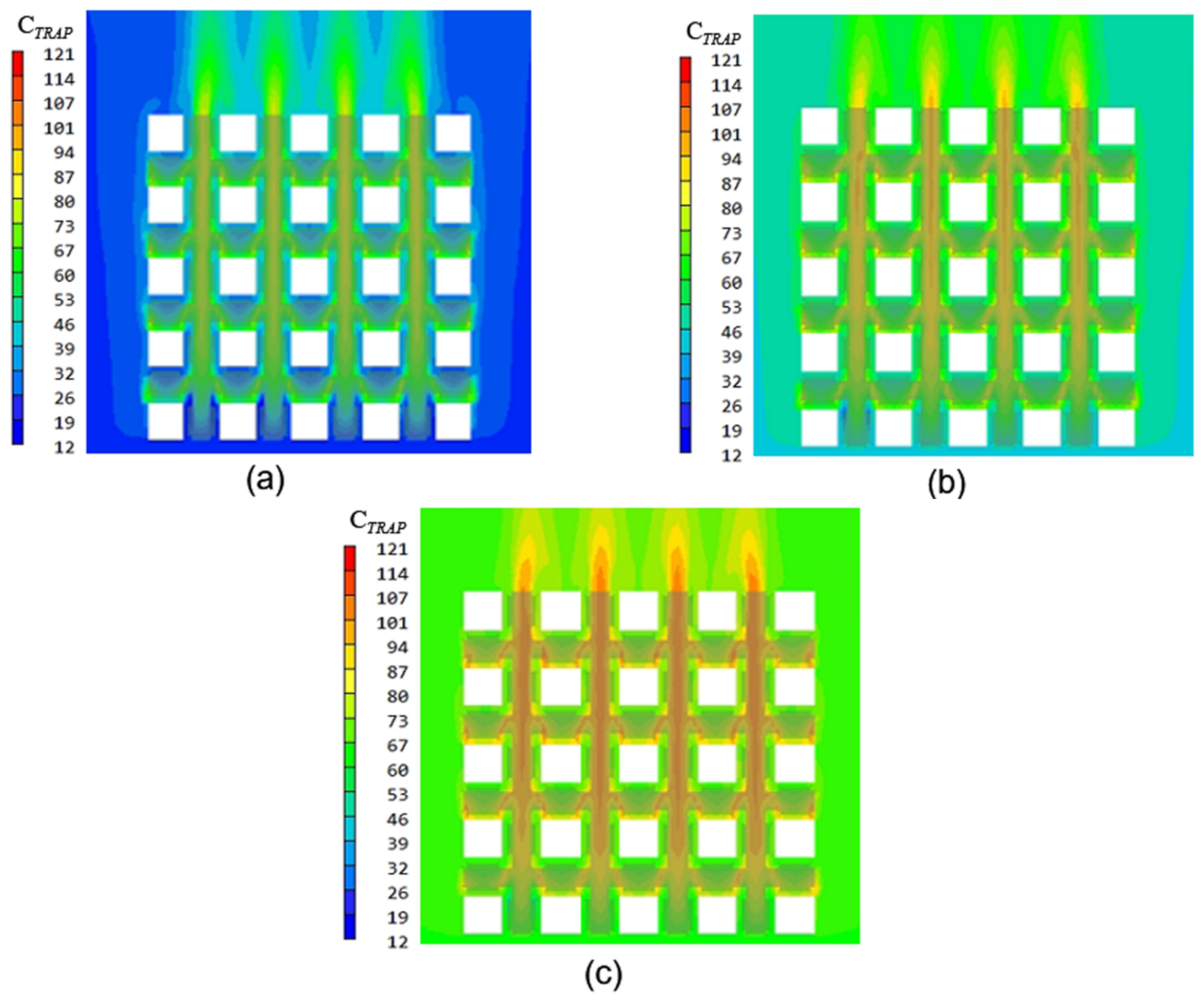
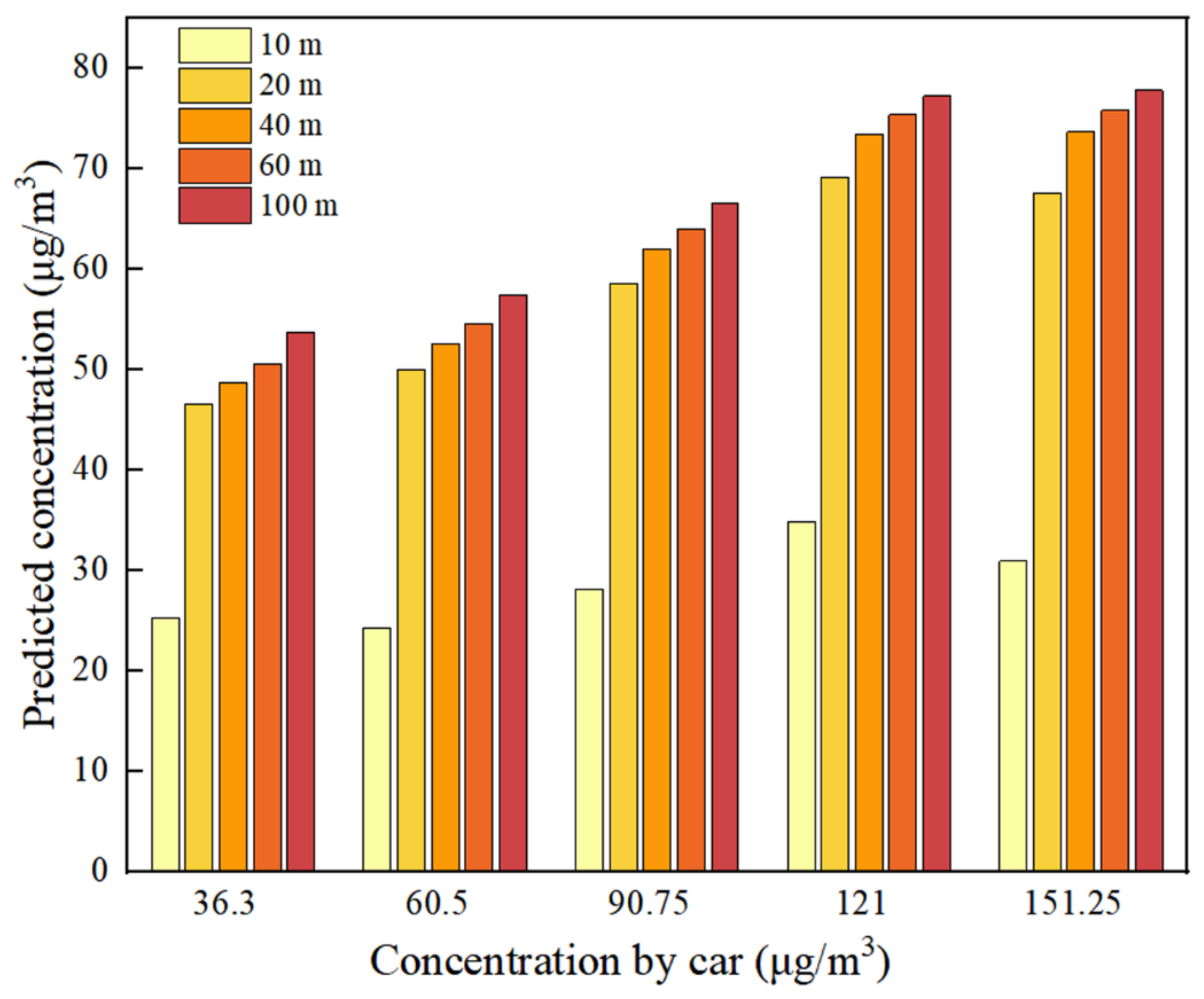
The concentration of traffic-related fine particles during commuting was related to the pollutant concentration discharged by cars. The higher the traffic flow, the higher the pollutant concentration was, and the higher the exposure risk of the commuters was. A 30.25 μg/m³ increase in the C_car resulted in a 7–13 μg/m³ increase in the TRAP concentration on sidewalks.

(2)

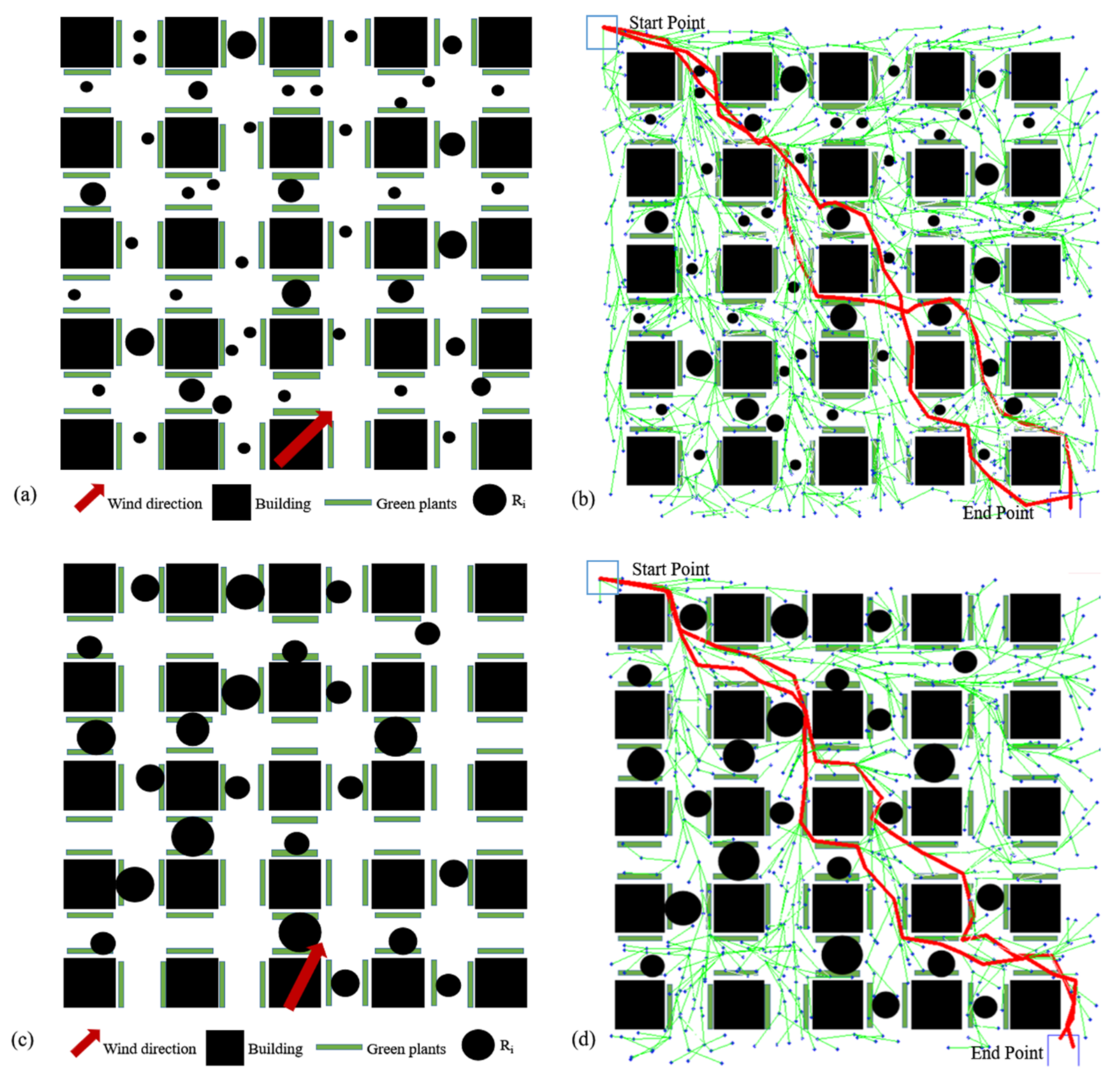
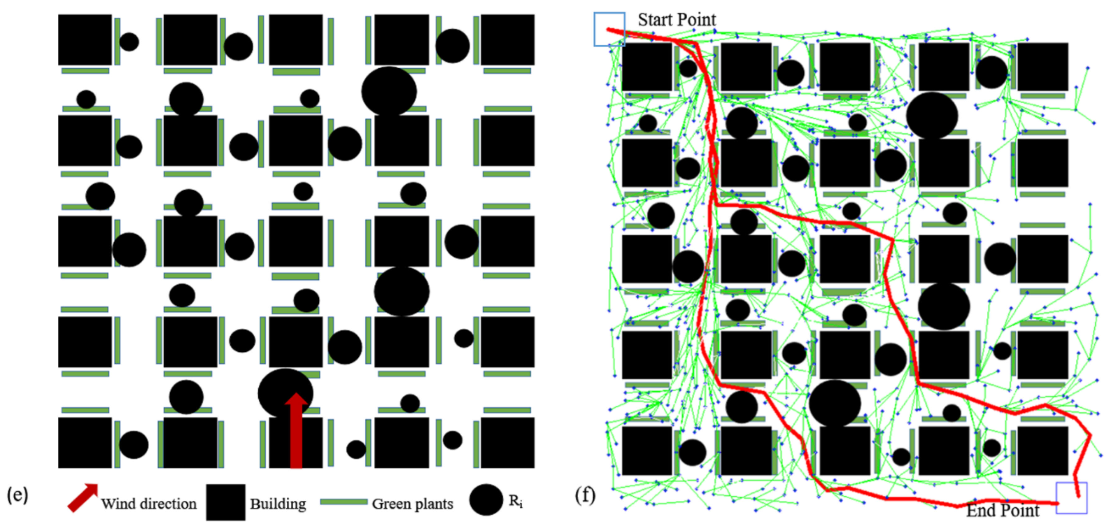
The wind environment significantly affected the pollutant distribution and diffusion. The dilution level of the pollutants influenced by the wind differed for different C_car values, e.g., C_TRAP decreased by about 2.8% for every 2 m/s increase in VEL at the C_car of 90.75 μg/m³. Different wind directions also resulted in different levels of diffusion of traffic-related pollutants, leading to large differences in the pollutant distribution on different routes. The pollutant concentration was low in windy areas, and the pollutants accumulated in the downwind areas of buildings. Therefore, the effects of the wind direction and wind speed should be considered in the design of urban road networks and road direction.

(3)

Vegetation diluted the pollutant concentration. In this study, a large leaf area density significantly reduced the pollutant concentration at the pedestrian level. Therefore, trees with a high leaf area density should be considered for street greening.

(4)

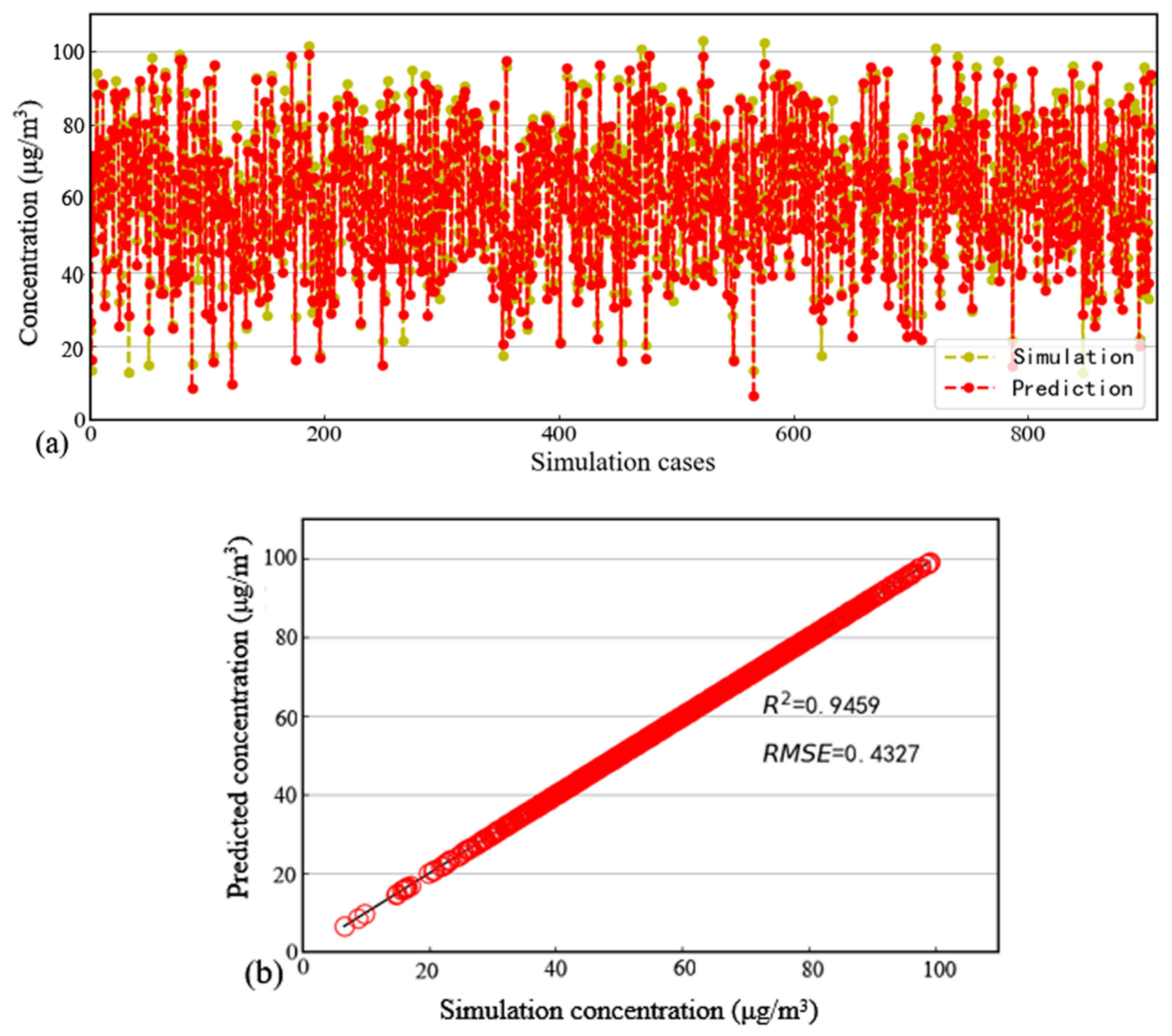
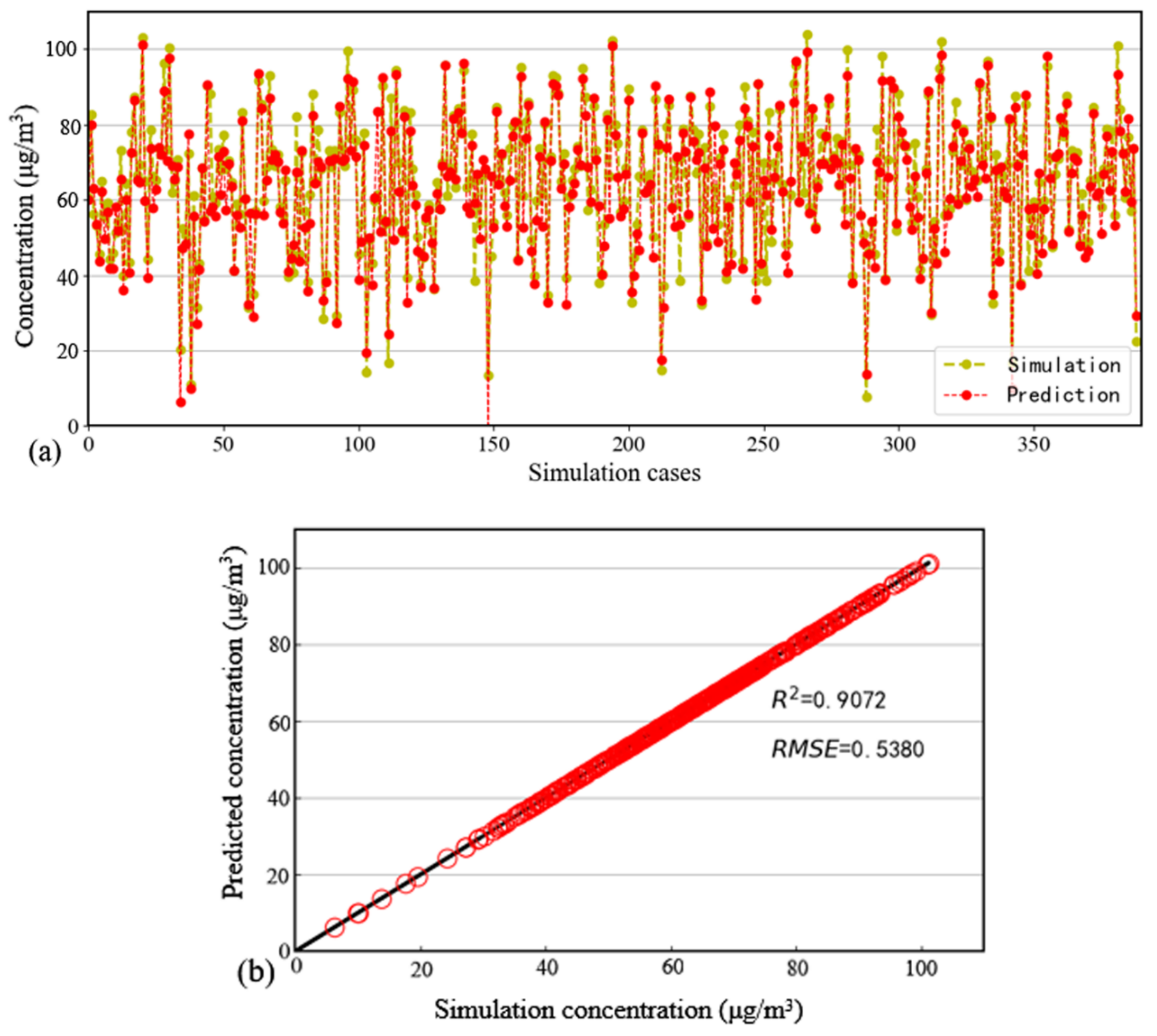
The BP neural network prediction model had a high R² value during training. The results showed that the proposed model could accurately predict the traffic-related particulate matter concentration to provide data for optimizing the commuting routes.

(5)

The BP prediction results were converted into the exposure risk and were mapped to perform commuting path optimization using the RRT* algorithm. The optimum commuter route had the lowest pollution concentration to improve the health of citizens.

References

1. An, F.; Liu, J.; Lu, W.; Jareemit, D. A review of the effect of traffic-related air pollution around schools on student health and its mitigation. J. Transp. Health 2021, 23, 101249. [Google Scholar] [CrossRef]
2. Ji, W.; Zhao, B. Estimating mortality derived from indoor exposure to particles of outdoor origin. PLoS ONE 2015, 10, e0124238. [Google Scholar] [CrossRef] [PubMed]
3. Xiong, R.; Jiang, W.; Li, N.; Liu, B.; He, R.; Wang, B.; Geng, Q. PM2.5-induced lung injury is attenuated in macrophage-specific NLRP3 deficient mice. Ecotoxicol. Environ. Saf. 2021, 221, 112433. [Google Scholar] [CrossRef] [PubMed]
4. Yu, P.; Xu, R.; Li, S.; Coelho, M.S.Z.S.; Saldiva, P.H.N.; Sim, M.R.; Abramson, M.J.; Guo, Y. Associations between long-term exposure to PM2.5 and site-specific cancer mortality: A nationwide study in Brazil between 2010 and 2018. Environ. Pollut. 2022, 302, 119070. [Google Scholar] [CrossRef]
5. Heinzerling, A.; Hsu, J.; Yip, F. Respiratory Health Effects of Ultrafine Particles in Children: A Literature Review. Water Air Soil Pollut. 2016, 227, 32. [Google Scholar] [CrossRef]
6. Alapas, G. Metabolically-Derived Human Ventilation Rates: A Revised Approach Based Upon Oxygen Consumption Rates; US Environmental Protection Agency: Washington, WA, USA, 2009.
7. Bai, L.; Su, X.; Zhao, D.; Zhang, Y.; Cheng, Q.; Zhang, H.; Wang, S.; Xie, M.; Su, H. Exposure to traffic-related air pollution and acute bronchitis in children: Season and age as modifiers. J. Epidemiol. Community Health 2018, 72, 426–433. [Google Scholar] [CrossRef]
8. Basagaña, X.; Esnaola, M.; Rivas, I.; Amato, F.; Alvarez-Pedrerol, M.; Forns, J.; López-Vicente, M.; Pujol, J.; Nieuwenhuijsen, M.; Querol, X.; et al. Neurodevelopmental Deceleration by Urban Fine Particles from Different Emission Sources: A Longitudinal Observational Study. Environ. Health Perspect. 2016, 124, 1630–1636. [Google Scholar] [CrossRef]
9. Beelen, R.; Hoek, G.; Brandt, P.A.v.d.; Goldbohm, R.A.; Fischer, P.; Schouten, L.J.; Jerrett, M.; Hughes, E.; Armstrong, B.; Brunekreef, B. Long-Term Effects of Traffic-Related Air Pollution on Mortality in a Dutch Cohort (NLCS-AIR Study). Environ. Health Perspect. 2008, 116, 196–202. [Google Scholar] [CrossRef]
10. Liu, J.; Cai, W.; Zhu, S.; Dai, F. Impacts of vehicle emission from a major road on spatiotemporal variations of neighborhood particulate pollution—A case study in a university campus. Sustain. Cities Soc. 2020, 53, 101917. [Google Scholar] [CrossRef]
11. Lonati, G.; Ozgen, S.; Ripamonti, G.; Signorini, S. Variability of Black Carbon and Ultrafine Particle Concentration on Urban Bike Routes in a Mid-Sized City in the Po Valley (Northern Italy). Atmosphere 2017, 8, 40. [Google Scholar] [CrossRef]
12. Ahmed, S.; Adnan, M.; Janssens, D.; Wets, G. A route to school informational intervention for air pollution exposure reduction. Sustain. Cities Soc. 2020, 53, 101965. [Google Scholar] [CrossRef]
13. Hinckson, E.A.; Garrett, N.; Duncan, S. Active commuting to school in New Zealand children (2004–2008): A quantitative analysis. Prev. Med. 2011, 52, 332–336. [Google Scholar] [CrossRef]
14. Crawford, S.; Garrard, J. A Combined Impact-Process Evaluation of a Program Promoting Active Transport to School: Understanding the Factors That Shaped Program Effectiveness. Environ. Public Health 2013, 2013, 816961. [Google Scholar] [CrossRef]
15. Briggs, D.J.; de Hoogh, K.; Morris, C.; Gulliver, J. Effects of travel mode on exposures to particulate air pollution. Environ. Int. 2008, 34, 12–22. [Google Scholar] [CrossRef]
16. Gilliland, J.; Maltby, M.; Xu, X.; Luginaah, I.; Loebach, J.; Shah, T. Is active travel a breath of fresh air? Examining children’s exposure to air pollution during the school commute. Spat. Spatio-Temporal Epidemiol. 2019, 29, 51–57. [Google Scholar] [CrossRef]
17. Tang, J.; McNabola, A.; Misstear, B. The potential impacts of different traffic management strategies on air pollution and public health for a more sustainable city: A modelling case study from Dublin, Ireland. Sustain. Cities Soc. 2020, 60, 102229. [Google Scholar] [CrossRef]
18. Chaney, R.A.; Sloan, C.D.; Cooper, V.C.; Robinson, D.R.; Hendrickson, N.R.; Mccord, T.A.; Johnston, J.D.; Coulombe, R.A. Personal exposure to fine particulate air pollution while commuting: An examination of six transport modes on an urban arterial roadway. PLoS ONE 2017, 12, e0188053. [Google Scholar] [CrossRef]
19. Hang, J.; Li, Y. Ventilation strategy and air change rates in idealized high-rise compact urban areas. Build. Environ. 2010, 45, 2754–2767. [Google Scholar] [CrossRef]
20. Hang, J.; Li, Y.; Sandberg, M.; Buccolieri, R.; Di Sabatino, S. The influence of building height variability on pollutant dispersion and pedestrian ventilation in idealized high-rise urban areas. Build. Environ. 2012, 56, 346–360. [Google Scholar] [CrossRef]
21. Hang, J.; Sandberg, M.; Li, Y. Age of air and air exchange efficiency in idealized city models. Build. Environ. 2009, 44, 1714–1723. [Google Scholar] [CrossRef]
22. Kato, S.; Ito, K.; Murakami, S. Analysis of visitation frequency through particle tracking method based on LES and model experiment. Indoor Air 2003, 13, 182–193. [Google Scholar] [CrossRef]
23. Li, X.-X.; Liu, C.-H.; Leung, D.Y.C. Numerical investigation of pollutant transport characteristics inside deep urban street canyons. Atmos. Environ. 2009, 43, 2410–2418. [Google Scholar] [CrossRef]
24. Lim, E.; Ito, K.; Sandberg, M. New ventilation index for evaluating imperfect mixing conditions–Analysis of Net Escape Velocity based on RANS approach. Build. Environ. 2013, 61, 45–56. [Google Scholar] [CrossRef]
25. Meroney, R.N.; Pavageau, M.; Rafailidis, S.; Schatzmann, M. Study of line source characteristics for 2-D physical modelling of pollutant dispersion in street canyons. J. Wind Eng. Ind. Aerodyn. 1996, 62, 37–56. [Google Scholar] [CrossRef]
26. Mirzaei, P.A.; Haghighat, F. Pollution removal effectiveness of the pedestrian ventilation system. J. Wind Eng. Ind. Aerodyn. 2011, 99, 46–58. [Google Scholar] [CrossRef]
27. Oke, T.R. Street design and urban canopy layer climate. Energy Build. 1988, 11, 103–113. [Google Scholar] [CrossRef]
28. Li, Q.; Liang, J.; Wang, Q.; Chen, Y.; Yang, H.; Ling, H.; Luo, Z.; Hang, J. Numerical Investigations of Urban Pollutant Dispersion and Building Intake Fraction with Various 3D Building Configurations and Tree Plantings. Int. J. Environ. Res. Public Health 2022, 19, 3524. [Google Scholar] [CrossRef]
29. Chang, C.-H.; Meroney, R.N. Concentration and flow distributions in urban street canyons: Wind tunnel and computational data. J. Wind Eng. Ind. Aerodyn. 2003, 91, 1141–1154. [Google Scholar] [CrossRef]
30. Chew, L.W.; Aliabadi, A.A.; Norford, L.K. Flows across high aspect ratio street canyons: Reynolds number independence revisited. Environ. Fluid Mech. 2018, 18, 1275–1291. [Google Scholar] [CrossRef]
31. Li, X.-X.; Liu, C.-H.; Leung, D.Y.C.; Lam, K.M. Recent progress in CFD modelling of wind field and pollutant transport in street canyons. Atmos. Environ. 2006, 40, 5640–5658. [Google Scholar] [CrossRef]
32. Tominaga, Y.; Stathopoulos, T. CFD simulation of near-field pollutant dispersion in the urban environment: A review of current modeling techniques. Atmos. Environ. 2013, 79, 716–730. [Google Scholar] [CrossRef]
33. Bady, M.; Kato, S.; Huang, H. Towards the application of indoor ventilation efficiency indices to evaluate the air quality of urban areas. Build. Environ. 2008, 43, 1991–2004. [Google Scholar] [CrossRef]
34. Viotti, P.; Liuti, G.; Di Genova, P. Atmospheric urban pollution: Applications of an artificial neural network (ANN) to the city of Perugia. Ecol. Model. 2002, 148, 27–46. [Google Scholar] [CrossRef]
35. Blocken, B. 50 years of Computational Wind Engineering: Past, present and future. J. Wind Eng. Ind. Aerodyn. 2014, 129, 69–102. [Google Scholar] [CrossRef]
36. Liu, J.; Heidarinejad, M.; Pitchurov, G.; Zhang, L.; Srebric, J. An extensive comparison of modified zero-equation, standard k-ε, and LES models in predicting urban airflow. Sustain. Cities Soc. 2018, 40, 28–43. [Google Scholar] [CrossRef]
37. Gao, Z.; Bresson, R.; Qu, Y.; Milliez, M.; de Munck, C.; Carissimo, B. High resolution unsteady RANS simulation of wind, thermal effects and pollution dispersion for studying urban renewal scenarios in a neighborhood of Toulouse. Urban Clim. 2018, 23, 114–130. [Google Scholar] [CrossRef]
38. Wang, W.; Ng, E. Air ventilation assessment under unstable atmospheric stratification—A comparative study for Hong Kong. Build. Environ. 2018, 130, 1–13. [Google Scholar] [CrossRef]
39. Srebric, J.; Heidarinejad, M.; Liu, J. Building neighborhood emerging properties and their impacts on multi-scale modeling of building energy and airflows. Build. Environ. 2015, 91, 246–262. [Google Scholar] [CrossRef]
40. Liu, J.; Zhang, X.; Niu, J.; Tse, K.T. Pedestrian-level wind and gust around buildings with a ‘lift-up’ design: Assessment of influence from surrounding buildings by adopting LES. Build. Simul. 2019, 12, 1107–1118. [Google Scholar] [CrossRef]
41. Yang, H.; Lam, C.K.C.; Lin, Y.; Chen, L.; Mattsson, M.; Sandberg, M.; Hayati, A.; Claesson, L.; Hang, J. Numerical investigations of Re-independence and influence of wall heating on flow characteristics and ventilation in full-scale 2D street canyons. Build. Environ. 2021, 189, 107510. [Google Scholar] [CrossRef]
42. Liu, J.; Heidarinejad, M.; Nikkho, S.K.; Mattise, N.W.; Srebric, J. Quantifying Impacts of Urban Microclimate on a Building Energy Consumption—A Case Study. Sustainability 2019, 11, 4921. [Google Scholar] [CrossRef]
43. Blocken, B. LES over RANS in building simulation for outdoor and indoor applications: A foregone conclusion? Build. Simul. 2018, 11, 821–870. [Google Scholar] [CrossRef]
44. Liu, J.; Srebric, J.; Yu, N. Numerical simulation of convective heat transfer coefficients at the external surfaces of building arrays immersed in a turbulent boundary layer. Int. J. Heat Mass Transf. 2013, 61, 209–225. [Google Scholar] [CrossRef]
45. Liu, J.; Heidarinejad, M.; Gracik, S.; Srebric, J. The impact of exterior surface convective heat transfer coefficients on the building energy consumption in urban neighborhoods with different plan area densities. Energy Build. 2015, 86, 449–463. [Google Scholar] [CrossRef]
46. Cui, D.; Hu, G.; Ai, Z.; Du, Y.; Mak, C.M.; Kwok, K. Particle image velocimetry measurement and CFD simulation of pedestrian level wind environment around U-type street canyon. Build. Environ. 2019, 154, 239–251. [Google Scholar] [CrossRef]
47. Panagiotou, I.; Neophytou, M.K.A.; Hamlyn, D.; Britter, R.E. City breathability as quantified by the exchange velocity and its spatial variation in real inhomogeneous urban geometries: An example from central London urban area. Sci. Total Environ. 2013, 442, 466–477. [Google Scholar] [CrossRef]
48. Wang, W.; Xu, Y.; Ng, E.; Raasch, S. Evaluation of satellite-derived building height extraction by CFD simulations: A case study of neighborhood-scale ventilation in Hong Kong. Landsc. Urban Plan. 2018, 170, 90–102. [Google Scholar] [CrossRef]
49. Van Hooff, T.; Blocken, B. On the effect of wind direction and urban surroundings on natural ventilation of a large semi-enclosed stadium. Comput. Fluids 2010, 39, 1146–1155. [Google Scholar] [CrossRef]
50. Montazeri, H.; Blocken, B.; Janssen, W.D.; van Hooff, T. CFD evaluation of new second-skin facade concept for wind comfort on building balconies: Case study for the Park Tower in Antwerp. Build. Environ. 2013, 68, 179–192. [Google Scholar] [CrossRef]
51. Toparlar, Y.; Blocken, B.; Vos, P.; van Heijst, G.J.F.; Janssen, W.D.; van Hooff, T.; Montazeri, H.; Timmermans, H.J.P. CFD simulation and validation of urban microclimate: A case study for Bergpolder Zuid, Rotterdam. Build. Environ. 2015, 83, 79–90. [Google Scholar] [CrossRef]
52. Li, J.; Liu, J.; Srebric, J.; Hu, Y.; Liu, M.; Su, L.; Wang, S. The Effect of Tree-Planting Patterns on the Microclimate within a Courtyard. Sustainability 2019, 11, 1665. [Google Scholar] [CrossRef]
53. Zhang, K.; Chen, G.; Zhang, Y.; Liu, S.; Wang, X.; Wang, B.; Hang, J. Integrated impacts of turbulent mixing and NOX-O3 photochemistry on reactive pollutant dispersion and intake fraction in shallow and deep street canyons. Sci. Total Environ. 2020, 712, 135553. [Google Scholar] [CrossRef] [PubMed]
54. Chen, L.; Hang, J.; Sandberg, M.; Claesson, L.; Di Sabatino, S.; Wigo, H. The impacts of building height variations and building packing densities on flow adjustment and city breathability in idealized urban models. Build. Environ. 2017, 118, 344–361. [Google Scholar] [CrossRef]
55. Lin, Y.; Chen, G.; Chen, T.; Luo, Z.; Yuan, C.; Gao, P.; Hang, J. The influence of advertisement boards, street and source layouts on CO dispersion and building intake fraction in three-dimensional urban-like models. Build. Environ. 2019, 150, 297–321. [Google Scholar] [CrossRef]
56. Lin, B.; Li, X.; Zhu, Y.; Qin, Y. Numerical simulation studies of the different vegetation patterns’ effects on outdoor pedestrian thermal comfort. J. Wind Eng. Ind. Aerodyn. 2008, 96, 1707–1718. [Google Scholar] [CrossRef]
57. Qin, H.; Hong, B.; Jiang, R.; Yan, S.; Zhou, Y. The Effect of Vegetation Enhancement on Particulate Pollution Reduction: CFD Simulations in an Urban Park. Forests 2019, 10, 373. [Google Scholar] [CrossRef]
58. Green, S.R. Modelling Turbulent Air Flow in a Stand of Widely-Spaced Trees. PHOENICS J. Comput. Fluid Dyn. Its Appl. 1992, 5, 294–312. [Google Scholar]
59. Ji, W.; Zhao, B. Numerical study of the effects of trees on outdoor particle concentration distributions. Build. Simul.-China 2014, 7, 417–427. [Google Scholar] [CrossRef]
60. Nowak, D.J.; Hirabayashi, S.; Bodine, A.; Hoehn, R. Modeled PM2.5 removal by trees in ten U.S. cities and associated health effects. Environ. Pollut. 2013, 178, 395–402. [Google Scholar] [CrossRef]
61. Sha, C.; Wang, X.; Lin, Y.; Fan, Y.; Chen, X.; Hang, J. The impact of urban open space and ‘lift-up’ building design on building intake fraction and daily pollutant exposure in idealized urban models. Sci. Total Environ. 2018, 633, 1314–1328. [Google Scholar] [CrossRef]
62. Tominaga, Y.; Mochida, A.; Yoshie, R.; Kataoka, H.; Nozu, T.; Yoshikawa, M.; Shirasawa, T. AIJ guidelines for practical applications of CFD to pedestrian wind environment around buildings. J. Wind Eng. Ind. Aerodyn. 2008, 96, 1749–1761. [Google Scholar] [CrossRef]
63. Su, M.; Liu, J.; Zhou, S.; Miao, J.; Kim, M.K. Dynamic prediction of the pre-dehumidification of a radiant floor cooling and displacement ventilation system based on computational fluid dynamics and a back-propagation neural network: A case study of an office room. Indoor Built Environ. 2022; in press. [Google Scholar] [CrossRef]
64. Kim, M.K.; Cremers, B.; Liu, J.; Zhang, J.; Wang, J. Prediction and correlation analysis of ventilation performance in a residential building using artificial neural network models based on data-driven analysis. Sustain. Cities Soc. 2022, 83, 103981. [Google Scholar] [CrossRef]
65. Tasadduq, I.; Rehman, S.; Bubshait, K. Application of neural networks for the prediction of hourly mean surface temperatures in Saudi Arabia. Renew. Energy 2002, 25, 545–554. [Google Scholar] [CrossRef]
66. Ren, L.; Liu, Y.; Rui, Z.; Li, H.; Feng, R. Application of Elman Neural Network and MATLAB to Load Forecasting. In Proceedings of the 2009 International Conference on Information Technology and Computer Science, Kiev, Ukraine, 25–26 July 2009; pp. 55–59. [Google Scholar]
67. Mohanraj, M.; Jayaraj, S.; Muraleedharan, C. Applications of artificial neural networks for refrigeration, air-conditioning and heat pump systems—A review. Renew. Sustain. Energy Rev. 2012, 16, 1340–1358. [Google Scholar] [CrossRef]
68. Nasruddin; Sholahudin; Satrio, P.; Mahlia, T.M.I.; Giannetti, N.; Saito, K. Optimization of HVAC system energy consumption in a building using artificial neural network and multi-objective genetic algorithm. Sustain. Energy Technol. Assess. 2019, 35, 48–57. [Google Scholar] [CrossRef]
69. Qi, A. Research on Prediction Model of Improved BP Neural Network Optimized by Genetic Algorithm. In Proceedings of the 2017 4th International Conference on Machinery, Materials and Computer (MACMC 2017), Xi’an, China, 27–29 November 2017; pp. 764–767. [Google Scholar]
70. Hinds, W.C.; Zhu, Y. Aerosol Technology: Properties, Behavior, and Measurement of Airborne Particles; John Wiley & Sons: New York, NJ, USA, 1982. [Google Scholar]
71. Kwiecień, J.; Szopińska, K. Mapping Carbon Monoxide Pollution of Residential Areas in a Polish City. Remote Sens. 2020, 12, 2885. [Google Scholar] [CrossRef]
72. Gu, Z.-L.; Zhang, Y.-W.; Cheng, Y.; Lee, S.-C. Effect of uneven building layout on air flow and pollutant dispersion in non-uniform street canyons. Build. Environ. 2011, 46, 2657–2665. [Google Scholar] [CrossRef]
73. Fenger, J. Urban air quality. Atmos. Environ. 1999, 33, 4877–4900. [Google Scholar] [CrossRef]
74. Chan, C.K.; Yao, X. Air pollution in mega cities in China. Atmos. Environ. 2008, 42, 1–42. [Google Scholar] [CrossRef]
75. An, F.; Liu, J.; Lu, W.; Jareemit, D. Comparison of exposure to traffic-related pollutants on different commuting routes to a primary school in Jinan, China. Environ. Sci. Pollut. Res. Int. 2022, 29, 43319–43340. [Google Scholar] [CrossRef]
76. Kumar, P.; Rivas, I.; Sachdeva, L. Exposure of in-pram babies to airborne particles during morning drop-in and afternoon pick-up of school children. Environ. Pollut. 2017, 224, 407–420. [Google Scholar] [CrossRef]
77. Garcia-Algar, O.; Canchucaja, L.; d’Orazzio, V.; Manich, A.; Joya, X.; Vall, O. Different exposure of infants and adults to ultrafine particles in the urban area of Barcelona. Environ. Monit. Assess. 2014, 187, 4196. [Google Scholar] [CrossRef]
Figure 1. Flowchart of this study.
Buildings 12 01227 g001
Figure 2. Geometric model of the CFD simulation. (a) The computational domain of case I: BH = 10 m, FAR = 0.75; (b) 3D urban models for cases I, II, and III; (c) the buildings, trees, and pollutant sources.
Buildings 12 01227 g002
Figure 3. The two routes of the simulation validation.
Buildings 12 01227 g003
Figure 4. Numerical simulation results of PM2.5 concentration. (a) Case 1; (b) case 2.
Buildings 12 01227 g004
Figure 5. Comparison of measured values and simulation values for validation case 1.
Buildings 12 01227 g005
Figure 6. Comparison of measured values and simulation values for validation case 2.
Buildings 12 01227 g006
Figure 7. Structure of the BP neural network model.
Buildings 12 01227 g007
Figure 8. The flowchart of the BP neural network.
Buildings 12 01227 g008
Figure 9. Schematic of calculating the values of respiratory deposition dose at different points.
Buildings 12 01227 g009
Figure 10. Selection of the sample points using Python.
Buildings 12 01227 g010
Figure 11. The pollutant concentrations for different wind speeds in FAR II. (a) VEL = 3 m/s, Ccar = 90.75 μg/m3, (b) VEL = 3 m/s, Ccar = 121.00 μg/m3, (c) VEL = 3 m/s, Ccar = 151.25 μg/m3, (d) VEL = 5 m/s, Ccar = 90.75 μg/m3, (e) VEL = 5 m/s, Ccar = 121.00 μg/m3, (f) VEL = 5 m/s, Ccar = 151.25 μg/m3, (g) VEL = 7 m/s, Ccar = 90.75 μg/m3, (h) VEL = 7 m/s, Ccar = 121.00 μg/m3, and (i) VEL = 7 m/s, Ccar = 151.25 μg/m3.
Buildings 12 01227 g011
Figure 12. PM2.5 distributions in different wind directions of FAR II, VEL = 3 m/s, Ccar = 151.25 μg/m3. (a) VDR = 180°, (b) VDR = 195°, (c) VDR = 210°, and (d) VDR = 225°.
Buildings 12 01227 g012
Figure 13. The concentrations of pollutants for different LADs in circle of FAR II, VEL = 3 m/s. (a) Ccar = 90.75 μg/m3, LAD = 1.0, (b) Ccar = 90.75 μg/m3, LAD = 4.0, (c) Ccar = 121.00 μg/m3, LAD = 1.0, (d) Ccar = 121.00 μg/m3, LAD = 4.0, (e) Ccar = 151.25 μg/m3, LAD = 1.0, and (f) Ccar = 151.25 μg/m3, LAD = 4.0.
Buildings 12 01227 g013
Figure 14. The pollutant concentrations for different background concentrations and FAR Ⅱ, VEL = 1 m/s, and VDR = 180°. (a) Cback = 12.10 μg/m3, (b) Cback = 36.30 μg/m3, and (c) Cback = 60.50 μg/m3.
Buildings 12 01227 g014
Figure 15. The training results of the BP neural network for predicting the TRAP concentration: (a) comparison of the simulation and prediction results; (b) predicted versus simulated values.
Buildings 12 01227 g015
Figure 16. The validation results of the BP neural network for predicting the TRAP concentration: (a) comparison of the simulation and prediction results; (b) predicted versus simulated values.
Buildings 12 01227 g016
Figure 17. Predicted concentration for different building heights and Ccar.
Buildings 12 01227 g017
Figure 18. Optimal paths for different cases of FAR I: Cback = 60.50 μg/m3, VEL = 1 m/s, LAD = 4.0, and Ccar = 36.30~151.25 μg/m3. (a) VDR = 225°, (b) optimal path for VDR = 225°, (c) VDR = 195°, (d) optimal path for VDR = 195°, (e) VDR = 180°, and (f) optimal path for VDR = 180°. The red lines represent the optimal paths obtained from the RRT* algorithm.
Buildings 12 01227 g018aBuildings 12 01227 g018b