The Influence of Block Morphology on Urban Thermal Environment Analysis Based on a Feed-Forward Neural Network Model

Abstract

Morphological indicators, which are important for urban planning, can be adjusted to effectively mitigate the heat island effect and promote a more comfortable urban environment. Most studies obtain the relationship between morphological indicators and land surface temperature (LST) from the urban scale, and it is difficult to apply the results to urban management and construction projects. Traditional research methods have ignored the complex and interactive relationship between morphological indicators and LST. In this work, the feed-forward neural network (FNN) model is utilized to model the nonlinear relationship between morphological indicators and LST at the block scale. After validation and comparison, the FNN model achieved MAE of 0.885 and RMSE of 1.184, indicating that the influence of morphological indicators on LST could be precisely mapped. In addition, using cooling LST as the optimization target, the specific indicator scheme is suggested based on the FNN model, where the percentage of green space is 17.1%, the percentage of impervious surface is 82.9%, the percentage of water is 0, the bare soil percentage is 0, the floor area ratio is 0.814, the building cover percentage is 32.2%, and the average building height is 7.2 m.

1. Introduction

Urban heat islands (UHIs) are a worldwide phenomenon in which urban areas tend to have a higher land surface temperature (LST) or air temperature than the surrounding rural areas [1]. The causes of the higher temperatures in urban areas include changes in land use, such as an increasing number of artificial constructions and a decrease in green spaces and water areas, as well as an increase in population heat emissions. As a result, the number of uncomfortable tropical nights and the incidence of heat illnesses have increased, and various other effects have resulted in the loss of a comfortable living environment [2,3,4]. Therefore, encouraging sustainable national and urban development requires consciously addressing these difficult problems that involve citizens’ health and electricity use by reducing the urban heat island effect [5].

The thermal environment of the city can be controlled through surface temperature and canopy temperature, which together make up the multilayered structure of the urban climate [6]. The surface heat island effect is used to characterize this effect [7]. Canopy air temperature is derived mainly from measured air temperature data collected by urban weather stations or mobile vehicles and is widely used [8]. Given that a significant number of studies worldwide have used air and surface temperatures to explore the spatial and temporal characteristics and drivers of the urban thermal environment at the horizontal level, LST has the obvious advantage of being able to correspond well to urban space at the whole urban spatial scale. The urban surface layer is typically described using a variety of surface parameters, including vegetation cover, impervious area, area of water bodies, etc. [9]. Lu, Yue, and Huang (2021) examined the impact of land use on LST while using LST to characterize the distribution of the urban thermal environment [5]. Analyzing the impact of land use on the LST, the LST was used to characterize the distribution of the urban thermal environment.

Urban thermal environment research concentrates on the variations in LST distribution within urban built-up areas due to differences in spatial organization, land use, development intensity, and three-dimensional spatial structure. In order to investigate the relationship between urban space and the thermal environment, Ref. [10] introduced the concept of urban zoning (local climate zones). This approach forms homogeneous units with consistent land cover, spatial structure, building materials, and human activity patterns [11,12]. Since the suggested measures or strategies are challenging to incorporate into actual urban planning, these studies focus on the macro level, considering individual cities as a whole, but ignoring the internal spatial heterogeneity of their urban spaces. The block is the smallest unit in the urban planning system where the local government uses zoning to control land. Morphological indicators are one of the key factors in urban planning [13]; measures proposed at the block scale that would contribute to the change in the urban thermal environment can be applied more specifically in urban planning. In order to explore the connection between the land use situation and the urban thermal environment, the study of land cover is more frequently conducted in terms of cities, where the entire area is extracted or different functional areas of buildings are classified [14]. Adjusting the block factor links for thermal environment issues is difficult and less operable, because this ignores the scale and spatial–geographic relationships of urban blocks. It is proposed that the control unit zoning method be used to investigate the relationship between LST and morphological indicators [15,16].

The main methods used to study the influence of block morphological indicators on the urban thermal environment focus on the use of linear regression [9,17] and geospatially weighted models [15]. Moreover, the relationship between the effect of morphological indicators on the thermal environment or thermal comfort is obtained using thermal environment simulations that control for a single variable of morphological indicators [18]. These studies have ignored the relationships between morphological indicators that affect one another in order to investigate the effects of morphological indicators on the thermal environment using independent linear models. The relationship between these urban morphological indexes and the thermal environment is not a direct mathematical expression, and therefore, traditional optimization methods based on functional expressions cannot be used—instead, intelligent algorithms are preferred [19]. Artificial neural network (ANN) is an unconventional modeling strategy that can effectively fit multivariate input and output processes. It can infinitely approximate any nonlinear continuous function with any deterministic accuracy, thanks to its powerful nonlinear simulation capability; by combining all the indicators, it can perform a systematic and thorough evaluation. The urban environment itself has a high level of complexity, and machine learning is better at performing non-linear analysis than traditional regression methods [20]. ANNs have been applied in various urban studies to solve meteorology-related problems [21,22], predict urban land use and scale development [23,24], and predict urban air quality [25]. Feed-forward neural networks (FNN) have begun to be used extensively in urban planning and construction as a result of the development of big data, the Internet of Things, cloud computing, and other related technologies [26].

This study proposes a method to analyze and optimize the thermal environment by dividing block units. Kitakyushu was used as the research area, and multiple sources of data were used to obtain the morphological indexes and LST distribution characteristics of each unit. Kitakyushu is the second largest city on Kyushu Island after Fukuoka, and has an excellent geographical location. Since Kitakyushu has begun to adjust its urban planning to the goal of livability, this study is useful in providing new ideas for urban planning in Kitakyushu, as well as for similar cities in Japan. Following that, the FNN model was utilized to model the relationship between block morphological indicators and LST, and the distribution characteristics of the urban thermal environment and the sensitive areas of local heat islands were identified. For a typical block, a control strategy to lessen the indicators of the urban thermal environment was suggested. The following three aspects are the main contributions of this study:

• We suggest using the road network information to divide the blocks based on the current urban built-up situation and planning in order to explore the specific measures to control the block shape indexes that can be used to inform urban planning.
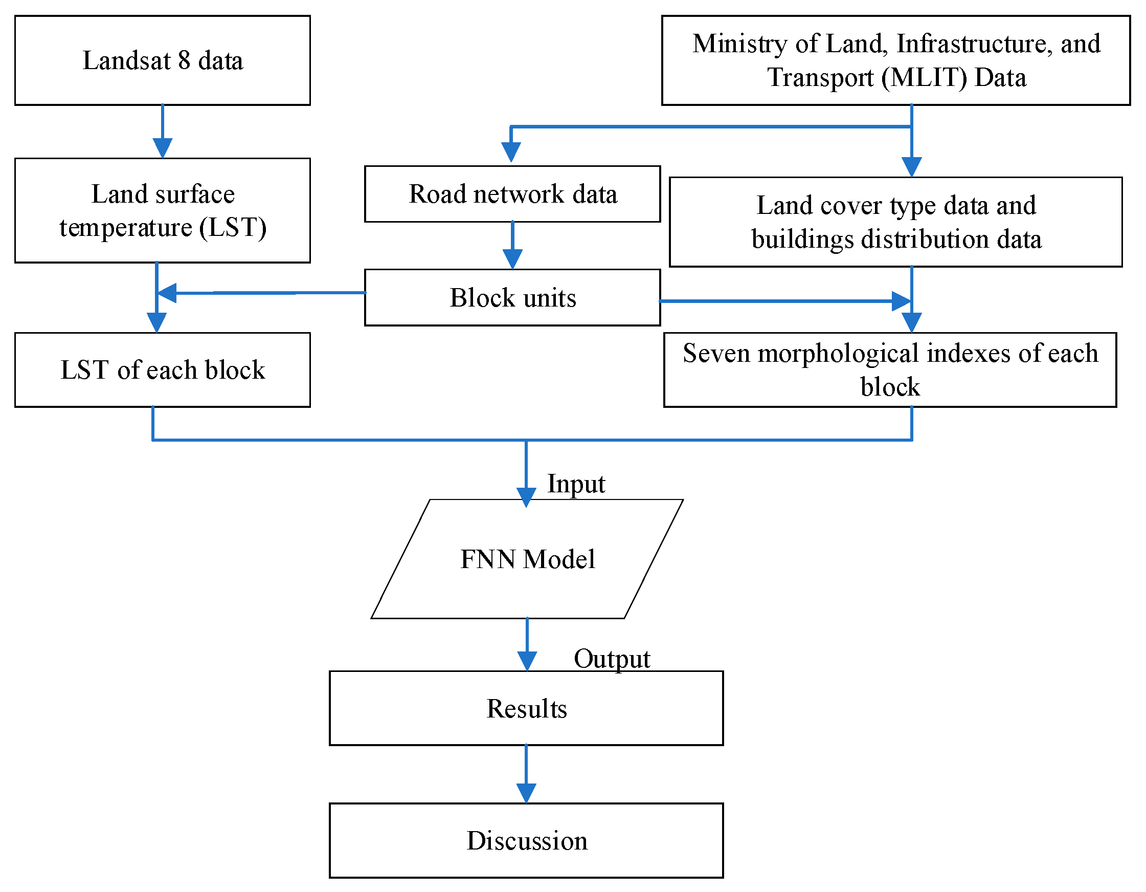
• We empirically study the construction of block morphological indicators and land surface temperature based on a feed-forward neural network model.
• We provide a feed-forward neural network model application to adjust the block morphological indicators with cooling LST as the optimization target.

2. Construction of the Feed-Forward Neural Network Model

Based on the above problems, we modeled the nonlinear relationship between morphological indicators and LST from the block scale using the FNN model and performed block indicator optimization with the validated model. The specific workflow of this study is shown in Figure 1 and can be divided into three parts. (1) Taking Kitakyushu, Japan, as the research area, the city was divided into 373 block-scale units using the current scale of the urban road network. (2) The morphological indicators and LST data of each block are calculated by combining the current building distribution and land use status to construct the dataset. (3) The pre-processed morphological indexes and LST datasets of each block were used to construct an FNN model to explore the nonlinear relationship between morphological indexes and the urban thermal environment.

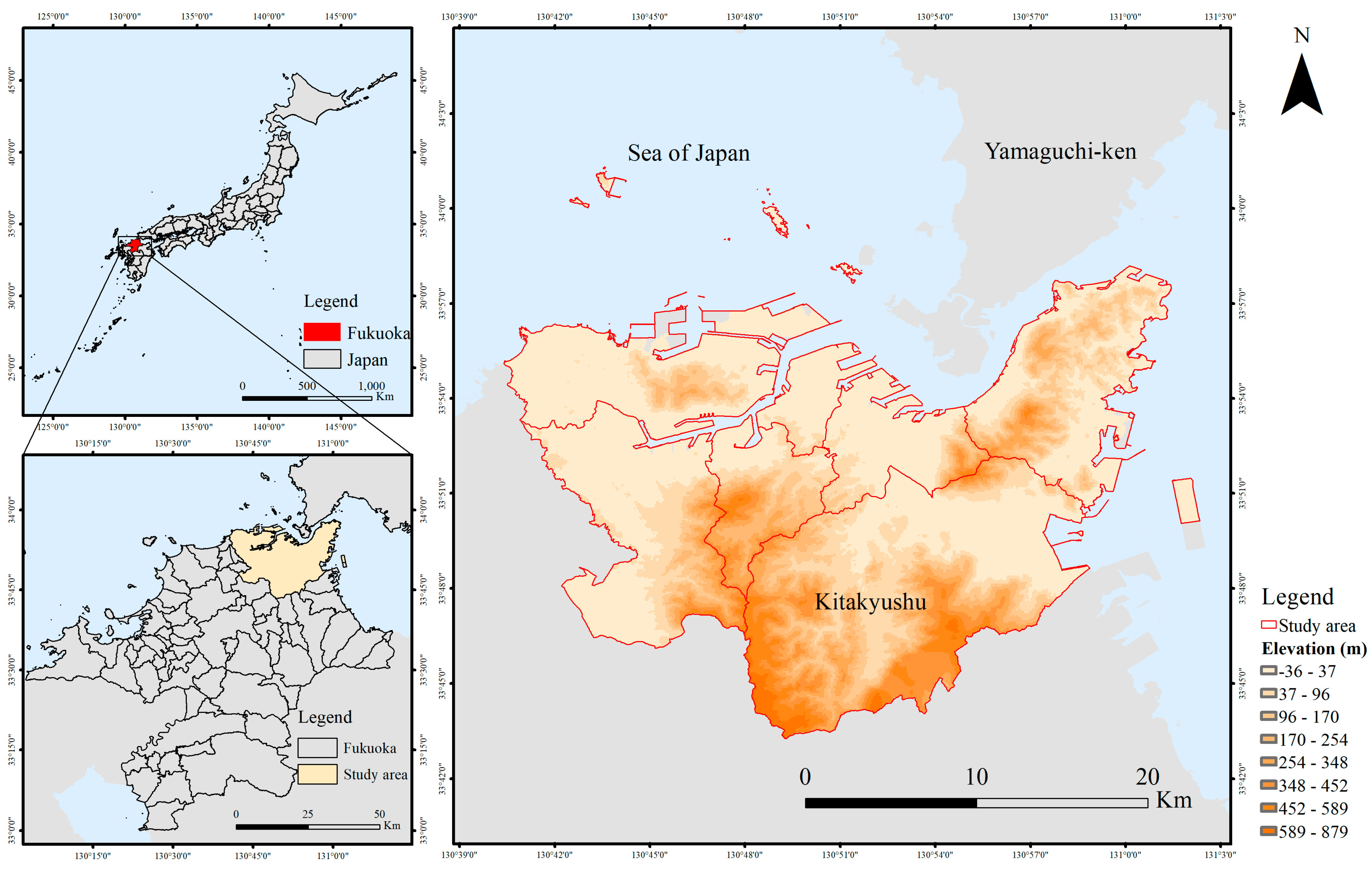
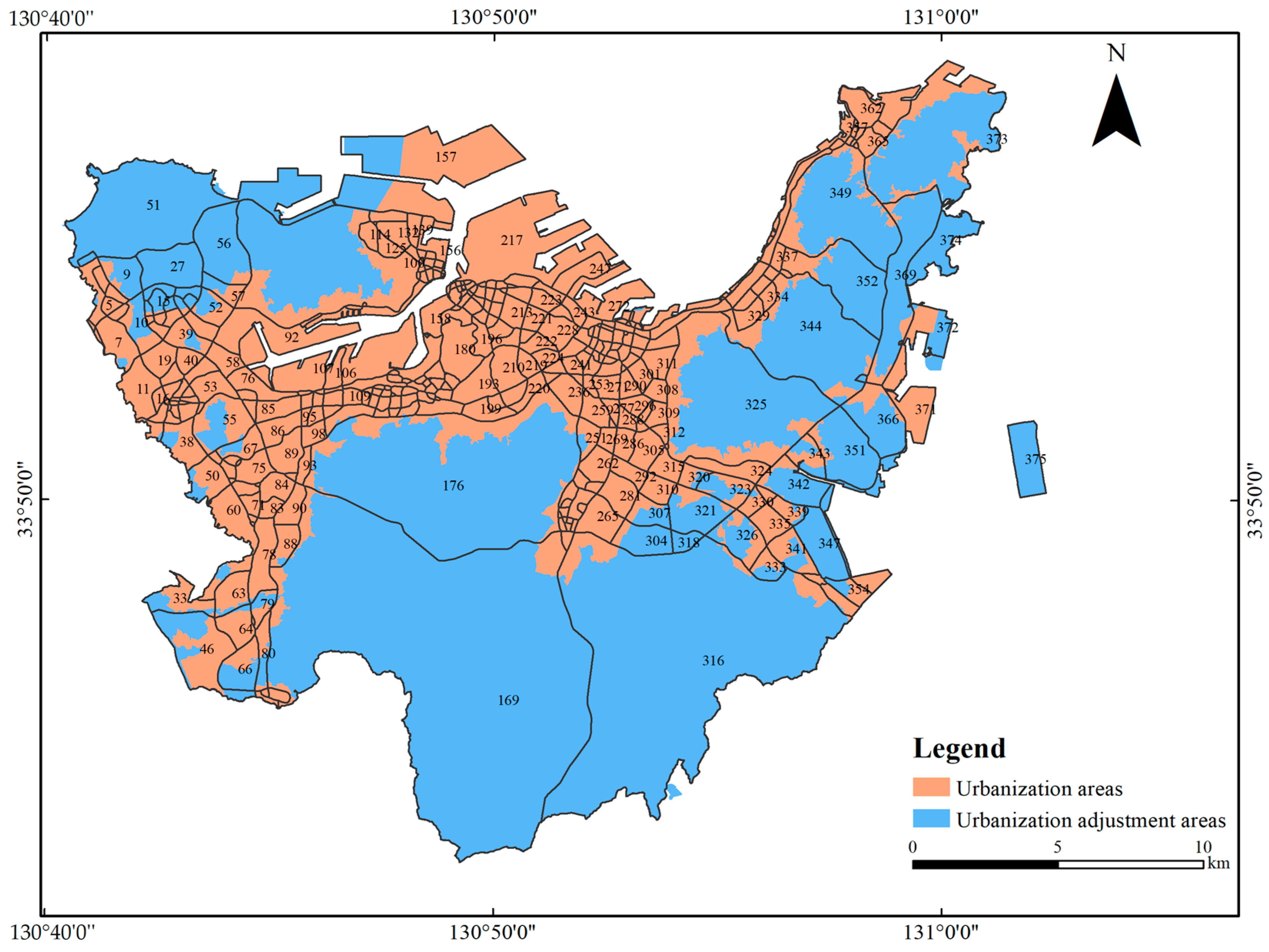
2.1. Study Area and Data

Kitakyushu belongs to Fukuoka Ken, Japan, 130°52′ E, 33°53′ N, with an area of 486.81 km², located in the Kanmon Strait at the northernmost point of Kyushu Island. Fukuoka–Kitakyushu metropolitan area is the fourth largest metropolitan area after Tokyo, Osaka, and Nagoya [27]. It is separated from Honshu Island and opposite to Shimonoseki City, which is a major port city in Japan. With a population of about 970,000, Kitakyushu is the second largest city in Fukuoka Ken and Kyushu Island after Fukuoka. It is one of the twenty designated cities in Japan and one of the three designated cities in Kyushu. Kitakyushu consists of seven wards: Moji, Kokurakita, Kokuraminami, Wakamatsu, Yawatanishi, Yawatahigashi, and Tobata. The geographical location of the study area is shown in Figure 2.

Kitakyushu has a mild and humid climate, with mild winters and hot, humid, and rainy summers. Like the other regions of Japan, the city is subject to the influence of monsoonal circulation: cold northwestern currents prevail in the winter, while the summer is affected by hot and humid air currents from the tropics. The monthly temperature distribution for the past 30 years is shown in Figure 3. In the past century, the city shrank due to rapid industrial development followed by a national economic downturn. The city of Kitakyushu initiated an urban revitalization model in the 1950s with the aim of changing the urban environment and developing Kitakyushu’s full potential by taking advantage of the city’s location in the center of East Asia as well as its accumulated manufacturing capacity. The rational use of the city’s green and coastal resources to create a livable living environment was one of the main goals of the Kitakyushu Urban Master Plan. Therefore, this study can provide strategies for urban planning in Kitakyushu to develop a more comfortable urban environment.

To analyze land use in Kitakyushu, the data of the National Land Numerical Information of the Ministry of Land, Infrastructure, and Transport (MLIT) were used. The National Land Numerical Information comprises GIS data that provide basic information on national land, such as topography, land use, and public facilities, in order to contribute to the promotion of national land policies such as national land formation plans and national land use plans. The data are based on the current status survey in 2015, and the vector files of the road network, building status, and land use were formed with the coordinate system JGD_2000_JAPAN. There are 23 different types of land use, and four different types of land can be created by combining other types of land: impervious land, bare land, water body, and green land. The building status vector file includes the building height and area of the buildings on the ground. In this study, Arc GIS was used to calculate the morphological indicators in each block unit. According to the urban plan of Kitakyushu City, it is divided into urbanization areas and urbanization adjustment areas (Figure 4). Urbanization areas refer to priority and planned urbanization, and urbanization adjustment areas refer to areas where urbanization is controlled and development and construction are prohibited, in principle. In this study, the road network of Kitakyushu was used to divide the block units, and the road vector data were also obtained from the MLIT. The block units of the study area after division are shown in Figure 4. The total number of block units was 373, of which 282 units were located in urbanization areas and 91 units in urbanization adjustment areas. These units cover the built-up area of Kitakyushu with a variety of block patterns. Among them, the scale of units located in urbanization areas was around 500 m. The urbanization adjustment area was a prohibited area; therefore, the development intensity was low, so the road network was sparse, the cover matrix was more homogeneous and continuously distributed, and the division unit formed was larger. However, its future development is less likely to produce adjustments and its metrics will hardly change, and the data in this region are advantageous for the FNN’s comprehensive learning of the data.

2.2. Dataset of Block Morphology Indicators and Land Surface Temperature

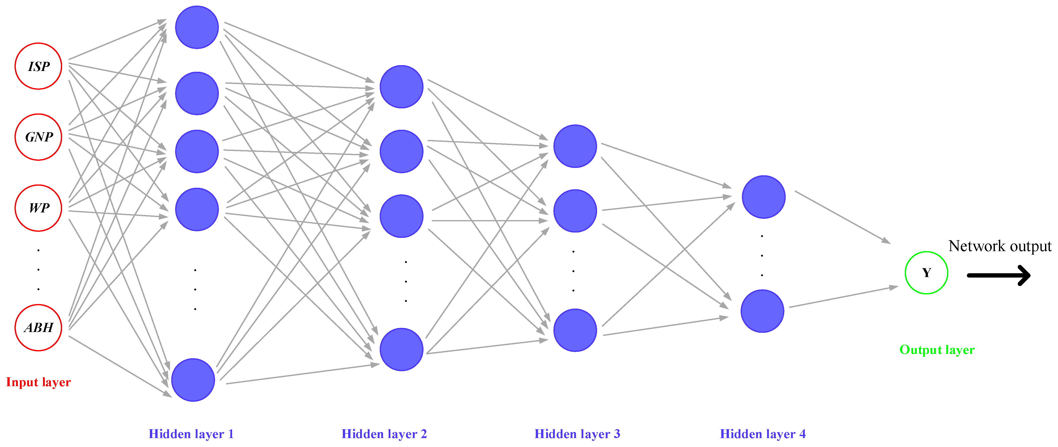
The urban planner adjusts the planning by regulating the control indexes of the blocks—on the one hand regulating the indexes of the land type to meet the urban land demand, and on the other hand regulating the scale of the buildings in the blocks by controlling the indexes of the building layout. Therefore, this study investigated the influence mechanism of morphological indexes on the thermal environment for the above controllable indexes. The block units were mainly expressed in two-dimensional space on different covers of the ground surface after zoning, and the ground cover indicators included the percentage of impervious surface (ISP), the percentage of green space (GNP), the percentage of water (WP), and the percentage of bare soil (BSP), which represented the type of land cover of the block units in the study area. In three dimensions, the distribution of buildings within a block unit was used to quantitatively describe the morphology [28]. Floor area ratio (FAR), building cover percentage (BCP), and average building height (ABH) were indicators used to characterize building patterns. In this study, land cover type and building group pattern, including seven morphological variables, were selected and used as indicators of block morphology. The details of the seven indexes are shown in

Table 1. Block morphological indexes.

Indexes	Description	Range of Values
Land cover
Impervious Surface Percentage (ISP)	Percentage of impervious surface in each block unit	0–100
Green Percentage (GNP)	Percentage of green area in each block unit	0–100
Water Percentage (WP)	Percentage of water area in each block unit	0–100
Bare Soil Percentage (BSP)	Percentage of bare soil land in each block unit	0–100
Building group
Floor Area Ratio (FAR)	Ratio of total floor area to building site area in each block unit	0–max
Building Cover Percentage (BCP)	Percentage of total buildings footprint area in each block unit	0–100
Average Building Height (ABH)	Average height of total buildings in each block unit	max

. The above data were calculated statistically using Arc GIS 10.6 based on the current land use status vector files provided by the MLIT of Japan.

This study used Landsat 8 OLI and TRIS data from May 2016 for LST inversions. The data used in this study were downloaded from “https://earthexplorer.usgs.gov/ (accessed on 2 December 2022)”. The data information is shown in

Table 2. Landsat 8 data information of study area.

LANDSAT_PRODUCT_ID	WRS_ROW	WRS_PATH	DATE_ ACQUIRED	CLOUD_COVER_ LAND
LC08_L1TP_112037_20160505_20200909_02_T1	37	112	2016-05-05	0.08
LC08_L1TP_113037_20160514_20200907_02_T1	37	113	2016-05-14	2.05

.

Firstly, Landsat 8 data were preprocessed, which included radiometric calibration and atmospheric correction (dark matter subtraction). It was necessary to convert the DN in the thermal band (B10 and B11) into absolute units of the sensor’s spectral radiance, in order to determine the study area’s LST. The digital number (DN) values were then transformed into satellite brightness temperature (TB) [29]. Secondly, the thermal band data were transformed from the spectral emissivity of the sensor to the effective brightness temperature of the sensor. The pre-launch calibration constant (specifically, the thermal conversion constants for Bands 10 or 11 provided in the Landsat-8 metadata used in this study) was used to perform the calculations [30]. This process was followed by a correction for spectral emissivity. The LST for emissivity correction was calculated as follows.

$$LST=\frac{T_B}{1+\left(\lambda \times T_B/\rho \right)\ln \epsilon }$$

(1)

where T_B is the brightness temperature of band 10 in Landsat 8; λ is the wavelength of the emitted radiation (the central wavelength of B10 is 10.8 μm); ρ = h × c/σ(1.438 × 10⁻² mk), where σ = Boltzmann constant (1.38 × 10⁻²³ J/K), h = Planck’s constant (6.626 × 10⁻³⁴ Js), and c = velocity of light (2.998 × 108 m/s); and ε is the land surface emissivity.

2.3. FNN Model

The feed-forward neural network (FNN) is a multilayer network trained according to the error back propagation (BP) algorithm. The algorithm uses the gradient descent method to determine the objective function’s minimum value, using the error square between the desired output value and the actual output value as the objective function [31]. As shown in a previous study [32], there is a relationship between a series of potential influences, such as morphological characteristics and urban heat island intensity, and the indicators show an interactive relationship. FNNs can map nonlinear relationships between independent and dependent variables, and can learn complex relationships between independent variables that affect each other.

We used Python to construct an FNN model containing an input layer, hidden layer, and output layer, and the structure is shown in Figure 5. This model contained one input layer, two hidden layers, and one output layer. The input layer was composed of seven morphological indicators of ISP, GNP, WP, BSP, FAR, BCP, and ABH for each block obtained in Section 2.1. Then, those input layers were weighted and transferred to the hidden layer. The output layer was the average LST data of the block units. In this FNN model, four hidden layers were set to avoid underfitting due to too few hidden layers. The number of neurons was generally 2ⁿ. Combining the number of implied layers, the first implied layer had 64 neurons, the second implied layer had 32 neurons, the third implied layer had 16 neurons, and the fourth implied layer had 8 neurons. To present the nonlinear relationship between input and output using the FNN, the hyperbolic tangent function (tanh) function was chosen as the activation function. The network’s learning rate was set to 0.001 and it was trained up to 100 times; the other parameters were left at their default values. Once convergence was reached, the FNN model was finished being built. The training was not finished until the network converged automatically, at which point the FNN model was created. The other parameters were set by default. First, the data were normalized; second, the dataset was split into training and testing sets to speed up network learning. The model used Adam as the optimizer and mean squared error (MSE) as the loss function. The expression of MSE is as follows:

$$MSE=\frac{1}{n}{{\displaystyle \sum _{i=1}^n\left(Y_i-{\widehat{Y}}_i\right)}}^2$$

(2)

where Y is the vector of observed values of the variable being predicted, and $\widehat{Y}$ represents the predicted values.

To date, a variety of neural network models have been established, among which the most widely used is the error backpropagation neural network, referred to as a fully connected neural network. Mean absolute error (MAE) represents the mean of the absolute error between the predicted and observed values. Root mean square error (RMSE) measures the deviation between the predicted and true values and is more sensitive to outliers in the data. The MAE and RMSE are calculated as follows:

$$MAE=\frac{1}{n}{\displaystyle \sum _{i=1}^n\left|{\widehat{y}}_i-y_i\right|}$$

(3)

$$RMSE=\sqrt{\frac{1}{m}{\displaystyle \sum _{i=1}^n{\left(y_i-{\widehat{y}}_i\right)}^2}}$$

(4)

where y is the vector of observed values of the variable being predicted, and $\widehat{y}$ represents the predicted values.

3. Results

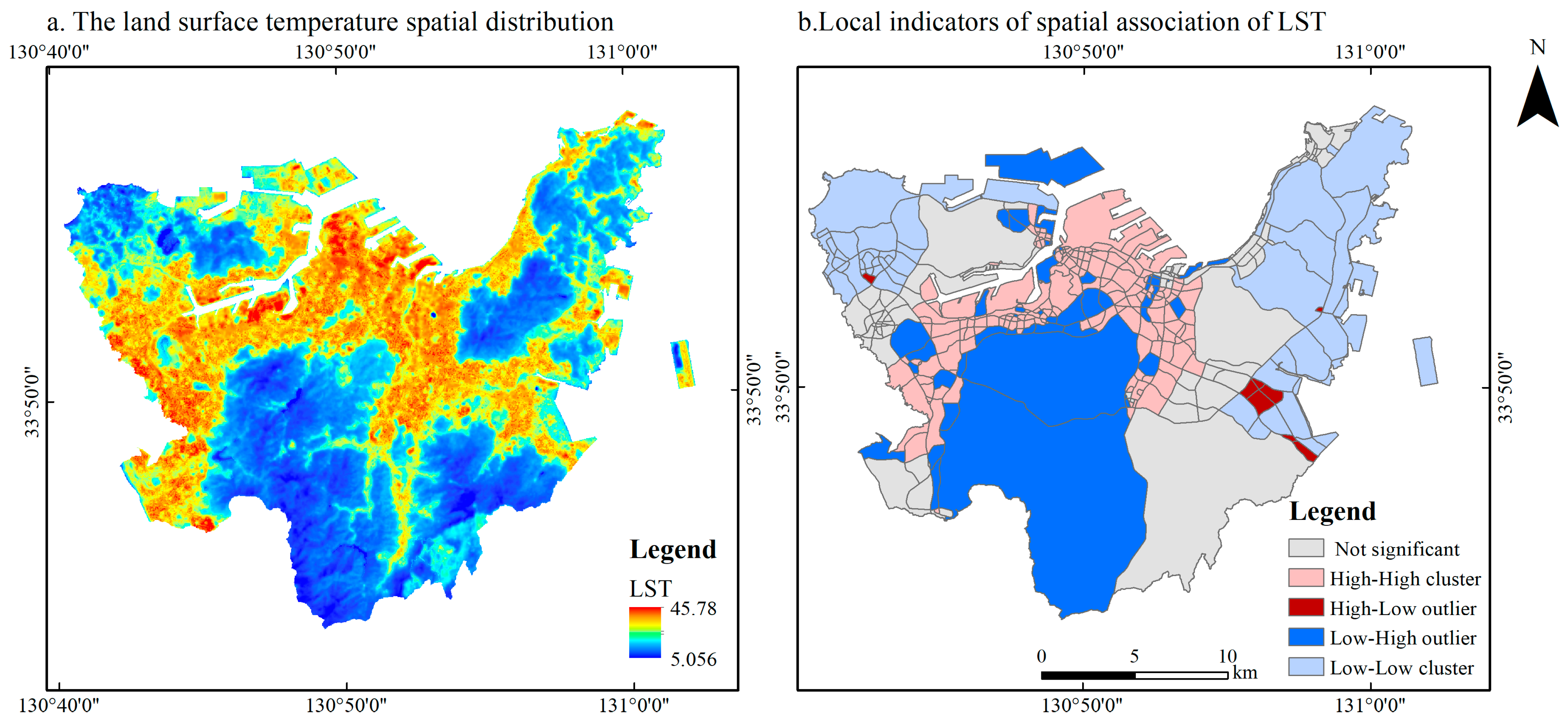
3.1. LST Spatial Distribution and Spatial Autocorrelation

Figure 6a shows the spatial distribution of the LST in Kitakyushu, which ranged from 5.06 to 45.78 °C during the daytime LST, with an average value of 19.083 °C. The average LST was 34.99 °C in the urban area and 26.25 °C in the suburbs, indicating a strong heat island effect in Kitakyushu. There were high central regions and lower north and south regions that made up Kitakyushu’s overall spatial distribution of LST, indicating that Kitakyushu is experiencing a severe urban heat island effect.

Global Moran’s I is a measure of the overall clustering of spatial data. The values range from −1 to 1. A value of 1 indicates complete positive spatial autocorrelation (high or low values clustered together), −1 indicates complete negative spatial autocorrelation (tessellation pattern), and 0 denotes complete spatial randomness [33]. The global Moran’s I index of LST in the study area was calculated, and Moran’s I was 0.181 (Zscore of 18.213; p-value of 0.000), indicating that the LST distribution in the study area appears to be spatially clustered.

The local Moran’s I index was used to further determine the relationship between the spatial distribution of aggregation categories and the functional distribution of block areas, and the results are shown in Figure 6b. The fact that Moran’s I is a summation of individual cross-products was exploited by the local indicators of spatial association (LISA) to evaluate the clustering in those individual units by calculating the local Moran’s I for each spatial unit and evaluating the statistical significance for each I_i [34], as follows:

$$I_{\mathrm{i}}=\frac{x_i-\overline{x}}{n}{\displaystyle \sum _{j=1}^N{\omega }_{ij}\left(x_j-\overline{x}\right)}$$

(5)

where n is the number of geographic units; x_i and x_j are the values at locations i and j, respectively; and ω_ij is the spatial weight matrix between locations i and j.

Thus, the LISA aggregation map of the LST identifies areas sensitive to heat island effects in order to optimize the targets of the block units. The pink areas in Figure 6b are high–high areas, and are mainly located in (1) the harbor logistics operation area and the industrial area along the south side of Donghae Bay, (2) the high-density urban mixed commercial and residential areas such as the Kokura Metropolitan Center and Kurosaki Vice Metropolitan Center, and (3) the densely populated areas around transportation hubs such as Yahata, Wakamatsu, Tobata, Jono, and Moritsune. The aggregation of low–low areas is mainly located in the area covered by mountain vegetation.

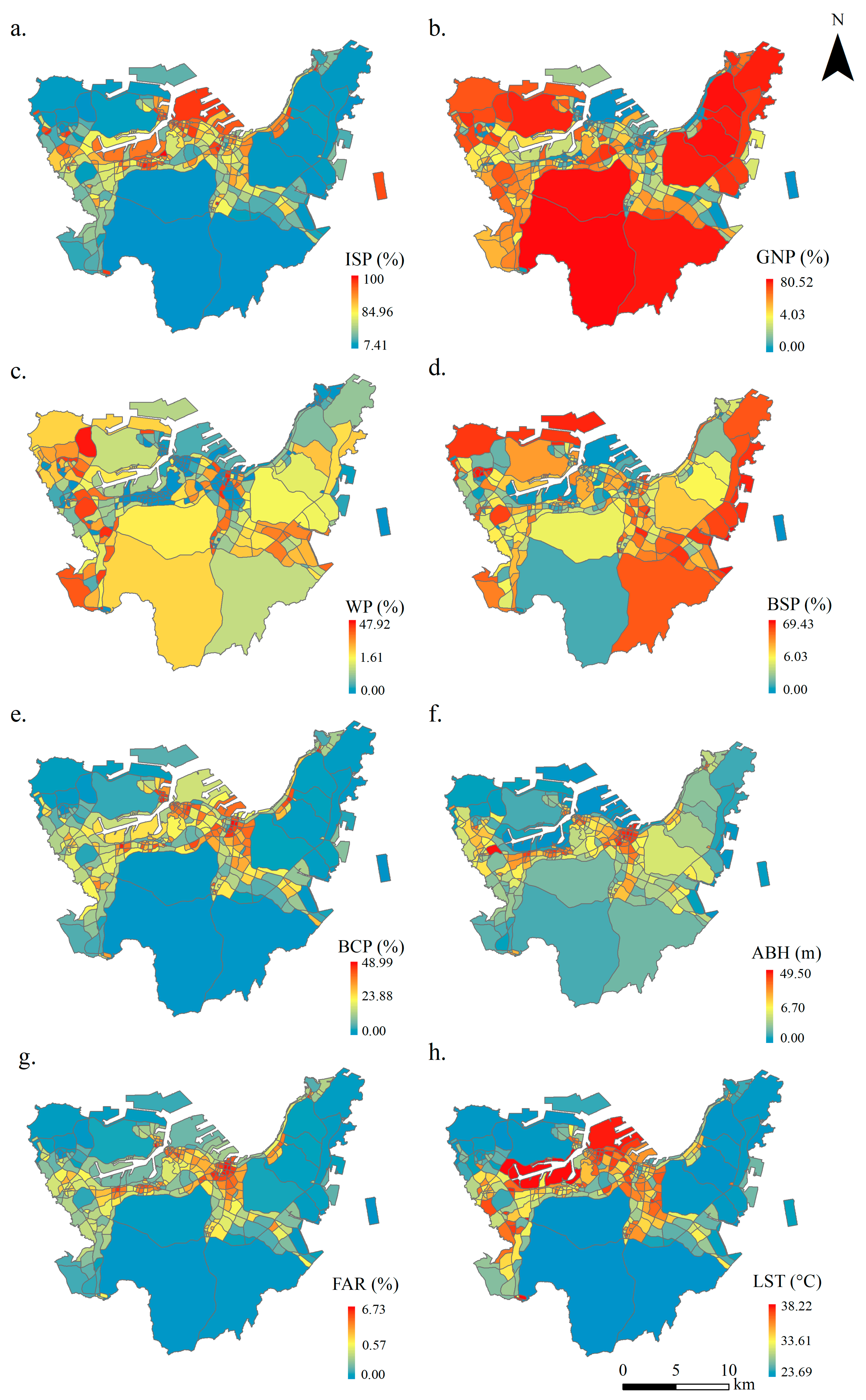
3.2. Distribution of Block Morphological Indexes

In this study, the indexes of each unit were calculated using Arc GIS based on the vector data of land use and building status in Kitakyushu provided by the MLIT, and the settlement results are shown in Figure 7. Figure 7a shows that the distribution of this indicator of ISP is higher in the built-up area because the north and south sides are mountainous; thus, the percentage of impervious surface is lower. As shown in Figure 7b, because the north and south sides of Kitakyushu are mountainous and forested, the GNP values in these two areas are also higher compared to the built-up areas. The water in Kitakyushu is mainly concentrated in the tributaries of the western Tonoga River and the forested area of the mountains, and there are few water bodies in the built-up area. It can be seen that the distribution of the WP indicators in Figure 7c is limited in the built-up area. The bare land in Kitakyushu is mainly undeveloped land and agricultural land, mostly located in the port operation area and unused vacant land in the suburban area (Figure 7d). The spatial distribution of land use indexes by block units shows that the ISP is higher in built-up areas and lower in GNP and BSP, mainly because after development and construction, the urban areas established with buildings, roads, squares, and other installations have become the main cover. The index factors of building morphology are shown in Figure 7e–g. From those figures, it can be seen that the areas with high values of each index are mainly concentrated in the areas with high population density in the Kokura Metropolitan Center and Kurosaki Subcenter.

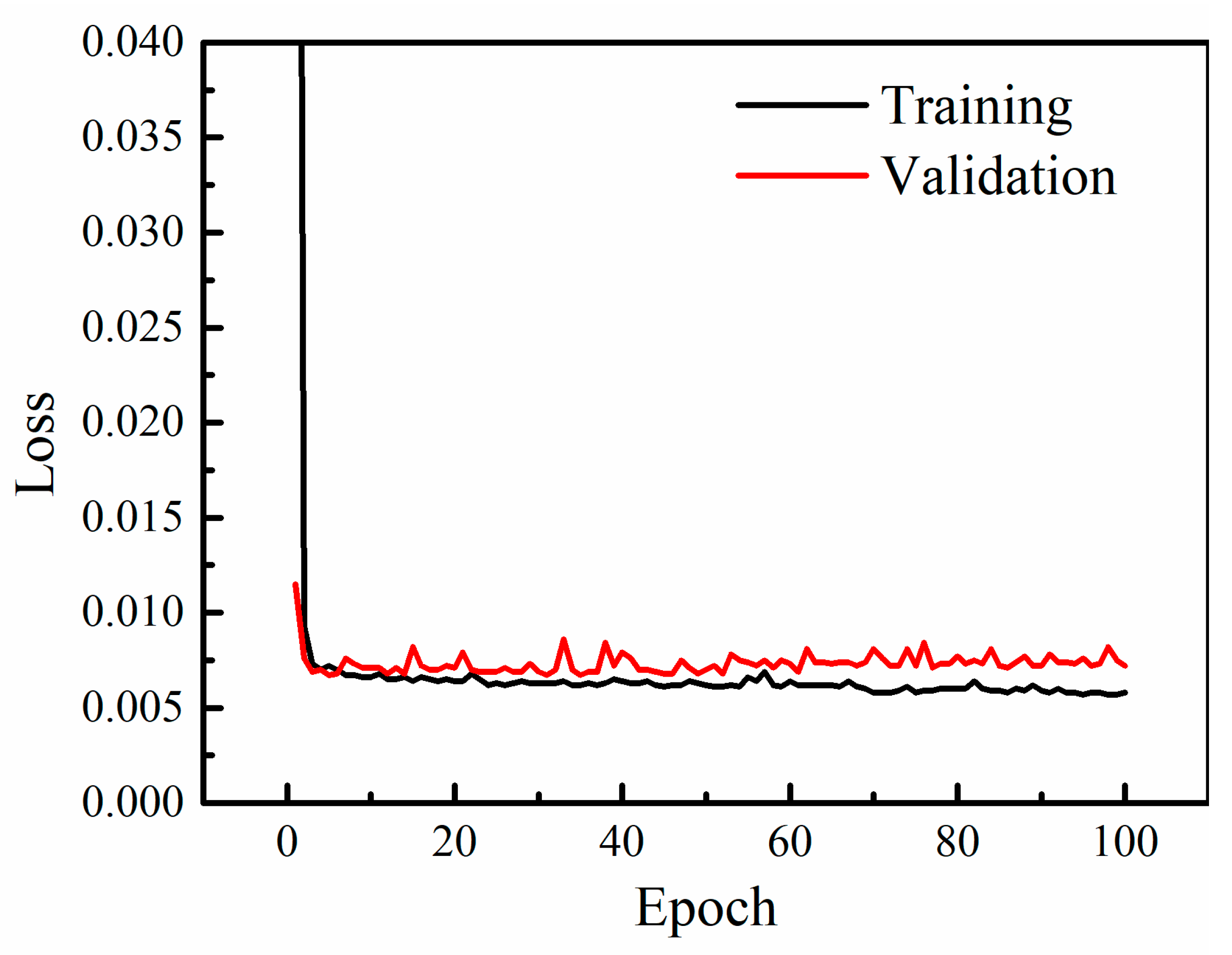
3.3. FNN Model Performance

The feed-forward neural network (FNN) model uses block morphological indicators and LST as input datasets for training. The FNN in this paper was based on Python and the TensorFlow deep learning framework. The neural network topology constructed in this study is a 7 × 64 × 32 × 16 × 8 × 1 neural network. Additionally, different FNN model settings were tested, and the FNN model with four hidden layers demonstrated the best accuracy and learning efficiency. After iterative learning and optimization in the network to find the intrinsic connection between each index and the LST, the model was used to analyze the relationship between the regional urban thermal environment and block morphology after the training was completed.

A proportion of 75% of the input data were used as the training set and 25% were used as validation for the FNN model. The dataset was split and selected in a random state. The training results are shown in Figure 8. It can be seen from Figure 8 that the model achieves convergence and minimum loss by 100 epochs. According to the loss decreasing curve, the training set converged faster and then decreased smoothly. The validation set converged and tended to converge to a stable state, and there was no significant increase in the loss value after decreasing during the training process. After 100 rounds of iterative training, the performance of the validation set became relatively stable with an MSE of 1.402, basically without significant fluctuations, and the model was stable and effective.

FNN is a black box model, aiming to reflect the hidden relationship between morphological indicators and LST. The study area’s built-up block indicators are connected to the LST by the FNN model. The results show that the experimental FNN model can reflect the complex and interactive relationship between morphological indicators and LST. According to the results, the hyperparameters of FNN enable the model to achieve an MSE of 1.402. The satisfactory precision achieved in this research can be used for LST prediction. The utility of the model consists of two main parts. On the one hand, it is possible to quantify the LST of a block or region by predicting the average LST from the input of seven morphological indicators. On the other hand, the combination of seven indicators can be optimized by adjusting seven indicators to achieve the optimization target with a regulation LST. In work on urban planning and renewal, the model can be used to regulate and optimize the indicators.

4. Discussion

4.1. Model Comparison

Ordinary least squares regression (OLS) and random forest (RF) were selected as the commonly used models for the regression of block morphological indicators and LST, and the accuracy of the three models was compared. OLS is a traditional statistical method for the quantitative analysis of relationships between dependent and independent variables [35,36]. The OLS model is a type of linear least squares method for choosing the unknown parameters in a linear regression model (with fixed level-one effects of a linear function of a set of explanatory variables) by the principle of least squares in the input dataset, and the output of the (linear) function of the independent variable. Random forest (RF) is similar a method more commonly used in machine learning to analyze nonlinear relationships between variables [37]. In recent years, it has also been used to evaluate the impact of various variables on LST [38,39]. The RF model is based on decision trees, each of which is built from randomly selected training samples and randomly selected predictor variables that are combined to generate the final predicted values. The number of weak classifiers (number of decision trees) in this model was 50, the maximum depth of the tree was set to 30, the measure of regression effectiveness was MSE, and the test and validation sets were randomly assigned 75% and 25% of the data, respectively. In this study, the LST was modeled with each morphological indicator using the OLS model, the RF model, and the FNN model. Then, the accuracy of the models was compared using performance metrics such as R², RMSE, and MAE, and the results are shown in

Table 3. Results of performance metrics.

Performance Metrics	OLS Model	RF Model	FNN Model
R2	0.730	0.657	0.781
RMSE	1.191	1.293	1.184
MAE	0.923	0.919	0.885

.

The results indicate that the FNN had a better fitting effect on the relationship between the morphological indicators and the LST. The results demonstrate that the R² value of the FNN model was higher than that of the OLS and RF models. The FNN model improved the fit by 6.1% over the OLS model. The RMSE and MAE results show that the FNN model had the highest accuracy for the prediction of LST. Overall, the FNN model better reflected the relationship between morphology indicators and LST.

4.2. Specific Application of Feed-Forward Neural Network Model

The validation and comparison results of the FNN model constructed in this study show that FNN can more effectively and accurately respond to the influence of morphological indicators on LST. Therefore, the results of the study have important implications for urban planning and design in the study area. We sought to predict LST of blocks by inputting the seven morphological indexes into the FNN model, and then quantitatively evaluating the blocks and regions based on predictive LST.

Therefore, a unit with a high LST was chosen to select indicators for adjustment. Ref. [38] pointed out that building density has a greater influence on changes in LST. It is difficult to change the building scale within already built-up areas. However, building density can be shaped by the design of the scheme stage for the areas that have not been planned yet. Ref. [16] pointed out that ISP and GNP have a strong influence on LST. Greater urban greenery significantly reduces temperatures [18,40] within a certain range. The cooling effect of green space is obvious, and obtaining the corresponding indexes of the ideal cooling effect of green space is key for the region’s planning [41]. Therefore, GNP was chosen as an example of an adjusted indicator to predict the LST distribution. It is worth noting that as GNP increased, the ISP decreased. According to the distribution of LST, the hotter block units were concentrated in the densely populated areas of the harbor industrial zone. In this study, a mixed residential and business block was selected; the real-world view is shown in Figure 9. Increasing the green space in the block unit by adding small public green space and optimizing the layout of parking lots would increase certain green space. The values of the seven morphological indexes of this unit are shown in

Table 4. Indicators of a typical unit.

Indicators	Value
Impervious Surface Percentage (ISP)	98.4% to 70%
Green Percentage (GNP)	1.6% to 30%
Water Percentage (WP)	0
Bare Soil Percentage (BSP)	0
Floor Area Ratio (FAR)	0.814
Building Cover Percentage (BCP)	32.2%
Average Building Height (ABH)	7.2 m

Maintaining the existing building scale, the bare surface and part of the impervious surface in the block are renewed as green space, and the indicators on the 2-dimensional aspect of the land cover are changed, but the total of the indicators is still 100%.

. The corresponding LSTs were calculated by the FNN model. The morphological indicators interact with each other. An increase in green space implies a decrease in impervious surfaces and bare ground. The ISP ranged from 98.4% to 70%, the GNP ranged from 1.6% to 30%, and the interval was set at 1%.

After inputting the seven indicators into the FNN model, a dot distribution map with the results of each combination was made and is displayed in Figure 10a. Numerous indicator scenarios are given in Figure 10a, but a single increase in green space will inevitably reduce impervious land. Therefore, the indicator scheme with the sum of GNP and ISP being 100% was selected, and the LST value predicted by the FNN model is shown in Figure 10b. With a difference of about 0.77 °C and a median of 33.58 °C, the LST determined by the model ranged from 33.19 °C to 33.96 °C. The lowest LST scenario was one in which the GNP fell to 30%, the ISP was simultaneously reduced to a 70% share, and the average LST of the block was 33.19 °C. It can be seen that when the ISP was constant, the LST gradually decreased as the GNP increased. Figure 10a shows that the area where the LST cooling effect was more pronounced in the index optimization scheme is the blue area above the black straight line at 33.58 °C. It can be seen that increasing the green space ratio can significantly reduce the thermal environment of the block. At the same time, it will also reduce the percentage of impervious surfaces, which to a certain extent will constrain construction and development. It is a suitable indicator for the block to increase the green space area as little as possible while achieving a certain cooling effect.

Many indicator scenarios are given in Figure 10a, but a single increase in green space will inevitably reduce impervious land. With the optimization target of cooling the LST to a median value of 33.58 °C, the specific indicator scheme was derived from the FNN model as GNP of 17.1%, ISP of 82.9%, WP of 0, BSP of 0, FAR of 0.814, BCP of 32.2%, and ABH of 7.2 m. Therefore, if the block is renewed, it can achieve a certain cooling effect while ensuring no development constraints on the building scale. The final suggested specific indicator scheme is based on the scale of current construction and development. With the LST serving as the control target, the method of this study was used to determine the specific combination of seven indicators for the area when carrying out urban renewal and urban planning work.

4.3. Limitations

Although this study used an artificial neural network to quantitatively explore the relationship between block morphology and LST, there are some limitations in this study. The main target of this study was to identify adjustable indicators in planning and design, in order to recommend strategies that can be used in urban planning and design based on the influence of certain indicators on LST. Climate also has an influence on the urban heat island phenomenon, but it cannot be adjusted through the deployment of planning and design indicators.

First, the non-smooth association between canopy climate and morphological factors should be considered comprehensively. Second, data from more sources should be introduced (e.g., meteorological monitoring data, 3D building information) for further determination of the strong correlation between individual morphological factors and LST. Lastly, Landsat 8 OLI and TRIS remote sensing images were the data sources for calculating the LST of the study area. The image resolution was 30 m, and this caused inaccuracies in the LST, especially for the small blocks. More interesting findings could be obtained and discussed based on higher-resolution images. More accurate remote sensing images and newer city morphological data should be updated in future studies.

5. Conclusions

Due to the numerous factors that affect its formation, growth, and evolution, the urban thermal environment is a complex system. A more accurate explanation of the relationship between morphological indicators and the complex interaction of land surface temperature (LST) can improve the prediction accuracy of LST. This study used a feed-forward neural network (FNN) model to examine the nonlinear relationship between morphological indicators and LST at the block scale. Seven morphological indicators and LST of Kitakyushu in Japan were collected and calculated by remote sensing and land cover data and used as the dataset for FNN model training. The constructed FNN model converged and reached the minimum loss at 100 epochs of training. Then, a strong heat island effect block with mixed commercial and residential functions was used as an example to clarify the specific application of the FNN model. Finally, with the LST serving as the control target, the method devised in this study was used to determine the optimal combination of seven indicators for the study area to guide urban renewal and urban planning work. The conclusions are as follows:

• The spatial autocorrelation of LST indicates that the areas sensitive to the heat island effect are mainly concentrated in the industrial area along the south side of Dong Bay, the high-density urban mixed commercial and residential areas, and densely populated areas around transportation hubs.
• The constructed FNN model converged and reached the minimum loss at 100 epochs of training. The R², RMSE, and MAE of the FNN model were 0.781, 1.184, and 0.885, respectively, showing better performance than ordinary least squares regression and random forest.
• Using cooling LST as the optimization target, the specific indicator scheme was derived from the FNN model with a GNP of 17.1%, ISP of 82.9%, WP of 0, BSP of 0, FAR of 0.814, BCP of 32.2%, and ABH of 7.2 m. With the LST serving as the control target, the method developed in this study was used to determine this specific combination of indicators for the area, which can inform urban renewal and urban planning work.

References

1. Stewart, I.D. A systematic review and scientific critique of methodology in modern urban heat island literature. Int. J. Climatol. 2011, 31, 200–217. [Google Scholar] [CrossRef]
2. Luber, G.; McGeehin, M. Climate Change and Extreme Heat Events. Am. J. Prev. Med. 2008, 35, 429–435. [Google Scholar] [CrossRef] [PubMed]
3. Ulpiani, G. On the linkage between urban heat island and urban pollution island: Three-decade literature review towards a conceptual framework. Sci. Total Environ. 2021, 751, 141727. [Google Scholar] [CrossRef]
4. Tan, J.; Zheng, Y.; Tang, X.; Guo, C.; Li, L.; Song, G.; Zhen, X.; Yuan, D.; Kalkstein, A.J.; Li, F.; et al. The urban heat island and its impact on heat waves and human health in Shanghai. Int. J. Biometeorol. 2010, 54, 75–84. [Google Scholar] [CrossRef]
5. Lu, Y.; Yue, W.; Huang, Y. Effects of Land Use on Land Surface Temperature: A Case Study of Wuhan, China. Int. J. Environ. Res. Public Health 2021, 18, 9987. [Google Scholar] [CrossRef] [PubMed]
6. Voogt, J.A.; Oke, T.R. Thermal remote sensing of urban climates. Remote Sens. Environ. 2003, 86, 370–384. [Google Scholar] [CrossRef]
7. Bechtel, B.; Demuzere, M.; Mills, G.; Zhan, W.; Sismanidis, P.; Small, C.; Voogt, J. SUHI analysis using Local Climate Zones—A comparison of 50 cities. Urban Clim. 2019, 28, 100451. [Google Scholar] [CrossRef]
8. Hu, Y.; Hou, M.; Jia, G.; Zhao, C.; Zhen, X.; Xu, Y. Comparison of surface and canopy urban heat islands within megacities of eastern China. ISPRS J. Photogramm. 2019, 156, 160–168. [Google Scholar] [CrossRef]
9. Estoque, R.C.; Murayama, Y.; Myint, S.W. Effects of landscape composition and pattern on land surface temperature: An urban heat island study in the megacities of Southeast Asia. Sci. Total Environ. 2017, 577, 349–359. [Google Scholar] [CrossRef]
10. Stewart, I.D.; Oke, T.R. Local Climate Zones for Urban Temperature Studies. Bull. Am. Meteorol. Soc. 2012, 93, 1879–1900. [Google Scholar] [CrossRef]
11. Kotharkar, R.; Bagade, A. Local Climate Zone classification for Indian cities: A case study of Nagpur. Urban Clim. 2018, 24, 369–392. [Google Scholar] [CrossRef]
12. Hu, J.; Ghamisi, P.; Zhu, X. Feature Extraction and Selection of Sentinel-1 Dual-Pol Data for Global-Scale Local Climate Zone Classification. ISPRS Int. J. Geo-Inf. 2018, 7, 379. [Google Scholar] [CrossRef] [Green Version]
13. Shareef, S.; Altan, H. Urban block configuration and the impact on energy consumption: A case study of sinuous morphology. Renew. Sustain. Energy Rev. 2022, 163, 112507. [Google Scholar] [CrossRef]
14. Berger, C.; Rosentreter, J.; Voltersen, M.; Baumgart, C.; Schmullius, C.; Hese, S. Spatio-temporal analysis of the relationship between 2D/3D urban site characteristics and land surface temperature. Remote Sens. Environ. 2017, 193, 225–243. [Google Scholar] [CrossRef]
15. Gao, Y.; Zhao, J.; Han, L. Exploring the spatial heterogeneity of urban heat island effect and its relationship to block morphology with the geographically weighted regression model. Sustain. Cities Soc. 2022, 76, 103431. [Google Scholar] [CrossRef]
16. Gao, Y.; Zhao, J.; Yu, K. Effects of block morphology on the surface thermal environment and the corresponding planning strategy using the geographically weighted regression model. Build. Environ. 2022, 216, 109037. [Google Scholar] [CrossRef]
17. Yang, C.; Zhu, W.; Sun, J.; Xu, X.; Wang, R.; Lu, Y.; Zhang, S.; Zhou, W. Assessing the effects of 2D/3D urban morphology on the 3D urban thermal environment by using multi-source remote sensing data and UAV measurements: A case study of the snow-climate city of Changchun, China. J. Clean. Prod. 2021, 321, 128956. [Google Scholar] [CrossRef]
18. Perini, K.; Magliocco, A. Effects of vegetation, urban density, building height, and atmospheric conditions on local temperatures and thermal comfort. Urban For. Urban Green. 2014, 13, 495–506. [Google Scholar] [CrossRef]
19. Wu, G.; Miao, Y.; Wang, F. Intelligent Design Model of Urban Landscape Space Based on Optimized BP Neural Network. J. Sens. 2022, 2022, 9704287. [Google Scholar] [CrossRef]
20. Deb, C.; Eang, L.S.; Yang, J.; Santamouris, M. Forecasting diurnal cooling energy load for institutional buildings using Artificial Neural Networks. Energy Build. 2016, 121, 284–297. [Google Scholar] [CrossRef]
21. Yeon-Hee Kim, J.B. Maximum Urban Heat Island Intensity in Seoul. J. Appl. Meteorol. Clim. 2001, 14, 651–659. [Google Scholar]
22. Ding, X.; Zhao, Y.; Fan, Y.; Li, Y.; Ge, J. Machine Learning-Assisted Mapping of City-Scale Air Temperature: Using Sparse Meteorological Data for Urban Climate Modeling and Adaptation; Research Square: Durham, NC, USA, 2023. [Google Scholar]
23. Almeida, C.M.; Gleriani, J.M.; Castejon, E.F.; Soares Filho, B.S. Using neural networks and cellular automata for modelling intra-urban land-use dynamics. Int. J. Geogr. Inf. Sci. 2008, 22, 943–963. [Google Scholar] [CrossRef]
24. Kuang, H. Prediction of Urban Scale Expansion Based on Genetic Algorithm Optimized Neural Network Model. J. Funct. Spaces 2022, 2022, 5407319. [Google Scholar] [CrossRef]
25. Liu, Y.; Zhu, Q.; Yao, D.; Xu, W. Forecasting Urban Air Quality via a Back-Propagation Neural Network and a Selection Sample Rule. Atmosphere 2015, 6, 891–907. [Google Scholar] [CrossRef] [Green Version]
26. Guan, Q.; Wang, L.; Clarke, K.C. An Artificial-Neural-Network-based, Constrained CA Model for Simulating Urban Growth. Cartogr. Geogr. Inf. Sci. 2005, 32, 369–380. [Google Scholar] [CrossRef] [Green Version]
27. Kawamoto, Y. Effect of Land-Use Change on the Urban Heat Island in the Fukuoka–Kitakyushu Metropolitan Area, Japan. Sustainability 2017, 9, 1521. [Google Scholar] [CrossRef] [Green Version]
28. Yin, C.; Yuan, M.; Lu, Y.; Huang, Y.; Liu, Y. Effects of urban form on the urban heat island effect based on spatial regression model. Sci. Total Environ. 2018, 634, 696–704. [Google Scholar] [CrossRef]
29. Simwanda, M.; Ranagalage, M.; Estoque, R.C.; Murayama, Y. Spatial Analysis of Surface Urban Heat Islands in Four Rapidly Growing African Cities. Remote Sens. 2019, 11, 1645. [Google Scholar] [CrossRef] [Green Version]
30. Survey, U.G. Product Guide: Provisional Landsat 8 Surface Reflectance Code (LASRC) Product; Department of Interior, US Geological Survey: Washington, DC, USA, 2016. [Google Scholar]
31. Ren, L.; An, F.; Su, M.; Liu, J. Exposure Assessment of Traffic-Related Air Pollution Based on CFD and BP Neural Network and Artificial Intelligence Prediction of Optimal Route in an Urban Area. Buildings 2022, 12, 1227. [Google Scholar] [CrossRef]
32. Lin, J.; Qiu, S.; Tan, X.; Zhuang, Y. Measuring the relationship between morphological spatial pattern of green space and urban heat island using machine learning methods. Build. Environ. 2023, 228, 109910. [Google Scholar] [CrossRef]
33. Fu, W.J.; Jiang, P.K.; Zhou, G.M.; Zhao, K.L. Using Moran’s I and GIS to study the spatial pattern of forest litter carbon density in a subtropical region of southeastern China. Biogeosciences 2014, 11, 2401–2409. [Google Scholar] [CrossRef]
34. Anselin, L. Local Indicators of Spatial Association-LISA. Geogr. Anal. 1995, 27, 93–115. [Google Scholar] [CrossRef]
35. Li, L.; Zha, Y.; Zhang, J. Spatially non-stationary effect of underlying driving factors on surface urban heat islands in global major cities. Int. J. Appl. Earth Obs. 2020, 90, 102131. [Google Scholar] [CrossRef]
36. Guo, A.; Yang, J.; Sun, W.; Xiao, X.; Xia Cecilia, J.; Jin, C.; Li, X. Impact of urban morphology and landscape characteristics on spatiotemporal heterogeneity of land surface temperature. Sustain. Cities Soc. 2020, 63, 102443. [Google Scholar] [CrossRef]
37. Breiman, L. Random Forests. Mach. Learn. 2001, 45, 5–32. [Google Scholar] [CrossRef] [Green Version]
38. Wang, Q.; Wang, X.; Zhou, Y.; Liu, D.; Wang, H. The dominant factors and influence of urban characteristics on land surface temperature using random forest algorithm. Sustain. Cities Soc. 2022, 79, 103722. [Google Scholar] [CrossRef]
39. Wu, Q.; Li, Z.; Yang, C.; Li, H.; Gong, L.; Guo, F. On the Scale Effect of Relationship Identification between Land Surface Temperature and 3D Landscape Pattern: The Application of Random Forest. Remote Sens. 2022, 14, 279. [Google Scholar] [CrossRef]
40. Sodoudi, S.; Zhang, H.; Chi, X.; Müller, F.; Li, H. The influence of spatial configuration of green areas on microclimate and thermal comfort. Urban For. Urban Green. 2018, 34, 85–96. [Google Scholar] [CrossRef]
41. Zhang, Q.; Zhou, D.; Xu, D.; Rogora, A. Correlation between cooling effect of green space and surrounding urban spatial form: Evidence from 36 urban green spaces. Build. Environ. 2022, 222, 109375. [Google Scholar] [CrossRef]
Figure 1. The flow chart of study.
Buildings 13 00528 g001
Figure 2. Location of the study area.
Buildings 13 00528 g002
Figure 3. Monthly temperature distribution of Kitakyushu in the past 30 years (data from Japan Meteorological Agency).
Buildings 13 00528 g003
Figure 4. Units of the study area.
Buildings 13 00528 g004
Figure 5. FNN model structure of the study.
Buildings 13 00528 g005
Figure 6. Land surface temperature spatial distribution of study area. (a) LST distribution, (b) LISA aggregation map.
Buildings 13 00528 g006
Figure 7. Block index spatial distribution of study area: (a) ISP; (b) GNP; (c) WP; (d) BSP; (e) BCP; (f) ABH; (g) FAR; (h) LST.
Buildings 13 00528 g007
Figure 8. Loss curve of FNN model.
Buildings 13 00528 g008
Figure 9. Realistic picture of a typical unit.
Buildings 13 00528 g009
Figure 10. Distribution of predictive LST based on the FNN model: (a) LST matrices, (b) LST with GNP + ISP = 100%.
Buildings 13 00528 g010