Evaluating the Reactions of Bridge Foundations to Combined Wave–Flow Dynamics

Abstract

As the ongoing development of national infrastructure progresses, we see an increase in the construction of deep-water bridges, specifically cross-sea bridges. This paper uses Stokes’s wave theory to simulate and analyze how a bridge foundation dynamically responds to wave–fluid interactions. Firstly, the governing equations, boundary conditions and initial conditions of fluid motion are derived, expanded and solved via Stokes’s wave theory, and a spectral model is simulated and plotted. Based on the P-M spectrum and equal frequency method, a method of wave height attenuation during wave propagation is proposed. Using an SSTK-ω turbulence model, a numerical wave flume is established considering the fluid model, the selection of element type and the boundary conditions set, and the influencing factors of wave propagation (attenuation) are analyzed. Waves with different wave parameters (period, depth and height) are numerically simulated and compared with the theoretical values. Finally, we perform an analysis of the dynamic response under wave–current coupling conditions. We establish different operational scenarios and obtain the following results: under a load duration of 200 s, the peak transverse displacements for spans 1, 2 and 3 measure at 0.84 m, 0.63 m and 0.62 m, respectively. The peak transverse displacements under operational scenarios 2 and 3 show reductions of 25.0% and 25.7%, respectively, when compared to scenario 1. However, large transverse displacements remain. This suggests that the influence of waves and water flow on the transverse displacement of the main span should not be overlooked.

1. Introduction

Since the beginning of the 21st century, the global economy has been developing rapidly; at the same time, major economies have urgently sought to improve the construction of infrastructure in order to enhance cross-regional connectivity and develop new economic growth engines, and all major economies have made the construction of a strong transportation network their primary development goal [1]. With the solid progress of China’s “Belt and Road” strategy, a series of coordinated regional development strategies, such as the “Guangdong-Hong Kong-Macao Greater Bay Area” strategy, have been steadily implemented. The increasing demand for land transportation and economic development in China’s coastal and western areas has prompted the construction of bridges in China to enter a stage of rapid development [2]. Unlike land bridges, deep-water bridges are built in complex environments such as rivers, reservoirs and oceans and face more complex and variable hydrodynamic environments. As a link in the national transportation artery, once the main structure of a deep-water bridge loses some or all of its load-bearing capacity, it retards or blocks the transportation network, causing a serious public crisis in turn [3]. In the complex hydrodynamic environment, deep-water bridges are inevitably subjected to complex hydrodynamic effects such as waves and currents, especially under the effects of extreme sea conditions, which are highly likely to cause bridge damage or even collapse due to the strong impact of waves.

Currently, Lieberherr, E. et al. suggest that the association of multiple actors may have a number of effects, such as the redistribution of power among actors, changes in democratic control and the influence of citizens and changes in accountability structures [4]. Based on the nonlinear Morison equation, Wu A. J. et al. mounted structural dynamics equations underneath the blended motion of waves, currents and earthquakes and calculated the dynamic response of a deep-water pile-bearing abutment–bridge–pier structural device via finite aspect discretization, analyzing the effects of extraordinary wave glide factors on the dynamic response of this structural device [5]. Mondal, M. S., carried out a nationwide evaluation of nearby scour on the complicated piers of 239 bridges in Bangladesh, with 239 subject visits, 1434 km of bathymetric surveys and a tremendous amount of 478 mattress soil samples amassed and analyzed [6]. Tan Zhuang et al. established a fluid–solid coupling finite element model for the entire process of bridge construction, analyzed the influences of different flow velocities and water depths on the resistance and lateral force of pile-group-foundation piers and studied the flow field around the piers and the development of the law of flow stress with time under the flood discharge state [7]. Abdelhaleem, F. S., et al. investigated the pressure flow scour depth below exploratory clear water experiments in the presence of two vertical wall sills beside the bridge deck, and two assessments were performed involving the incoming waft depth, mattress cloth dimensions, shrinkage length and width and the prerequisites of bridge opening due to stress and free floor drift [8].

In this paper, the dynamic response of a bridge foundation to wave–flow coupling is simulated and analyzed using Stokes’s wave theory and an SSTK-ω turbulence model. A dynamic analysis of the response to wave–current coupling was carried out. Different working conditions were set up, and it was found that the effects of waves and currents on transverse displacement in the main span could not be neglected.

2. Stokes’s Wave Theory and Its Wave–Flow Coupling Action Theory

2.1. Control Equations and Boundary Conditions for Fluid Motion

The water wave theory uses the laws of fluid mechanics to reveal the essence of water wave motion, which requires the establishment of basic control equations suitable for fluid motion. The layout plan of a bridge is shown in Figure 1. In this paper, for gravity waves, the fluid is assumed to be incompressible, of constant density and non-viscous [9].

Let the mass in the flow field with density $\rho$ and volume of fluid V be

$$M(t)={\displaystyle {\displaystyle \underset{V(t)}{\iiint }}\rho dV,}$$

(1)

According to the law of conservation of mass, the following can be obtained:

$$\frac{dM}{dt}=0,$$

(2)

By deriving Equation (1), we obtain the following:

$$\frac{D\rho }{Dt}+\rho \nabla \cdot u=0,$$

(3)

where u is the fluid velocity in space (x, y, z) at the moment t. Since the fluid has been assumed to be incompressible, we have the following:

$$\frac{D\rho }{Dt}=0,$$

(4)

This leads to the following:

$$\nabla \cdot u=0,$$

(5)

If spinless flow is assumed, then we have the following:

$$\nabla \times u=0,$$

(6)

Then, there exists a velocity potential Φ. Substituting this into Equation (5), we obtain the following:

$${\nabla }^2\Phi =0,$$

(7)

The above equation is the Laplace equation of fluid motion, which is the basic kinematic equation governing the fluid [10]. Newton’s second law is applied to the fluid to obtain the following:

$$\frac{d}{dt}{\displaystyle {\displaystyle \underset{V}{\iiint }}\rho udV}={\displaystyle {\displaystyle \underset{V}{\iiint }}FdV}-{\displaystyle \underset{S}{{\displaystyle \iint }}}pndS,$$

(8)

Thus, the momentum equation can be obtained as follows:

$$\frac{\partial u}{\partial t}+(u\cdot \nabla )u=-\nabla \left(gz+\frac{p}{\rho }\right),$$

(9)

The Bernoulli integration of the spatial coordinates for Equation (9) yields the following:

$$\mathsf{\Phi }+\frac{1}{2}|\nabla \mathsf{\Phi }{|}^2+\frac{p}{\rho }+gz=f(t),$$

(10)

$$\mathsf{\Phi }+\frac{1}{2}|\nabla \mathsf{\Phi }{|}^2+\frac{p}{\rho }+gz=\frac{p_a}{\rho },$$

(11)

In summary, the continuity Equation (5) and the momentum Equation (9) can be replaced by the Laplace Equation (7) and the Bernoulli equation integral (10), respectively, under the assumptions of spinelessness and incompressibility [11]. However, the momentum Equation (9) contains a set of nonlinear differential equations with multiple unknowns for which analytical solutions exist only in very special cases and are complex to solve numerically [12]. In contrast, the Laplace Equation (7) is a linear partial differential equation with only one unknown quantity which has a theoretically sound and methodologically mature solution.

From the wave-free surface condition, the vertical velocity of the mass is as follows:

$$\frac{dz}{dt}=\frac{\partial \eta }{\partial t}+\frac{\partial \eta }{\partial x}\frac{\partial x}{\partial t}+\frac{\partial \eta }{\partial y}\frac{\partial y}{\partial t},$$

(12)

where x, y and z are the spatial scales of the fluid mass; thus, the velocity of the motion of the mass is

$$\left(\frac{\partial x}{\partial t},\frac{\partial y}{\partial t},\frac{\partial z}{\partial t}\right)=(u,v,w)=\left(\frac{\partial \mathsf{\Phi }}{\partial x},\frac{\partial \mathsf{\Phi }}{\partial y},\frac{\partial \mathsf{\Phi }}{\partial z}\right),$$

(13)

where u, v and w are the velocity components of the fluid mass, which can be obtained from the above two equations.

$$\frac{\partial \eta }{\partial t}+\nabla \mathsf{\Phi }\cdot \nabla \eta =\frac{\partial \mathsf{\Phi }}{\partial x},z=\eta (x,y,t),$$

(14)

Since the pressure on the free surface is equal to the atmospheric pressure above, its substitution into Equation (11) yields the following:

$$\frac{\partial \mathsf{\Phi }}{\partial t}+\frac{1}{2}\left(|\nabla \mathsf{\Phi }{|}^2+{\left(\frac{\partial \mathsf{\Phi }}{\partial z}\right)}^2\right)+g\eta =0,$$

(15)

Using Equations (14) and (15) to eliminate η, we obtain the free surface condition expressed by Φ, which combines the kinematic and kinetic conditions.

$$\frac{{\partial }^2\mathsf{\Phi }}{\partial t^2}+g\frac{\partial \mathsf{\Phi }}{\partial z}+2\nabla \mathsf{\Phi }\cdot \nabla \frac{\partial \mathsf{\Phi }}{\partial t}+\frac{1}{2}\nabla \mathsf{\Phi }\cdot \nabla (\nabla \mathsf{\Phi }\cdot \nabla \mathsf{\Phi })=0,$$

(16)

The unit normal vector of the underwater surface is

$$n=\left(n_x,n_y,n_z\right)=\frac{\left(F_x,F_y,F_z\right)}{\sqrt{F_x^2+F_y^2+F_z^2}}=\frac{\left(h_x+h_y+1\right)}{\sqrt{h_x^2+h_y^2+1}},$$

(17)

Then the normal velocity of the water’s bottom surface is

$$h_t{n}_z=\frac{h_t}{\sqrt{F_x^2+F_y^2+F_z^2}},$$

(18)

Then the normal velocity of the fluid mass at the bottom of the water is

$$\nabla \mathsf{\Phi }\cdot n=\frac{\left(F_x{\mathsf{\Phi }}_x,F_y{\mathsf{\Phi }}_y,F_z{\mathsf{\Phi }}_z\right)}{\sqrt{F_x^2+F_y^2+F_z^2}}=\frac{\left(h_x{\mathsf{\Phi }}_x+h_y{\mathsf{\Phi }}_y+{\mathsf{\Phi }}_z\right)}{\sqrt{h_x^2+h_y^2+1}},$$

(19)

Neglecting the permeability of the water bottom, the normal velocity of the surface underwater is the same as that of the mass point on it [13]. Thus, we have the following:

$$\frac{\partial h}{\partial t}+\frac{\partial h}{\partial x}\frac{\partial \mathsf{\Phi }}{\partial x}+\frac{\partial h}{\partial y}\frac{\partial \mathsf{\Phi }}{\partial y}+\frac{\partial \mathsf{\Phi }}{\partial z}=0,$$

(20)

If the underwater surface is assumed to not change with time, then

$$\frac{\partial h}{\partial x}\frac{\partial \mathsf{\Phi }}{\partial x}+\frac{\partial h}{\partial y}\frac{\partial \mathsf{\Phi }}{\partial y}+\frac{\partial \mathsf{\Phi }}{\partial z}=0or-\nabla h\cdot \nabla \mathsf{\Phi }=\frac{\partial \mathsf{\Phi }}{\partial z},$$

(21)

From the preliminary prerequisites of wave motion, shown in Equation (7), the manipulation of the equation of wave motion includes partial derivatives with respect to the spatial coordinates and partial derivatives with respect to time; therefore, the solution to the manipulation of the equation requires not only the preliminary values of the movement variables in space but also the preliminary values of the action variables, i.e., the preliminary prerequisites [14]. To ensure the strength of the solution, preliminary stipulations are assumed as follows:

$${\left.\Phi \right|}_{t=0}=f_1(x,y)z=\eta (x,y,0),$$

(22)

$${\left.\frac{\partial \Phi }{\partial t}\right|}_{t=0}=f_2(x,y)z=\eta (x,y,0),$$

(23)

2.2. Stokes’s Wave Theory

The velocity potential and wavefront elevation of the second-order theory of Stokes’s waves can be expressed as follows:

$$\begin{array}{l}\mathsf{\Phi }={\mathsf{\Phi }}^{(1)}+{\mathsf{\Phi }}^{(2)}=\frac{Aw}{k}\left[\frac{chk(z+h)}{shkh}\sin \theta +\frac{3}{8}Ak\frac{ch2k(z+h)}{s{h}^{4}kh}\sin 2\theta \right]\\ \eta ={\eta }^{(1)}+{\eta }^{(2)}=A\left[-\frac{Ak}{2sh2kh}\cos \theta +\frac{Ak}{4}\frac{chkh\left(2c{h}^{2}kh+1\right)}{s{h}^{3}kh}\cos 2\theta \right]\end{array},$$

(24)

where θ = kx − wt. As the wave steepness ε = A/L becomes larger, the contributions of the second-order quantities become appreciable. Figure 2 provides the first-order quantity wavefront elevation η, second-order quantity wavefront elevation η and Stokes’s second-order wavefront elevation η when Ak = 0.4.

By taking partial derivatives of Equation (24), the horizontal u and vertical components w of the velocity at the water quality point can be obtained.

$$u=\frac{\partial \mathsf{\Phi }}{\partial x}=Aw\left[\frac{chk(z+h)}{shkh}\cos \theta +\frac{3}{4}Ak\frac{ch2k(z+h)}{s{h}^{4}kh}\cos 2\theta \right],$$

(25a)

$$v=\frac{\partial \mathsf{\Phi }}{\partial z}=Aw\left[\frac{shk(z+h)}{shkh}\sin \theta +\frac{3}{4}Ak\frac{sh2k((z+h)}{s{h}^{4}kh}\sin 2\theta \right],$$

(25b)

From the above two equations, it can be seen that the water quality point velocity of the horizontal u and the straight component w curve and the 2 surface elevation curve shown in Figure 2 are similar, that is, there is an upper asymmetry and a lower asymmetry, and the asymmetry is an important nonlinear characteristic of the study of coastal sediment movement. Then, the horizontal acceleration of the water quality point is as follows:

$$a_x=\frac{\partial u}{\partial t}=2\left(\frac{{\pi }^{2}H}{T^2}\right)\frac{chkz}{shkh}\sin (kx-wt)+3\left(\frac{{\pi }^{2}H}{T^2}\right)\left(\frac{\pi H}{L}\right)\frac{sh2kz}{s{h}^{4}kh}\sin 2(kx-wt),$$

(26)

The vertical acceleration of the water mass point is as follows:

$$a_z=\frac{\partial v}{\partial t}=-2\frac{H{\pi }^2}{T^2}\frac{shkz}{shkh}\cos (kx-wt)-3\left(\frac{{\pi }^{2}H}{T^2}\right)\left(\frac{\pi H}{L}\right)\frac{sh2kz}{s{h}^{4}kh}\cos 2(kx-wt),$$

(27)

From the equation, can be seen that the horizontal velocity exists as a constant component, that is, the first term at the right end of the first equation above [15]. The result of this constant velocity is that the trajectory of the water quality point is not enclosed; the water quality point will be driven forward with the wave, and the constant component is called the mass transport velocity <u>.

$$〈u〉=\frac{c}{2}{(Ak)}^2\frac{ch2k\left(z_0+h\right)}{s{h}^{2}kh},$$

(28)

The flow rate Q along the water depth section can then be obtained as follows:

$$Q={\displaystyle \underset{-h}{\overset{0}{{\displaystyle \int }}}}〈u〉d{z}_0=\frac{c}{4k}{(Ak)}^2\frac{sh2kh}{s{h}^{2}kh}=\frac{E}{\rho c},$$

(29)

2.3. Theory of Wave–Current Coupling Action

When the joint action of wave and water flow is assumed, we have the following:

(1)

The surface of the pile column is smooth.

(2)

The hydrodynamic coefficient is constant along the water depth when the wave and current coexist.

(3)

In the wave flow field, Stokes’s wave theory is used to calculate the velocity and acceleration at the water quality point.

(4)

When the wave and flow coexist, the velocity and acceleration of the water quality point for the wave and the water flow are generated by the respective velocity and acceleration vectors.

At this time, the wave flow field velocity potential can be written as

$${\varphi }^{\prime }=Ux+\varphi ,$$

(30)

The kinematic boundary conditions after linearization are

$$\frac{\partial \eta }{\partial t}+\frac{\partial \eta }{\partial x}U-\frac{\partial \varphi }{\partial z}=0z=0,$$

(31)

The dynamic boundary condition of the free water surface is

$$\frac{\partial {\varphi }^{\prime }}{\partial t}+\frac{1}{2}\left[{\left(\frac{\partial {\varphi }^{\prime }}{\partial x}\right)}^2+{\left(\frac{\partial {\varphi }^{\prime }}{\partial z}\right)}^2\right]+g\eta =f(t)z=0,$$

(32)

The second order term is omitted to obtain

$$\frac{\partial \varphi }{\partial t}+U\frac{\partial \varphi }{\partial x}+\frac{1}{2}{U}^2+g\eta =f(t)z=0,$$

(33)

There is only water without waves in the infinite distance, so the above equation can be written as

$$\frac{\partial \varphi }{\partial t}+U\frac{\partial \varphi }{\partial x}+g\eta =0z=0,$$

(34)

The conjunction (31)–(34) yields

$${\left(\frac{\partial }{\partial t}+\frac{\partial }{\partial x}U\right)}^2\varphi +g\frac{\partial \varphi }{\partial z}=0z=0,$$

(35)

The velocity potential and wavefront can be written as

$$\varphi =\frac{A\cosh k(z+d)}{\cosh kd}\sin (kx-\omega t),$$

(36)

$$\eta =H\cos (kx-\omega t),$$

(37)

Substituting Equations (36) and (37) into (31) yields

$$\varphi =\frac{Hg\cosh k(z+d)}{{\omega }^{\prime }\cosh kd}\sin (kx-\omega t),$$

(38)

$${\omega }^{\prime }=\omega -kU={(gkthkh)}^{1/2},$$

(39)

The velocity potential under wave–flow coexistence can be obtained from Equation (30) [16].

$${\varphi }^{\prime }=Ux+\frac{Hg\cosh k(z+d)}{{\omega }^{\prime }\cosh kd}\sin (kx-\omega t),$$

(40)

The velocity of the water mass under wave coexistence is

$$u=\frac{\partial {\varphi }^{\prime }}{\partial x}=U+\frac{Hgk\cosh k(z+d)}{{\omega }^{\prime }\cosh kd}\cos (kx-\omega t),$$

(41)

$$w=\frac{\partial {\varphi }^{\prime }}{\partial z}=\frac{Hgk\sinh k(z+d)}{{\omega }^{\prime }\cosh kd}\sin (kx-\omega t),$$

(42)

The wave velocities in the absence of current are c₀ and L₀.

$$L_0=\frac{2\pi c_0^2}{gth{k}_{0}h},$$

(43)

The wave velocity in the presence of water flow is c, and the wavelength is L. They are obtained from [17] as follows:

$$c=\frac{{(gkthkh)}^{1/2}}{k},$$

(44)

$$L=\frac{2\pi c^2}{gthkh},$$

(45)

It is assumed that the wave frequency and wave frequency do not change i.e.,

$$\frac{L_0}{c_0}=\frac{L}{c+U},$$

(46)

3. Numerical Modeling of Bridge Foundations under Wave–Flow Coupling

3.1. Sink Simulation of Wave Flow

The selected wave parameters are wave height: 5.0 m; period: 7.0 s; and water depth: 20 m. From Stokes’s second-order wave theory, the wave wavelength is 71.9821 m, the wave frequency is w = 2/T = 0.8976, and the wave number is k = 2/L = 0.0873. To accurately reflect the simulation of waves in the water tank, the length of the water tank is taken to be six wavelengths, and the width is taken as 15 m. The riverbed cross-section is shown in Figure 3.

According to the theory of a linear wave-generating plate, the velocity function of the wave-generating plate at the wave inlet can be calculated. To avoid the influence of wave reflection on wave height, the calculation time is cut off before the wave reaches the right boundary and begins to reflect, that is, at six wave cycles [18].

An incompressible viscous flow is used in the water column to simulate the water more realistically, and an eight-node hexahedral FCBI-C cell is used to simulate the fluid [19]. The fluid parameters are as follows: river density, ρ_w = 1025 kg/m³; hydrodynamic viscosity coefficient, u = 1.01 × 10⁻³ kg/(m·s); and gravitational acceleration, g = 9.8 N/m².

For the 3D numerical wave flume, the corresponding boundary conditions must be set for the six boundaries of the 3D computational domain. The boundary conditions of the flume are as follows: the bottom and side boundaries use slidable solid-wall boundaries, the upper surface uses a free liquid surface boundary, and the wave outlet (right boundary) uses a consistent flow boundary [20]. From the two-dimensional perspective of the wave surface effect, it can be seen that the created waves have alternating crests and troughs which can simulate a more ideal regular wave. However, the simulated waves do not reach the set wave height of 5.0 m, as can be seen from the fluctuation in the elevation of the free liquid surface. From the three-dimensional view, it can be seen that the wave decays quickly after a certain distance from the wave inlet, and the wave at the near outlet has completely decayed. The attenuation of wave height in the direction of wave propagation is a common problem in numerical wave simulation, and the following will analyze the process of setting wave propagation to minimize the attenuation of wave height during wave propagation.

In order to further observe the attenuation of wave height in the wave simulation, the “Model Point” is defined at 0, 0.5 L, L and 2 L (in which L is the wavelength) from the incident boundary on the free liquid surface, and the time course curve of the wave displacement is obtained at the corresponding points. Figure 4 shows the fluctuation displacement time curve of each point. From the figure, it can be considered that the farther away from the wave source, the sparser the grid division becomes in the course of wave propagation, and the attenuation of the wave peaks at the free floor points becomes particularly apparent. It can be considered that the degree of wave peak attenuation is extensively associated with the measurement of the grid density in the course of wave propagation (i.e., the x-direction of this model).

3.2. Numerical Simulation of Wave Flow under Different Wave Flow Parameters

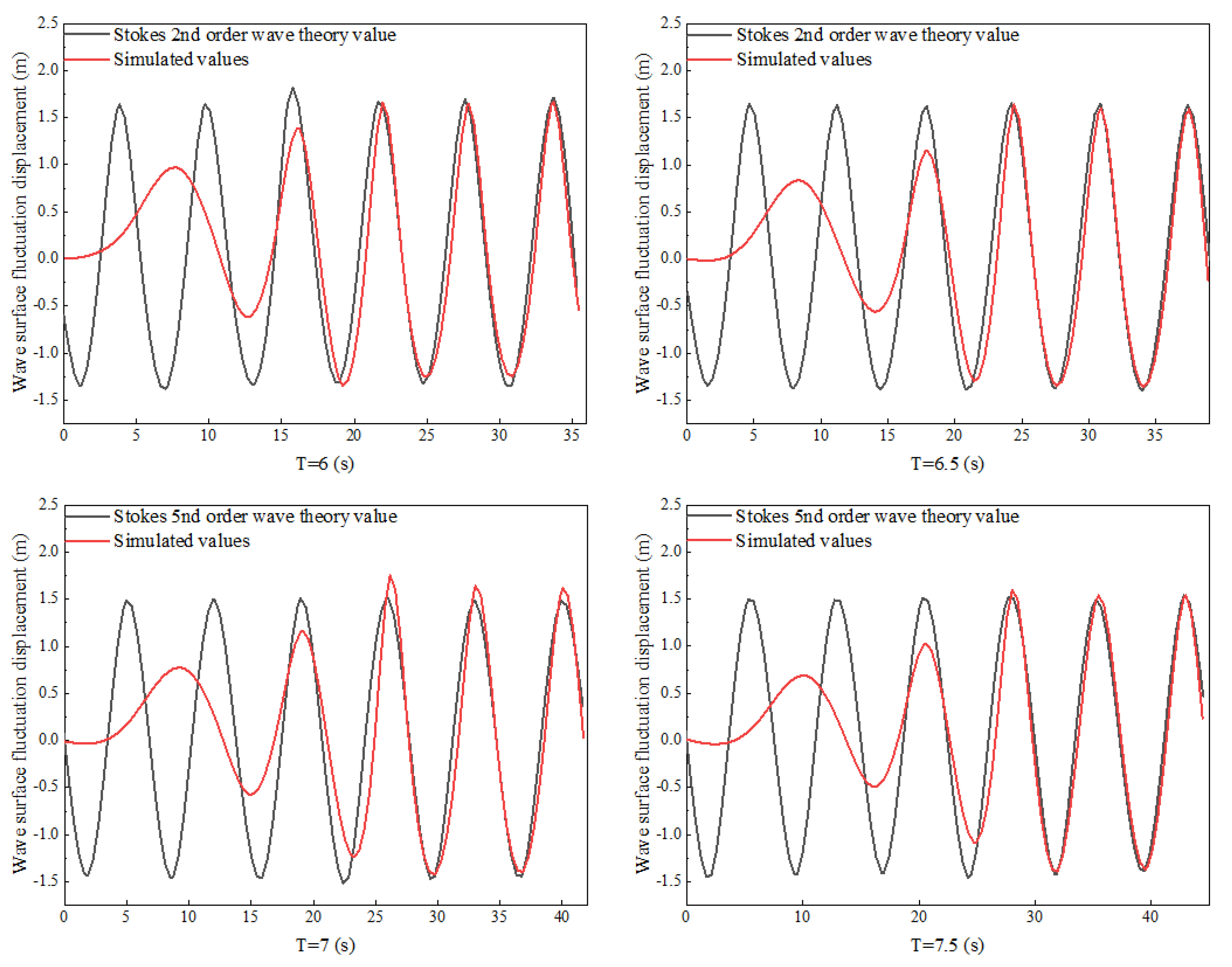
In the existing research on the joint action of seismic and wave energies on deep-water bridges, wave parameters are generally selected for specific sea areas. The wave heights taken in the previous section (at a water depth of 20 m and a wave height of 5 m) are already extreme sea conditions and extreme wave conditions, and most of the wave parameters selected in the existing studies are concentrated around 3 m [21]. Therefore, in the following discussion on the impacts of different wave periods on the pier, the wave height is taken as 3.0 m, the water depth is taken as 20 m and the wave periods are 6.0, 6.5, 7.0, 7.5, 8.0, 8.5 and 9.0 s.

The values of d and H corresponding to the waves at different periods are calculated, and Stokes’s second-order and fifth-order waves are determined in the range of applicability of wave theory to describe the 3D numerical waves to be simulated. The wave parameters at each period are shown in

Table 1. Parameters relating to wave flow with different wave periods.

Periodicity (m)	Pogo (s)	Water Depth (m)	Theory	Wavelength (m)	Frequency (rad/s)	Wave Number
6	3	20	Stokes2	55.1	1.043	0.115
6.5	3	20	Stokes2	63.4	0.964	0.097
7	3	20	Stokes5	72.5	0.897	0.084
7.5	3	20	Stokes5	81.2	0.834	0.085
8	3	20	Stokes5	89.7	0.781	0.071
8.5	3	20	Stokes5	97.8	0.735	0.064
9	3	20	Stokes5	106.5	0.691	0.591

.

For the 3D numerical wave tank, the length is taken as six wavelengths (6 L), and the width is taken as 15 m. The corresponding boundary conditions are set for the six boundaries of the numerical tank model, and the bottom and side boundaries are adopted as solid-wall boundaries that can slide. The upper surface uses a free liquid surface boundary. The consistent flow boundary is used at the wave outlet (right boundary), and the horizontal velocity function of the wave plate performing simple harmonic motion is input at the wave inlet [22]. To avoid the effect of wave reflection on wave height, the calculation time is cut off before the wave reaches the right boundary and begins to reflect, i.e., at six wave periods. In the calculated 3D numerical flume, the wave surface fluctuation displacement time course is extracted for a point at a distance L from the incident boundary.

Based on the Stokes2-order wave theory and the Stokes5-order wave theory, the wavelengths of a Stokes2-order wave and a Stokes5-order wave and the theoretical front wave displacement at a double wavelength (L) are solved via Matlab 2016b programming. The theoretical wave displacement is compared with the above numerical and modular values to verify the simulation effect of the wave. The results of the comparison are shown in Figure 5. It can be seen from the comparison of the figures that when the wave fully develops and reaches stability, the simulated wave front wave displacement modulus is in good agreement with the theoretical value obtained for different wave periods, indicating that the three-dimensional numerical flume can simulate a more ideal wave.

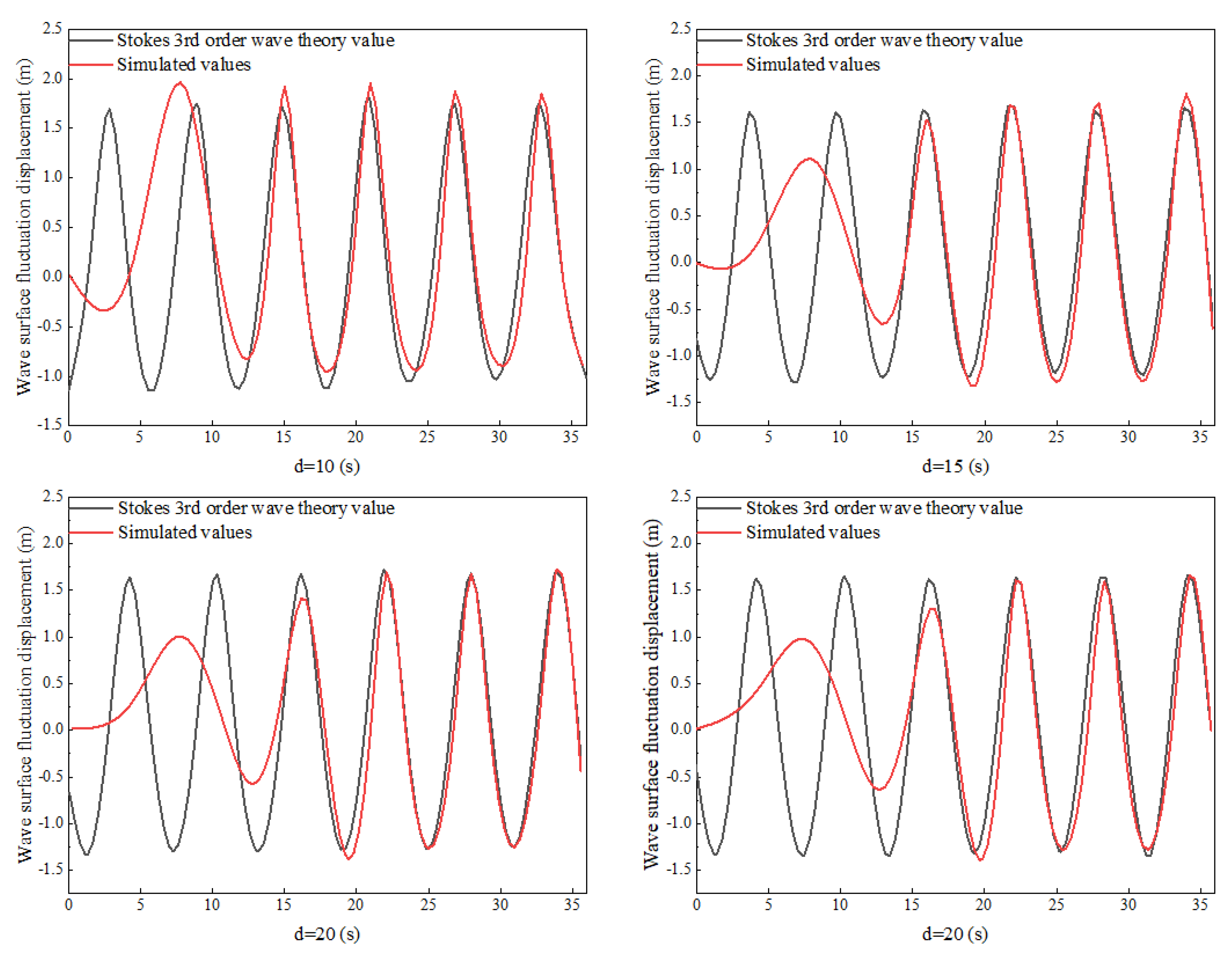
The wave parameters were selected as follows: a wave height of 3.0 m, a period of 16.0 s, and water depths of =10, 15, 20 and 25 m. The values of d and H corresponding to the waves at different water depths were calculated, and Stokes’s third-order waves were determined to describe the 3D numerical waves to be simulated in the applicable range of the wave theory [23].

Based on Stokes’s third-order wave theory, the wave surface fluctuation displacement times at the wavelength and doubled wavelength (L) of Stokes’s third-order wave are obtained via MATLAB programming, and the theoretical wave surface fluctuation displacement time is compared with the numerical mode value of the 3D wave simulated by the sink. The comparison results are shown in Figure 6. It can be observed from the comparison graph that when the waves are fully developed and stabilized, the simulated 3D numerical wave surface fluctuation displacement values are in good agreement with the theoretical values, especially at a water depth of 20 m.

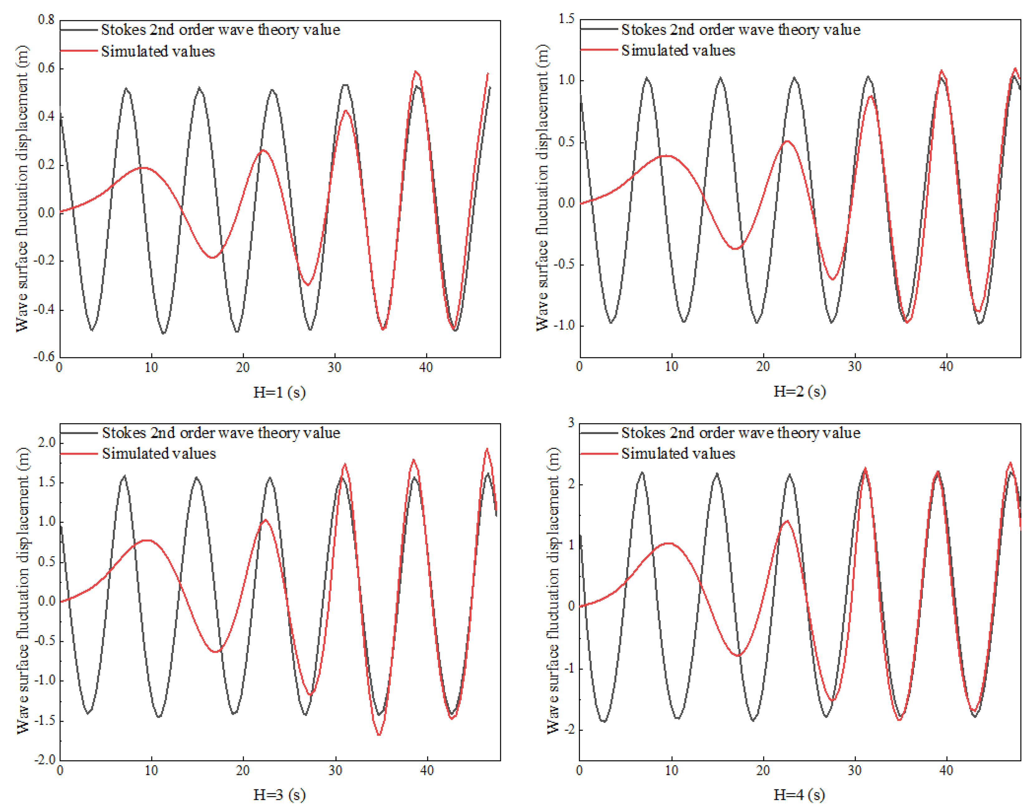
Limited by the insufficient water depth in the first two subsections, wave heights with a larger range of variation could not be simulated. Therefore, the wave parameters in this section are selected as follows: a period of 6.0 s, a water depth of 50 m, and wave heights of 1.0, 2.0, 3.0 and 4.0 m. The values of d and H corresponding to the waves at different wave heights are calculated, and Stokes’s second-order and third-order waves are determined in the applicable range of wave theory to describe the simulated 3D numerical waves. The relevant parameters for waves of different wave heights are shown in

Table 2. Parameters relating to wave flow with different wave heights.

Periodicity (m)	Pogo (s)	Water Depth (m)	Theory	Wavelength (m)	Frequency (rad/s)	Wave Number
1	8	50	Stokes2	99.5	0.786	0.062
2	8	50	Stokes2	99.4	0.786	0.061
3	8	50	Stokes3	100.3	0.786	0.062
4	8	50	Stokes3	101.4	0.786	0.062

.

Based on the wave concepts of Stokes’s second order and Stokes’s third order, the wavelengths of Stokes’s second-order and Stokes’s third-order waves and the wave floor displacement at the double wavelength (L) are obtained via MATLAB programming, and the theoretical values of the wave floor displacement are in contrast with the numerical mode values. The effects are provided in Figure 7. It can be seen that when the wave is absolutely developed and stabilized, the simulated 3D numerical wave floor displacements are in proper alignment with the theoretical values, mainly at the wave peak height of 3.0 m.

3.3. Bridge Foundation Grid Size

Using consistent settings for the wave parameters, boundary conditions, flume width and grid division, five different flume lengths (2 L, 3 L, 4 L, 5 L and 6 L) were selected for the model, and numerical calculations were extracted to compare the numerically simulated values of the wave surface fluctuation displacement time range at the distance L from the wave entrance with Stokes’s second-order wave theory values for different flume lengths. From the comparison, it is clear that the wave troughs do not fully develop when the flume length is 2 L and 3 L, and the waveform stabilizes when the flume length reaches 4 L in the direction of wave propagation [24]. Therefore, taking into account the model’s calculation efficiency and the simulated wave effect, the length of the water channel in the wave propagation direction is taken to be four times the wavelength (4 L).

In the numerical simulation of a wave–bridge pier for fluid–structure coupling, the pier cross-section size is small relative to the water length (4 L), and the waveform is not affected when the water length is taken to be 4 L. However, the pier’s cross-sectional size is not negligible with respect to the width of the water, and it will affect the wave crest line or trough line due to the blockage of the pier. For this reason, this section discusses the modeling details such as the width of the water column around the pier and the mesh size for the numerical simulation of a wave and bridge pier in fluid–structure coupling.

Figure 8 shows the distribution of the maximum value of the dynamic response of the pier column in different water width ranges. As can be seen from the figure, when the water on both sides of the pier column is 4 to 13 times the diameter of the pier column, the maximum value of the dynamic response of the pier column fluctuates greatly and cannot achieve a stable value. But when the width of the water on both sides of the pier column is greater than or equal to 14 times the diameter of the pier column (the data below the dashed line in the table), the dynamic response of the structure basically tends to stabilize the maximum values of the bending moment, force and displacement when the top action of the wave peak is 30.618 MN-m, 4.6833 MN and 3.490 cm or so up and down. The maximum values of the bending moment, shear force and displacement when acting at the bottom of the wave trough fluctuate up and down around 16.1140 MN-m, −2.7403 MN and −1.587 cm, respectively, and their fluctuation amplitudes are within the acceptable range [25]. As the excessive water body range will substantially increase the calculation time, taking into account the model’s calculation efficiency and accuracy factors, the width of the water body on both sides of the pier is taken to be 14 times its diameter in the subsequent coupled analysis of the pier and wave flow and solid coupling.

In an FSI numerical computation, the division of the computational domain’s model grid will have an impact on the computational accuracy, and the key to grid division is to ensure the accuracy of the computational results while considering the high demand on the computer and reducing the pressure on the computer. Mesh gradient partitioning is an effective method that can reconcile computational accuracy and computational efficiency. Therefore, the following will focus on the premise of encrypting the grid in the 4D water range around the pier column and will compare and analyze the grid division outside the 4D water range.

(1)

Discussion of the transitional water range on both sides of the perpendicular to the direction of wave propagation (Y-direction) mesh delineation:

The transitional water area around the pier column is 4D (its X- and Y-direction grid division is 8, and the width of the water body on the transitional water side is 30 m as a premise. Discuss the (i.e., Y-directional) meshing on both sides of the transition waters, and compare the effect of using isometric asymptotic meshing (10 copies; ratio = 3) with the above-mentioned consistent meshing (30 copies) on the calculation results.

Extract the dynamic response times (pier top displacement, pier bottom bending moment and pier bottom shear) of the pier column under different meshing methods, respectively. From the comparison, it can be seen that the calculation results of the water bodies on both sides of the transitional water range in the Y-direction using isometric gradient meshing are consistent with the calculation results of consistent meshing. Therefore, the water bodies on both sides of the transitional water range using isometric gradient meshing can meet the computational accuracy requirements while also greatly reducing the number of meshes, thereby improving the computational efficiency.

(2)

Discussion of the transitional water range on both sides of the wave propagation direction (X-direction) grid division:

The transition water area around the pier column is 4D (its X- and Y-direction mesh division is 8), and the width of the water body on the side of the transition water is 30 m as a premise. At the same time, perpendicular to the wave propagation direction (Y-direction), using isometric gradient meshing, discuss the X-direction meshing on both sides of the transition waters, and compare and analyze the impacts of different meshing on the dynamic response of the pier column [26].

The maximum values of the dynamic response of the pier column (pier top displacement, pier bottom bending moment and pier bottom shear) are extracted under different grid divisions, respectively. From the comparison, it can be seen that when the number of grid divisions of the X-directional water body on both sides of the transitional water range is greater than 40, the maximum value of the dynamic response of the pier tends to be stable. Therefore, taking into account the model’s computational efficiency and accuracy, in the later analysis of the pier–column–wave flow–solid coupling solution [27], the X-directional mesh division of the water bodies on both sides of the transitional waters with a side length of 4D is taken to be 40.

3.4. Simulation Analysis Model

In this paper, the SSTK-ω float mannequin (Shear Stress Transport k-ω Model) is used. This mannequin is an increased mannequin based totally on the k-ω model, and the k-ω mannequin and the Wilcox k-ω mannequin are mixed into one mannequin by introducing hybrid functions [28]. The expressions of turbulent kinetic power and dissipation charge transport equations in the SSTK-ω mannequin are proven in Equation (47).

$$\left\{\begin{array}{c}\frac{\partial (\rho k)}{\partial t}+u_i\frac{\partial (\rho k)}{\partial x_i}={\tau }_{ij}\frac{\partial u_i}{\partial x_j}-{\beta }^{*}\rho \omega k+\\ \frac{\partial }{\partial x_j}\left[\left(\mu +{\sigma }_k{\mu }_t\right)\frac{\partial k}{\partial x_j}\right]\\ \frac{\partial (\rho \omega )}{\partial t}+u_i\frac{\partial (\rho \omega )}{\partial x_i}=\frac{\gamma }{v_{\mathrm{T}}}{\tau }_{ij}\frac{\partial u_i}{\partial x_j}-\beta \rho {\omega }^2+\\ \frac{\partial }{\partial x_j}\left[\left(\mu +{\sigma }_{\omega }{\mu }_t\right)\frac{\partial \omega }{\partial x_j}\right]+\\ 2\rho \left(1-F_1\right){\sigma }_{\omega 2}\frac{1}{\omega }\frac{\partial k}{\partial x_j}\frac{\partial \omega }{\partial x_j}\end{array}\right.,$$

(47)

Since the double-cylindrical piers of this bridge are connected by crossbeams and cover beams, only the vibration in the cross-flow direction of the double-cylindrical piers as a whole is considered; the piers can then be simplified as a mass-damped spring system with the dynamic equations shown in Equation (48):

$$\ddot{y}+2\zeta {\omega }_0\dot{y}+{\omega }_0^{2}y=P_{\mathrm{y}}(t)/m,$$

(48)

As we can see from the previous paper, the Fluent calculation is based on a two-dimensional simulation of the bridge pier section, and the cross-flow fluid force P_y(t) can be considered the lift force per unit length of the bridge pier. By expressing P_y(t) as the lift coefficient C_L, Equation (48) can be rewritten as Equation (49).

$$\ddot{y}+2\zeta {\omega }_0\dot{y}+{\omega }_0^{2}y=\frac{1}{2}\rho U^2{C}_{\mathrm{L}}D/m,$$

(49)

In fact, as the bridge pier is a three-dimensional structure, the displacement response calculated by Fluent cannot truly reflect the displacement of the top of the pier. The influence of the pier’s own vibration pattern and the change in the water flow along the length of the pier should also be considered, so the displacement response obtained from the simulation analysis must be corrected. Cross-flow vibration stiffness is mainly provided by the pier, and compared to the main beam, the mass of the pier is negligible; then, the actual pier can be simplified to the top of the cantilever beam with a mass block. The length of the pier L = 15.5 m, and the depth of water entry L₁ = 6.5 m. Assuming that the incoming flow velocity is distributed in an inverted triangle along the length of the pier, the modified dynamic equation is

$$\ddot{y}+2\zeta {\omega }_0\dot{y}+{\omega }_0^{2}y=\overline{P}/m,$$

(50)

Equation (51) is the dynamic equation of the actual bridge pier. Then, Equation (50) can be rewritten as Equation (51).

$$\begin{array}{l}\ddot{y}+2\zeta {\omega }_0\dot{y}+{\omega }_0^{2}y=\hfill \\ {\displaystyle \underset{0}{\overset{L_1}{{\displaystyle \int }}}}\left(1-\cos \frac{\pi x}{2L}\right)\cdot {\left(\frac{x}{L_1}\right)}^2\mathrm{d}x\cdot \frac{1}{2}\rho U^2{C}_{\mathrm{L}}D/m\hfill \end{array},$$

(51)

Combined with Equations (49) and (51), the relationship between the displacement response of the top of the pier and the displacement response calculated by Fluent is shown in Equation (52).

$$\frac{y_{\mathrm{c}}(t)}{y_{\mathrm{f}}(t)}={\displaystyle \underset{0}{\overset{L_1}{{\displaystyle \int }}}}\left(1-\cos \frac{\pi x}{2L}\right)\cdot {\left(\frac{x}{L_1}\right)}^2\mathrm{d}x=0.27,$$

(52)

4. Dynamic Response of a Bridge Foundation under Wave–Current Coupling

Considering the calculation accuracy and efficiency, the grid discretization used in this paper is that the X-direction grid division of the water body on both sides of the transition water body with a side length of 4D is taken to be 40, as shown in Figure 9. The specific parameters of the bridge model and flow field used are shown in

Table 3. Bridge pier and flow field parameters.

Pier height	30
Radius	3
Materials	C40
Modulus of elasticity	3.25 × 1010
Poisson’s ratio	0.2
Density	2500
Quality	1,200,000
Water depth	5, 10, 15, 20
Horizontal flow rate	1, 2, 3, 4, 5, 6
Water Density	1025
Bulk modulus	1 × 1020
Dynamic viscosity coefficient	1.05 × 10−3

. The three-dimensional flow field area is a 200 m × 80 m × dm cuboid, the flow field is divided into non-uniform grids and the grid is encrypted near the pier column. Solid-wall boundaries are selected for the bottom and front interfaces of the flow field, and the left and right sides of the flow field are the water inlet and outlet, respectively. The interface between the pier and the fluid is a fluid–structure interface. The duration of the analysis was 45 s, the step size was 0.05, the speed increased linearly between 0 and 0.5 s and the required speed remained unchanged after 0.5 s.

The full bridge dynamic response calculation conditions are divided into six groups to study the effects of JCSS load combinations, and the conditions 1(4), 2(5) and 3(6) are JCSS load combinations taking the wind, wave and current as the main loads, respectively. The design base period of the cross-sea bridge is generally 100 a in order to consider the influences of the participating load periods. The participating load recurrence periods are taken to be 10 a and 5 a, respectively, i.e., Cases 1, 2 and 3 divide the design base period of 100 a into 10 segments for combination, while Cases 4, 5 and 6 divide the design base period of 100 a into 20 segments for combination. The detailed design parameters of the wind and wave elements are shown in

Table 4. Extreme wind wave flow design parameters.

Work Conditions	V10 (m/s)	Vb (m/s)	Hs (m)	vu (m/s)	vt (m/s)	v (m/s)
1	42.91	53.61	7.84	0.76	1.16	1.84
2	30.14	37.14	11.63	0.76	1.16	1.84
3	30.14	37.14	7.84	1.13	1.16	2.34
4	42.91	53.61	6.59	0.64	1.16	1.76
5	25.69	33.69	11.63	0.64	1.16	1.76
6	25.69	33.69	6.59	1.13	1.16	2.34

.

$$V_{\mathrm{b}}=V_{10}{\left(\frac{64.2}{10}\right)}^{\alpha },$$

(53)

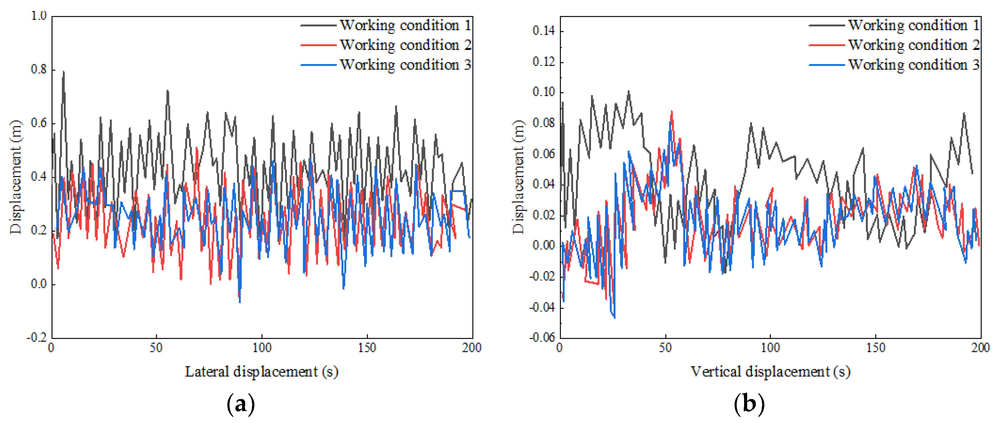
According to the JCSS combination rule, the wind, wave and current load combinations on the bridge were determined, and the dynamic response of the entire bridge to three combinations (conditions 1, 2 and 3) was calculated. In order to compare the effects of the three combinations on the bridge structure, the displacement response at the mid-span position of the main span, which is representative, was selected for analysis. The calculated results are shown in Figure 10.

From Figure 10a, it can be seen that the displacement response to the three operating conditions varies randomly with the time of the wind, wave and flow loads. The displacement amplitude is relatively larger in Case 1 with the wind as the main load, followed by Case 2 with a wave as the main load, and the amplitude is relatively small in Case 3, which took water as the main load. This is due to the fact that the wind load acts directly on the main girders, and according to the characteristics of the bridge, a wind speed point is placed every 6 m, and there are 198 wind speed points on the whole bridge; therefore, the wind load has a more obvious effect on the mid-span transverse displacement. In a 200 s load duration, the maximum values of the transverse displacement in the span are 0.84, 0.63 and 0.62 for cases 1, 2 and 3, respectively. However, there are still large transverse displacements, indicating that the influences of the waves and water flow on the transverse displacement in the main span cannot be ignored. It is also worth noting that the transverse displacement is basically positive; this is because the water current load is loaded in the same direction as the wave load.

From Figure 10b, it can be seen that the displacement responses in Case 2 and Case 3 basically overlap, while the displacement response in Case 1 is obviously large, and its vertical displacement maximum value is 22.2% and 22.4% higher than those of Case 2 and Case 3, respectively. This is because the wave flow load is the cross-bridge directional action, and the vertical displacement is mainly caused by the lifting force in the wind load. The average wind speed in Case 1 is the largest, while the average wind speeds in Case 2 and Case 3 are the same.

Figure 11 shows the time course of the transverse displacement of the main beam at the tower–beam union. The maximum values of transverse displacement in cases 1, 2 and 3 are 13.7%, 7.4% and 39.4% higher than those in cases 4, 5 and 6, respectively. Meanwhile, when the wave is the main load, the displacement response time histories of Case 2 and Case 5 are basically the same. This indicates that the wave has an obvious effect on the transverse displacement of the main beam at this location. In summary, it can be seen that the transverse displacement of the main beam is significantly reduced at the participating load return period of 5 when compared with 10 a. The environmental elements have different degrees of influence on the displacement response of the main beam at different locations, and when a load with significant influence on the response of the main beam is used as the main load (e.g., the wind load is used as the main load in the mid-span transverse displacement analysis), the influence of the participating load periods is relatively limited.

The wave movement traits change due to the presence of the current, which influences the wave pressure on the monopile. When the wave course is regular with a uniform water flow, the wave peak decreases and the wave steepness decreases, thus decreasing the wave pressure on the monopile. In addition, the mixed impact of a uniform water float pace and wave water first-class factor pace additionally impacts the drag pressure acting on the monopile, accordingly affecting the wave pressure on the monopile. The energy responses of the blended motion of the wave and uniform drift at distinctive waft velocities and the energy responses of the blended motion of wave and non-uniform float at specific go-with-the-flow velocities are analyzed, and their electricity responses at a one-of-a-kind float velocity are demonstrated in

Table 5. Dynamic responses of the monopile under the influence of waves and non-uniform flows with different flow velocities.

Flow Rate		Displacement (mm)		Shear Force (MN)		Bending Moment (MN·m)
		Waves, Uniform Flow	Waves, Non-Uniform Flow	Waves, Uniform Flow	Waves, Non-Uniform Flow	Waves, Uniform Flow	Waves, Non-Uniform Flow
Wave crest	1	0.28	0.27	0.49	0.11	2.84	2.91
	2	0.31	0.32	0.54	0.32	3.17	3.01
	3	0.38	0.33	0.64	0.74	3.71	3.11
	4	0.52	0.38	0.87	1.13	4.93	3.51
Wave Valley	1	−0.25	−0.24	−0.39	−0.43	−2.37	−2.34
	2	−0.22	−0.28	−0.34	−0.41	−2.16	−2.51
	3	−0.15	−0.27	−0.22	−0.37	−1.36	−2.36
	4	−0.08	−0.23	−0.06	−0.35	−0.58	−1.96

below.

As can be seen from Table 5 above, the maximum dynamic responses of the combined action of a wave and uniform flow and the combined action of a wave and non-uniform flow gradually increase with the increase in the flow velocity. Under the same flow velocity, the combined action of a wave and a uniform flow under a wave crest is greater than or equal to the combined action of a wave and a non-uniform flow, and the relationship between the two is opposite under a wave trough. Under the combined action of the two, the maximum dynamic response value of a single pile under the action of a wave crest is greater than the absolute value of the maximum response value under the action of a wave trough, which indicates that the non-uniform flow and the combined action of a uniform flow and a wave have strong nonlinearity.

5. Conclusions

In this paper, based on wave–flow coupling and Stokes’s wave theory, the dynamic responses of bridge foundations under deep-water conditions are analyzed. The SSTK-ω turbulence model is used to set up six working conditions and simulate various wave–flow coupling situations, different flow velocity waves and non-uniform flow effects, and the results of the dynamic response of the bridge foundation under different conditions are obtained. The specific conclusions are as follows:

• When the length of the water in the direction of wave propagation reaches four times the wavelength (4 L), the width of the water body on both sides of the pier is taken as more than 14 times its diameter, and the dynamic response of the pier column fluctuates less in the highest value and basically tends to be stable. Considering calculation accuracy and efficiency and the numerical analysis of the pier–wave coupling, the wave propagation direction of the water length is taken to be four times the wavelength (4 L), and the width of the water on both sides of the pier column is taken to be 14 times its diameter.
• The displacement responses in Case 2 and Case 3 basically overlap, while the displacement response in Case 1 is significantly larger, and its vertical displacement maximum value is 22.2% and 22.4% larger than the values for Case 2 and Case 3, respectively. The maximum values of the transverse displacement in Cases 1, 2 and 3 are 13.7%, 7.4% and 39.4% higher than those in cases 4, 5 and 6, respectively, while the displacement responses of Cases 2 and 5 are basically the same when the wave is the main load, which indicates that the wave has an obvious influence on the transverse displacement of the main beam at this location.
• In the combined action of a uniform flow and waves with different flow velocities, the maximum dynamic response value of a single pile increases with the increase in the uniform flow velocity, and the maximum dynamic response value of single pile is obtained at the peak and trough of the wave, indicating that the wave load plays a major role in the combined action. In the combined action of a non-uniform flow and waves with different flow velocities, the maximum dynamic response of a single pile gradually increases with an increase in the non-uniform flow velocity, and the maximum dynamic response of a single pile is also obtained at the positions of the wave’s crest and trough. Therefore, wave load plays a major role in the combined action.

In this paper, only the wave–current coupling is considered. In fact, there may be a variety of load coupling effects, such as wind, wave and current, on the bridge. Future research can begin with the dynamic responses of bridges to multiple-load coupling.

References

- Liu, C.; Wang, Y.; Hu, X.; Han, Y.; Zhang, X.; Du, L. Application of GA-BP neural network optimized by Grey Verhulst model around settlement prediction of foundation pit. Geofluids 2021, 2021, 5595277. [Google Scholar]
- Del Giudice, E.; Vitiello, G. Influence of gravity on the collective molecular dynamics of liquid water: The case of the floating water bridge. arXiv 2010, arXiv:1009.6014. [Google Scholar]
- Fuchs, E.C.; Agostinho, L.L.F.; Eisenhut, M.; Woisetschläger, J. Mass and charge transfer within a floating water bridge. Laser Appl. Life Sci. SPIE 2010, 7376, 393–407. [Google Scholar]
- Lieberherr, E.; Ingold, K. Actors in water governance: Barriers and bridges for coordination. Water 2019, 11, 326. [Google Scholar]
- Wu, A.J.; Yang, W.L.; Zhao, L. Analysis of dynamic response of deep-water bridge piers under the joint action of wave flow and earthquake. J. Southwest Jiaotong Univ. 2018, 53, 79–87. [Google Scholar]
- Mondal, M.S. Local Scour at Complex Bridge Piers in Bangladesh Rivers: Reflections from a Large Study. Water 2022, 14, 2405. [Google Scholar]
- Tan, Z.; Gou, H.; Pan, K.; Wang, J. Research on dynamic response of deepwater high-rise-pier continuous rigid-frame bridge during construction based on fluid-solid coupling. Bridge Constr. 2022, 52, 82–88. [Google Scholar]
- Abdelhaleem, F.S.; Mohamed, I.M.; Shaaban, I.G.; Ardakanian, A.; Fahmy, W.; Ibrahim, A. Pressure-flow scour under a bridge deck in clear water conditions. Water 2023, 15, 404. [Google Scholar]
- Fuchs, E.C.; Sammer, M.; Wexler, A.D.; Kuntke, P.; Woisetschläger, J. A floating water bridge produces water with excess charge. J. Phys. D Appl. Phys. 2016, 49, 125502. [Google Scholar] [CrossRef] [Green Version]
- Gogus, M.; Daskin, S.; Gokmener, S. Effects of collars on local scour around semi-circular end bridge abutments. In Proceedings of the Institution of Civil Engineers-Water Management; Thomas Telford Ltd.: London, UK, 2023; pp. 1–11. [Google Scholar]
- Cederwall, K.; Shady, A.; Björklund, G. Workshop 4 (synthesis): Bridge building between water and energy. Water Sci. Technol. 2002, 45, 149–150. [Google Scholar]
- Hua, X.G.; Deng, W.P.; Chen, Z.Q.; Tang, Y. Dynamic response of a concrete girder bridge with double cylindrical piers under the action of water flow. Eng. Mech. 2021, 38, 40–51. [Google Scholar]
- Perrier, E.; Kot, M.; Castleden, H.; Gagnon, G.A. Drinking water safety plans: Barriers and bridges for small systems in Alberta, Canada. Water Policy 2014, 16, 1140–1154. [Google Scholar]
- Nguyen, L.D.; Dang, P.D.N.; Nguyen, L.K. Estimating surface water and vadose water resources for an ungauged inland catchment in Vietnam. J. Water Clim. Change 2021, 12, 2716–2733. [Google Scholar]
- Al-Omaria, A.; Al-Hourib, Z. Impact of greywater reuse on black water quality. Desalination Water Treat. 2021, 218, 240–251. [Google Scholar]
- Rijsberman, F.; Mohammed, A. Water, food and environment: Conflict or dialogue? Water Sci. Technol. 2003, 47, 53–62. [Google Scholar]
- Fang, C.; Li, Y.; Xiang, X.; Zhang, J. Effects of wind, wave, and current load combinations on the dynamic response of cross-sea bridges. J. Southwest Jiaotong Univ. 2019, 54, 908–914. [Google Scholar]
- Li, R.; Chen, Z.; Wu, K.; Xu, J. Shale gas transport in nanopores with mobile water films and water bridge. Pet. Sci. 2023, 20, 1068–1076. [Google Scholar]
- Alvarado, J.; Siqueiros-García, J.M.; Ramos-Fernández, G.; García-Meneses, P.M.; Mazari-Hiriart, M. Barriers and bridges on water management in rural Mexico: From water-quality monitoring to water management at the community level. Environ. Monit. Assess. 2022, 194, 912. [Google Scholar]
- Wang, X.; Dong, Z.; Wang, W.; Tan, Y.; Zhang, T.; Han, Y. Regional water allocation for coordinated development among the social, economic and environmental systems. J. Water Supply Res. Technol. Aqua 2021, 70, 550–569. [Google Scholar]
- Drioli, E.; Ali, A.; Lee, Y.M.; Al-Sharif, S.F.; Al-Beirutty, M.; Macedonio, F. Membrane operations for produced water treatment. Desalination Water Treat. 2016, 57, 14317–14335. [Google Scholar]
- Liu, Z.; Wang, X.; Song, J.; Roy, T.; Li, S.; Liu, J.; Huang, L.; Liu, X.; Jin, Z.; Zhao, D. Pouring-type gravity-driven oil–water separation without water bridge. Micro Nano Lett. 2017, 12, 744–748. [Google Scholar] [CrossRef]
- Wang, C.; Xing, Y.; Lei, Y.; Xia, Y.; Zhang, C.; Zhang, R.; Wang, S.; Chen, P.; Zhu, S.; Li, J.; et al. Adsorption of water on carbon materials: The formation of “water bridge” and its effect on water adsorption. Colloids Surf. A Physicochem. Eng. Asp. 2021, 631, 127719. [Google Scholar]
- Bakr, A.R.; Fu, G.Y.; Hedeen, D. Water quality impacts of bridge stormwater runoff from scupper drains on receiving waters: A review. Sci. Total Environ. 2020, 726, 138068. [Google Scholar] [PubMed]
- Timmerman, J.G.; Beinat, E.; Termeer, C.J.A.M.; Cofino, W.P. A methodology to bridge the water information gap. Water Sci. Technol. 2010, 62, 2419–2426. [Google Scholar] [CrossRef]
- Gao, Y.; Liu, Z.; Ge, H.; Sun, J.; Yin, R. Dynamic Response Analysis of Pier under Combined Action of Wave and Current. CICTP 2020 2020, 2020, 1316–1327. [Google Scholar]
- Wang, C.N.; Yang, F.C.; Nguyen, V.T.T.; Vo, N.T.M. CFD analysis and optimum design for a centrifugal pump using an effectively artificial intelligent algorithm. Micromachines 2022, 13, 1208. [Google Scholar]
- VOTMN. Centrifugal pump design: An optimization. Eurasia Proc. Sci. Technol. Eng. Math. 2022, 17, 136–151. [Google Scholar] [CrossRef]
Figure 1.
Bridge plan layout.
Figure 2.
First- and second-order volume wavefront elevation.
Figure 3.
River cross-section.
Figure 4.
Time course curve of fluctuation displacement at each point.
Figure 5.
Comparison of wave theory and simulated values for different periods.
Figure 6.
Comparison of theoretical and simulated values of waves at different water depths.
Figure 7.
Comparison of theoretical and simulated values of wave flow with different wave heights.
Figure 8.
Distribution of the maximum value of the dynamic response of the bridge foundation for different water width ranges.
Figure 9.
Mesh discretization on both sides of the piers.
Figure 10.
Different combinations of mid-span displacements.
Figure 11.
Comparison of lateral displacement at the bridge joint.