
ICA-LightGBM Algorithm for Predicting Compressive Strength of Geo-Polymer Concrete


1
School of Mines, China University of Mining and Technology, Xuzhou 221008, China
2
Shandong Energy Group Luxi Mining Co., Ltd., Heze 250101, China
3
Faculty of the Engineering, Tarbiat Modares University, Jalal AleAhmad, Nasr, Tehran 14115-175, Iran
4
School of Civil and Environmental Engineering, University of Technology Sydney, Sydney, NSW 2007, Australia
5
School of Civil Engineering, Guangzhou University, Guangzhou 511370, China
*
Authors to whom correspondence should be addressed.
Buildings 2023, 13(9), 2278; https://0-doi-org.brum.beds.ac.uk/10.3390/buildings13092278
Submission received: 14 August 2023
/
Revised: 31 August 2023
/
Accepted: 5 September 2023
/
Published: 7 September 2023
(This article belongs to the Special Issue Cement and Concrete Research)
Abstract
:The main goal of the present study is to investigate the capability of hybridizing the imperialist competitive algorithm (ICA) with an intelligent, robust, and data-driven technique named the light gradient boosting machine (LightGBM) to estimate the compressive strength of geo-polymer concrete (CSGCo). The hyper-parameters of the LightGBM algorithm have been optimized based on ICA and its accuracy improved. The obtained results from the proposed hybrid ICA-LightGBM are compared with the traditional LightGBM model as well as four different topologies of artificial neural networks (ANN) comprising a multi-layer perceptron neural network (MLP), radial basis function (RBF), generalized feed-forward neural network (GFFNN), and Bayesian regularized neural network (BRNN). The results of these models were compared based on three evaluation indices of R2, RMSE, and VAF for providing an objective evaluation of the performance and capability of the predictive models. Concerning the outcomes, the ICA-LightGBM with the R2 of (0.9871 and 0.9805), RMSE of (0.4703 and 1.3137), and VAF of (98.5773 and 98.0397) for training and testing phases, respectively, was a superior predictor to estimate the CSGCo compared to the LightGBM with the R2 of (0.9488 and 0.9478), RMSE of (0.9532 and 2.1631), and VAF of (94.3613 and 94.5173); the MLP with the R2 of (0.9067 and 0.8959), RMSE of (1.3093 and 3.3648), and VAF of (88.9888 and 84.9125); the RBF with the R2 of (0.8694 and 0.8055), RMSE of (1.4703 and 5.0309), and VAF of (86.3122 and 66.1888); the BRNN with the R2 of (0.9212 and 0.9107), RMSE of (1.1510 and 2.6569), and VAF of (91.4168 and 90.5854); and the GFFNN with the R2 of (0.9144 and 0.8925), RMSE of (1.1525 and 2.9415), and VAF of (91.4092 and 88.9088). Hence, the proposed ICA-LightGBM algorithm can be efficiently used in anticipating the CSGCo.
1. Introduction
In the last decade, there has been significant progress made by mankind toward a range of vital goals related to its development. Building infrastructure can be able to lead to the establishment of a community [1,2,3]. According to Murthy and Rai [4], the buildings industry serves a crucial role in the evolution of civilization. Concrete is one of the vital building components that should be used whenever any sort of structure is being created. Compared to traditional concrete, which has been utilized extensively in residential construction over the last three decades, eco-friendly concretes are a kind of materials that totally replace cement with ground granulated blast furnace slag (GGBFS), fly ash, and alkaline solutions [5,6]. After water, concrete is the second most significant possible application on our planet. Furthermore, cement is the important binding component in the elements of conventional concrete, and the manufacturing of one ton of cement results in the discharge of about one ton of CO2 into the atmosphere. When making geo-polymer concrete, the cement can be substituted by GGBFS and fly ash. In concretes, the component with the higher emissions is cement. Hence, using geo-polymer concrete can decrease traditional concrete’s environmental impact by approximately eighty percent.
According to the Central Electricity Authority [7], emissions of CO2 are having a significant effect on the temperature of the earth. In conclusion, sustainable development is crucial for the future of buildings [8]. In terms of cost, a geo-polymer is more cost-effective compared to normal concrete. It leads to a cost decrement that is between thirty-five and forty percent lower than the original price. According to Verma and Dev [9], geo-polymer concrete outclasses common concretes in points of both its strength and its endurance. This makes it a potential replacement for traditional concrete. It is required to employ a solution with alkaline contents for activating the pozzolanic compound that is utilized in geo-polymer concrete so that it can be used to form bonds. The use of fly ash, slag, or metakaolin components in geo-polymer concretes allows for the total elimination of cement. As examples of alkaline materials, one may consider using sodium hydroxides or silicates. Interactions and relationships formed using geo-polymer concretes are unique in comparison to those that are produced using ordinary concrete. The term “geopolymer” was first used to describe the relationship that was formed as a result of these events. The effectiveness of geo-polymer concrete in experiments has been demonstrated to be more effective than that of traditional concretes, which suggests that it might be the best replacement for traditional concretes. It is achievable that this is the future of environmentally responsible construction and infrastructure [8].
A diverse variety of properties and variables may have an effect on the amount of strength possessed by geo-polymer concrete, involving both parameters related to concrete structure and external parameters. Temperature, length, various methods of curing, humidity, and air confinement all have vital roles in the external variables, whilst the characteristics of the components and the diverse composition are accounted for in the parameters related to concrete structure [10]. According to Borges et al. [11], the chemistry of the binders and the dimensions of their particulates are essential elements in both the beginning of the response and its development later on, when it becomes more pronounced; however, the proportions of these two parameters additionally have an essential role in the capability to manage the strength in line with the regulations. The slag percentage improvement in the formulation enhances the naturally cured geo-polymer concrete compressive strength [12,13,14,15]. Because of the higher surface area available, the smaller fragments of fly ash and slag respond quickly, which increases the initial strength of the concrete [16]. According to Verma and Dev [17], the ratio of liquid to binder additionally serves an essential role in the reaction and makes it difficult to determine the strength. The geo-polymer process necessitates the presence of water; however, this water will dissipate as the process hardens and is thus not necessary for the outcome of the process. Because of this, just a relatively small quantity of water is needed for the reaction with all of the elements of geo-polymer concrete. Strength in geo-polymer concrete is inversely proportional to the amount of liquid used in the mixture [18]. Given the superior suitability of Sulphonated-Naphthalene-Formaldehyde-based superplasticizers for bodies of geo-polymer concrete, choosing and employing superplasticizers in geo-polymer concrete serves an essential part in the formation of bonds [19]. When it involves establishing the geo-polymer process, the potency and concentration of the alkaline solution are of the utmost importance. Concrete’s performance and strength are strongly impacted by the response that occurs, which is closely corresponded to the molarity of sodium or potassium hydroxide [19]. Oven-cured materials are readily obtained stronger than atmospheric-cured samples, according to research by Chouksey et al. [20] and Verma [21]; hence, cured temperature and circumstances are also highly beneficial when it comes to achieving the desired design strength. In addition to this, geo-polymer concrete is exceptionally resistant to the damaging effects of harsh environments [18,22,23]. Therefore, geo-polymer concrete could involve a period of environmentally responsible growth in the building sector. The use of geo-polymer concrete may take various forms in a variety of contexts around the globe.
In order to determine the compressive strength of geo-polymer concrete, many attempts have been conducted in a laboratory (which is also called direct determination). However, sample preparation and test conducting is time consuming and costly [24,25,26,27] and because of that some researchers [28,29,30,31,32] tried to propose machine learning models to solve this problem. In addition, these techniques have been successfully used in the other applications of civil engineering [33,34,35,36,37,38,39,40,41]. Therefore, the authors decided to use a novel hybrid model of LightGBM mixed with the imperialist competitive algorithm (ICA) for prediction of the compressive strength of geo-polymer concrete. The following sections will discuss the background and details of this novel technique and its performance with details.
2. Materials and Methods
2.1. LightGBM
LightGBM is a decision tree structure that utilizes an original boosting system. Within the conventional GBDT, LightGBM integrates 2 novel strategies: gradient-based one-side sampling (GOSS) and exclusive feature bundling (EFB) [42]. Hence, it demonstrates a quicker training rate, greater precision, and better efficiency in comparison to the GBDT and extreme gradient boosting (XGBoost) [43]. In the context of the GOSS approach, it becomes feasible to eliminate a substantial portion of samples by utilizing modest gradients. This allows LightGBM to construct its models using the available data, calculating an information gain more efficiently. The GOSS approach can be more precise and successful than the conventional GBDT method whenever used for a small-scale dataset because a dataset with huge gradients is more significant for information acquisition. Concerning the EFB, it permits the bundling of features that are incompatible with one another in order to lower the total number of characteristics. Furthermore, the application of the pre-sorting technique is the stage of the classic GBDT technique that consumes an enormous amount of time. This approach begins by enumerating all of the potential features based on the ranking values of features and then proceeds to locate the best-dividing part, which requires a significant amount of time and computer memory [44]. LightGBM, on the other hand, employs the histogram algorithm and leaves growing techniques as an alternative to the conventional pre-sorting approach in order to lessen the amount of memory used and the amount of time spent on the process, hence accelerating computing. The Light-GBM algorithm’s framework is represented in Figure 1, which may be found here. The LightGBM technique yields algorithmic controlling and optimizing with the main hyper-parameters shown in Figure 2.
2.2. ICA
The first imperialist competitive algorithm (ICA) was created by Atashpaz-Gargari and Lucas [45], as a metaheuristic algorithm to address or handle different minimizing or maximizing problems. ICA operates in a manner similar to that of other metaheuristic algorithms; it takes into account the swarm of the world, or the number of countries, and treats each country as a potential answer. The construction of the method proceeds by selecting a random number of countries to use as beginning results. The members of the population in ICA are represented by different countries; from this group, the strongest nations, or those with the greatest amount of strength, are chosen to take on the role as imperialists. The other nations fulfill the function of imperialists’ swarms in this scenario. The countries in the ICA that have the lowest operating costs are the most powerful because they are able to acquire ownership or manage over the most swarms. As a rule, the ICA is composed of three basic mechanisms or operations, and they are assimilation, revolution, and competition. The assimilation mechanisms lead the swarms toward the goal of becoming imperialists in order for them to attain more authority and power, a higher cultural level, and an improved economic situation. If the swarms are successful in attaining a location that is superior to that of their imperialists during the first two operators, then they will be in a location to assume control of the empire. Last but not least, throughout the course of the rivalry, the imperialists will also have a good possibility of acquiring more colonies. Throughout the course of the competition, the empire that is the least powerful will eventually fall, while the empires that are the most powerful will be able to acquire ownership of further colonies, leading to a rise in their authority and strength. The process described above is continued until either the most powerful empire or no empire at all can successfully govern all nations (Figure 3). Under these circumstances, the remaining empires will succumb to their inherent weakness, which will result in their transformation into colonies.
3. Data Analysis
Fly ash, sodium silicate, sodium hydroxide, fine aggregates, coarse aggregates, superplasticizers, and water are the components that are used in the production of geo-polymer concretes. Prior to the manufacturing of concrete on an enormous scale, labs consistently conduct quality inspections to ensure that the raw ingredients are of an acceptable standard. Fly ash is almost always acquired from the chemical industry, whereas alkaline solutions and superplasticizers are usually sourced from the power plant that is geographically located closest to the facility. Both coarse and fine aggregates are sourced from resources that are readily accessible in the area. Water gets utilized in accordance with the requirements that are necessary in that region and are accessible. The production of the alkaline solutions occurs before 20–24 h of the mixture. Since combining in mixers consumes more than hand combining, geo-polymer concrete cannot be prepared as quickly as traditional concrete. M-sand has a wide range of potential applications in geo-polymer concretes. The adequate-graded pieces in it provide superior outcomes compared to regular sand because of this.
In order to determine what materials were present in the data cases, an X-ray fluorescence spectroscopy (XRF) analysis was performed on fly ash as well as additional pozzolanic components. Due to this, the proportions of alumina, silica, and sodium oxide in the mixture had to be determined. When obtaining chemicals from various companies, one would be given the amount of minerals or a minimum analysis of the chemical solutions. Laboratory testing was used to identify the size of the particles, bulk density, and other required characteristics. All of these trials had to be performed first before any more progress could be made with the mixed composition of the concretes.
In this study, 11 input parameters were used for predicting CSGCos, and the required database was gathered from research conducted by Verma [8]. The study being discussed right now is intended to identify a plan that helps engineers in improving various parts of geo-polymer concrete that are available for building operations. Parameters (both inputs and outputs) were given numerical values, and their descriptive statistics are shown in Table 1. In this study, a total of 61 laboratory tests were conducted in order to acquire the required data. The fly ash, rest period, curing temperature, curing period, NaOH/Na2SiO3, superplasticizer, extra water added, molarity, alkaline activator/binder ratio, coarse aggregate, and fine aggregate were considered as the input parameters that would be utilized in order to train the artificial intelligence models, whereas the CSGCo was imported into the models as the target of artificial intelligence modeling. The histogram chart of parameters is illustrated in Figure 4. This figure shows that the number of CSGCo in the range of 40–45 MPa is 22 cases. Furthermore, the heatmap correlation coefficient of parameters is displayed in Figure 4. Generally, the correlations between two parameters are determined with the Pearson correlation coefficient (r, r ∈ [−1, 1]). The Pearson correlation coefficient is specified applying the below equation [46]:
In which n, xm, and ym refer to the number of raw data samples, average value across all x data, and average value across all y data, respectively. If r is more than zero (r > 0), this means there is a positive linear correlation between the two parameters; the closer r is to one (r ≃ 1) represents a stronger positive linear correlation. On the other hand, if r is less than zero (r < 0), this signifies that there is a negative linear correlation between the two parameters; the closer r is to minus one (r ≃ −1) represents a stronger negative linear correlation [47].
Based on Figure 4, the coarse aggregate, curing temperature, and fly ash denote a positive linear correlation with the CSGCo, whereas the rest period, curing period, NaOH/Na2SiO3, superplasticizer, extra water added, molarity, alkaline activator/binder ratio, and fine aggregate demonstrate a negative linear correlation with CSGCo. Moreover, based on the absolute value of the Pearson correlation coefficient, it can be seen in Figure 5 that the curing period, superplasticizer, extra water added, and fine aggregate have a significant negative linear correlation and the coarse aggregate has a significant positive linear correlation with CSGCo, and the correlations of the rest inputs to CSGCo is weak to medium.
4. Pre-Analysis and Data Preparation
The following is the most important part of this paper: following the presentation of the basis of the gathered datasets and a summary investigation of the properties of the dataset, the compressive strength of geopolymer concrete data was divided into two main categories, the training set, which contains eighty percent of the whole concrete data (49 data samples), and the testing set, which contains twenty percent of the concrete data (12 data samples). After that, the LightGBM algorithm is fitted using the data from the training part. During this interim period, the ICA metaheuristic algorithm was used in order to determine the optimal values for the LightGBM model’s hyper-parameters. The RMSE is the objective function of ICA. This is the difference between the actual compressive strength of geopolymer concrete data on the training set and the obtained compressive strength of geopolymer concrete with the LightGBM technique utilizing the inputs of the training set. The following description provides an outline of the framework of the objective function.
In which Fr and are respectively measured and predict the compressive strength of geopolymer concrete. In this equation, . fit(trainingset), in which and show the hyper-parameters of learning_rate and colsample_bytree in the LightGBM algorithm and the LightGBM is fitted on the training data points.
In the last step of the process, the possible solutions of the ICA method are evaluated on the testing set using various statistical indices, which allows for the determination of the best hyper-parameters for the LightGBM system. In addition, the cosine amplitude approach is used to further elaborate the sensitivity analysis of the compressive strength of geopolymer concrete to the effective parameters. This analysis is based on the well-established LightGBM model, which has optimal values for its hyper-parameters.
5. Prediction Results
5.1. Hyper-Parameters’ Tuning
When learning soft computing techniques, one of the most essential duties is called hyper-parameter tuning. This reduces the likelihood of the algorithm being overfitted, improves its capacity to generalize, and reduces the model’s overall level of complexity. In the current research, the applied dataset was randomly classified into a training part including 80% of the geo-polymer concrete data and a test part including 20% of the geo-polymer concrete data in order to develop the LightGBM method. The correctness of the LightGBM model that was produced is evaluated with the help of the testing part, whereas the contribution of the training part is utilized to develop the algorithm in the first place. As was said before, in order to create the LightGBM method, two-tuple hyper-parameters, namely learning_rate and colsample_bytree, require their values to be adjusted. These values can be found in the model’s configuration file. Consequently, the ICA was used so that these two hyper-parameters could be optimized. The Ncountry, Ndecade, and Nimp values in the ICA were adjusted to 270, 350, and 25, respectively, and the number of iterations was set to 500. The ranges for the two hyper-parameters that define the bounds are (0.012, 0.55) and (0.15, 1.0), respectively, for learning_rate and colsample_bytree. Nevertheless, the generalization efficiency of the hybrid LightGBM system was evaluated using a ten-fold cross-validation approach, which was employed throughout the training phase of this study. ICA-LightGBM’s learning outcomes are illustrated in Figure 6, which can be seen here. It is clear that the ICA-LightGBM system did not begin to converge again before around 300 iterations were completed. In the end, the values acquired for the two hyper-parameters that were determined to be optimum are learning_rate = 0.32 and colsample_bytree = 0.97, respectively.
5.2. Evaluation of the Proposed Model
The most crucial thing to accomplish is to assess the capability of the developed models once the training of the model has been completed and the optimum hyper-parameters have been obtained. As a result, in order to evaluate the efficacy of the method, the coefficient of determination (R2), the root mean squared error (RMSE), and the variance accounted for (VAF) were used as assessment measures. When executing a regression employment, these three indices are usually employed as indicators for measuring the success of the artificial intelligence models, which can be derived using the following formulas [48,49,50,51]:
In this equation, Oi represents the actual values, Pi represents the projected values, is the average of the projected values, and n is the number of datasets. Notable is the fact that the values one, zero, and one hundred for R2, RMSE, and VAF, respectively, demonstrate a model with the highest efficiency and accuracy.
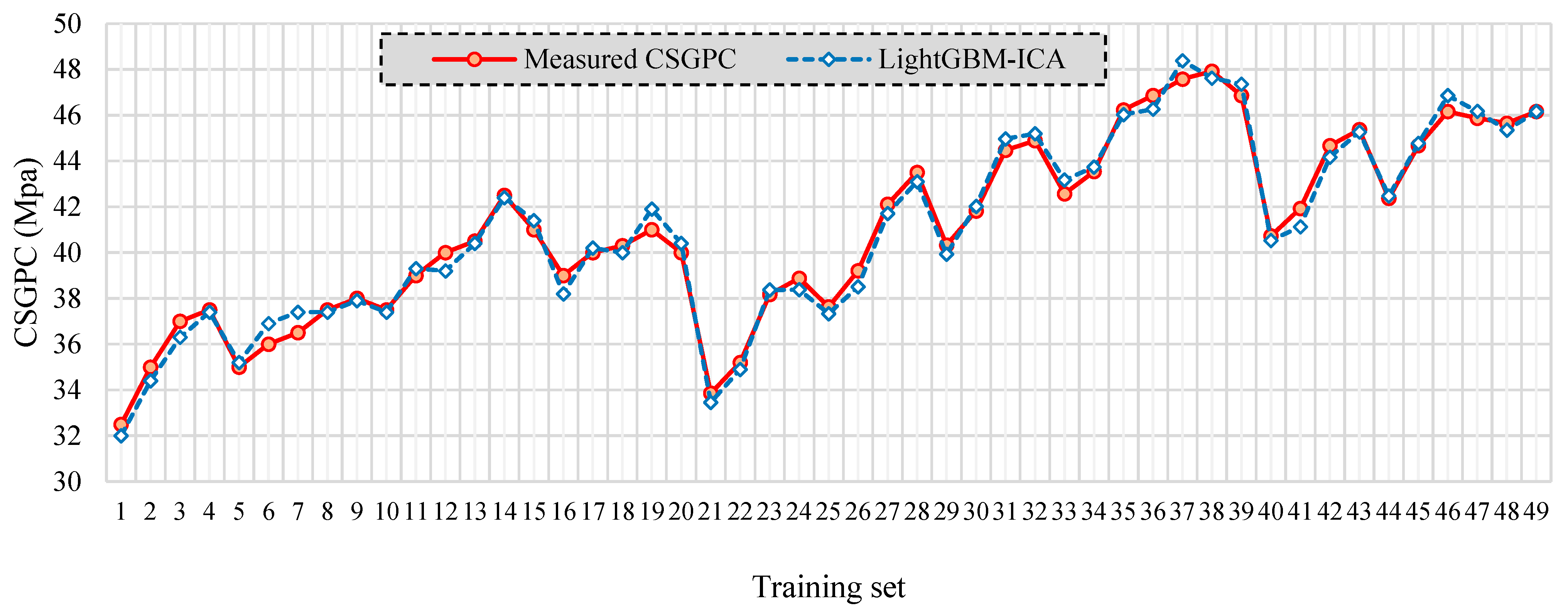
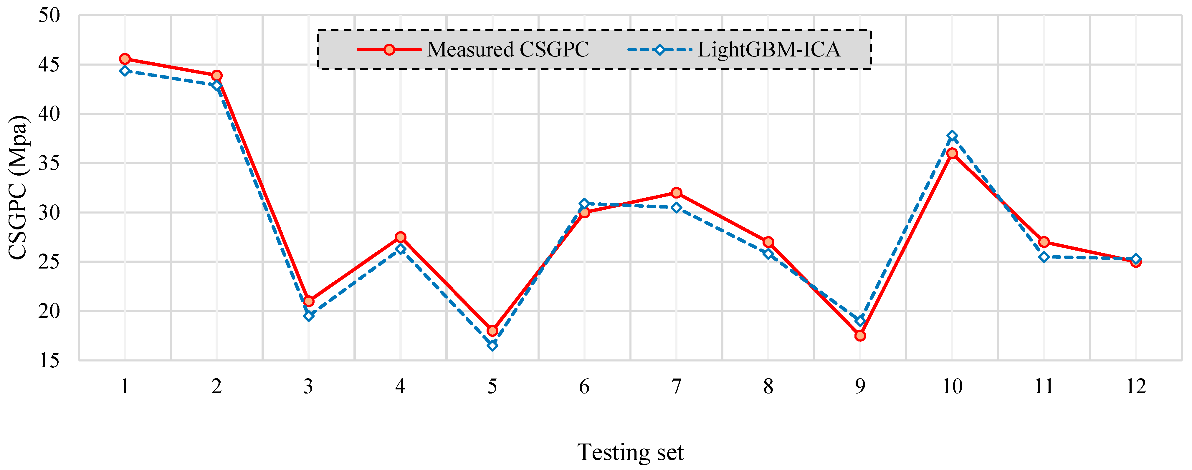
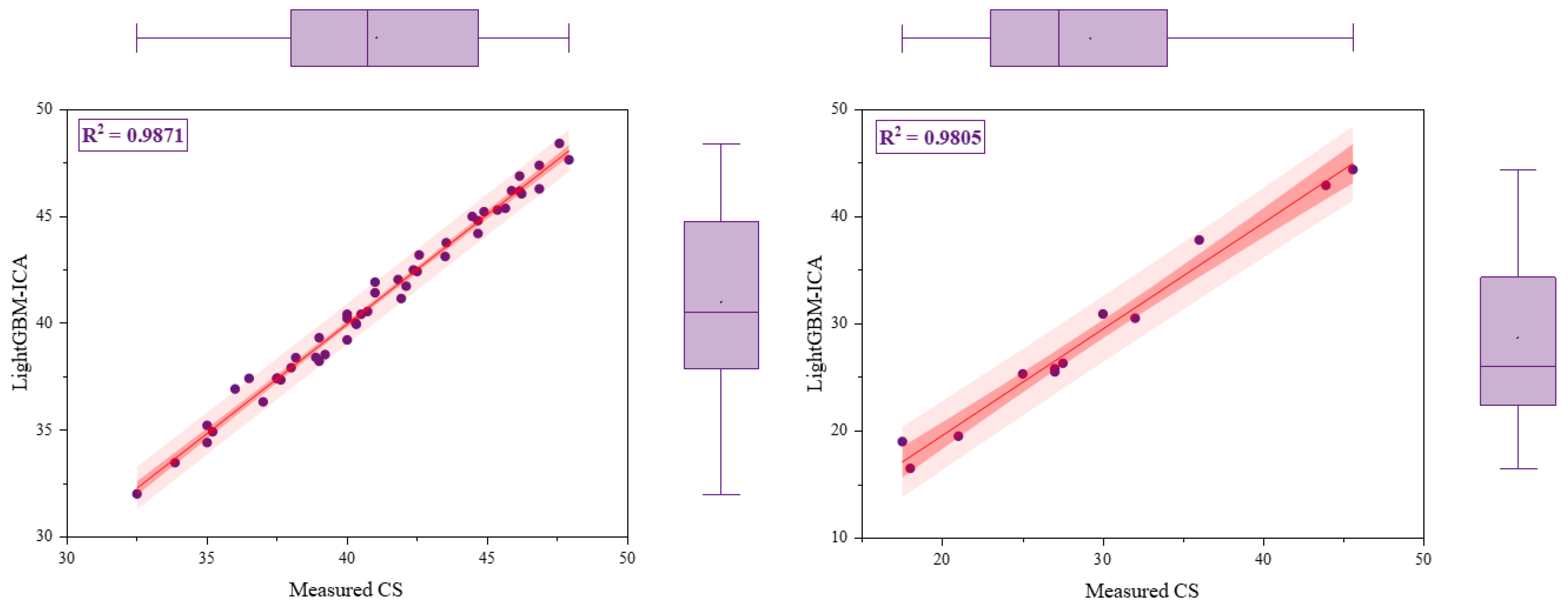
In light of this, the results of the calculations for the three evaluation indices of the ICA-LightGBM technique are as follows: on the training part, the R2 value is 0.9871, the RMSE value is 0.4703, and the VAF value is 98.5773; on the testing part, the R2 value is 0.9805, the RMSE value is 1.3137, and the VAF value is 98.0397. It is clear that the constructed ICA-LightGBM technique possesses outstanding precision and can accurately forecast the CSGCo. Furthermore, it was discovered that the model’s superiority on the testing part somewhat outperformed that on the training part. In Figure 7, you can see a comparison between the CSGCo that was anticipated using the ICA-LightGBM model and the CSGCo that was really measured. From a logical point of view, most of the projected CSGCo values are quite close to the actual CSGCo values.
6. Results and Discussion
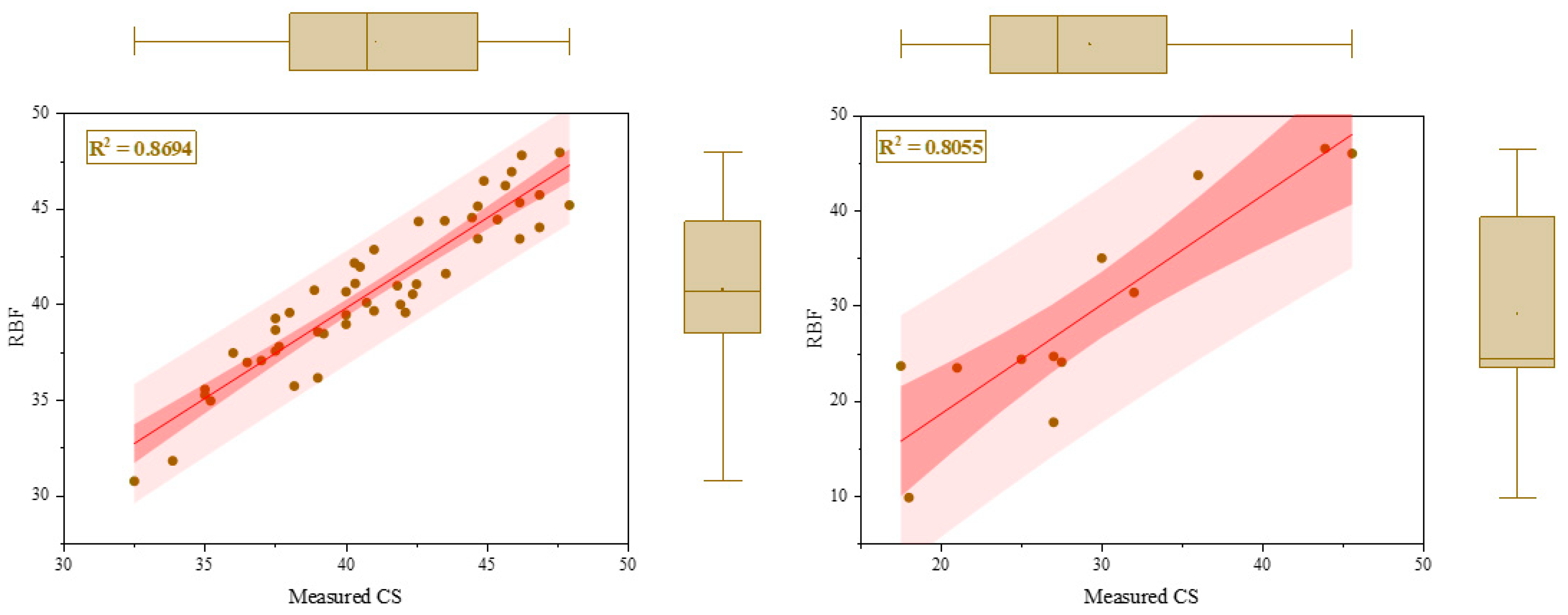
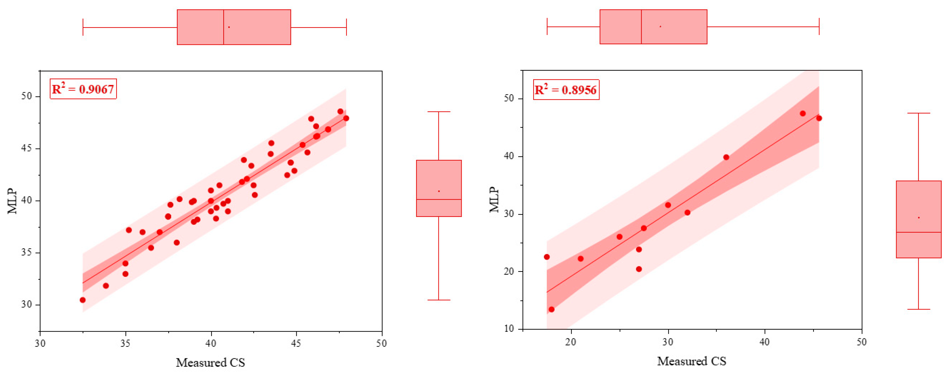
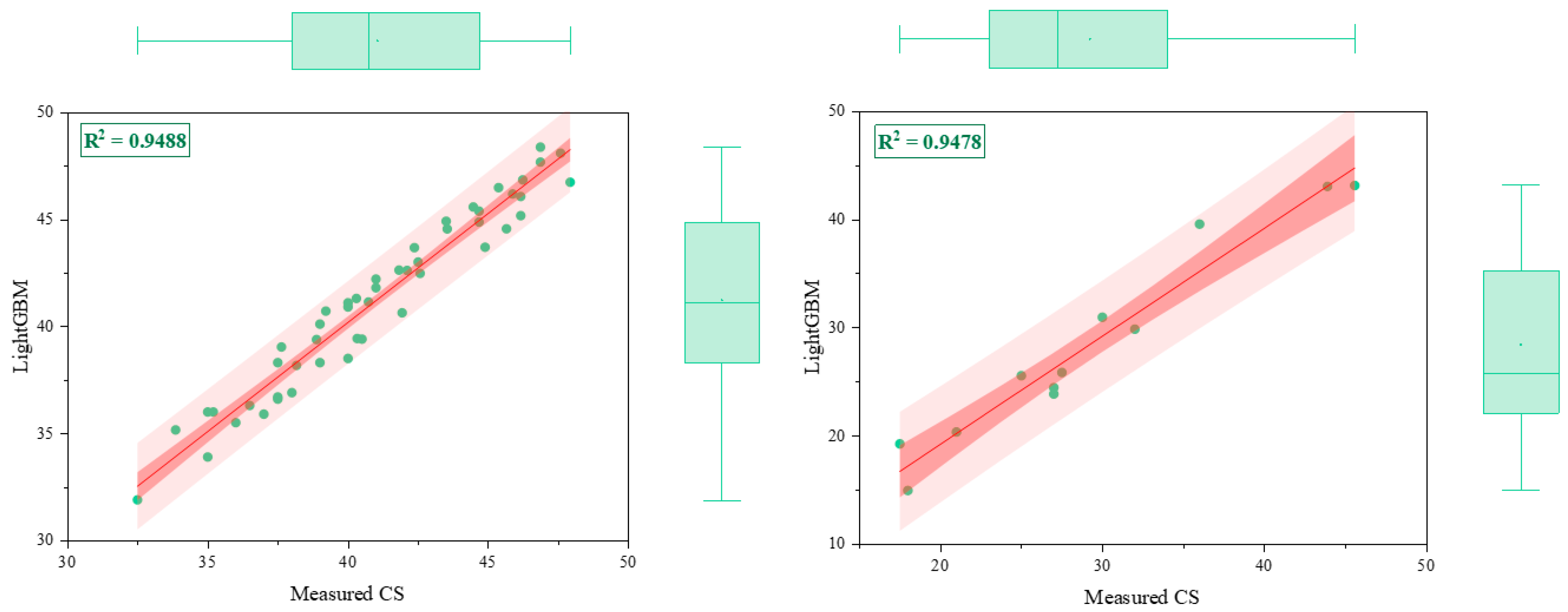
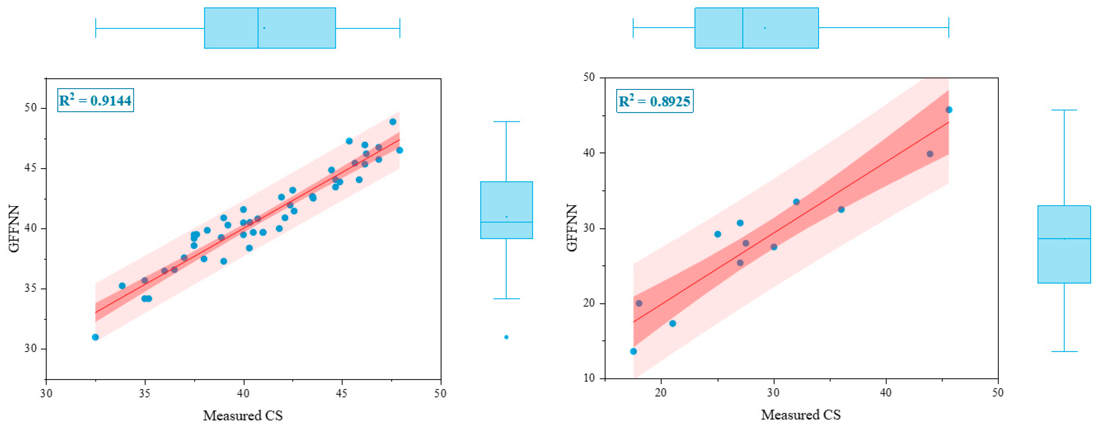
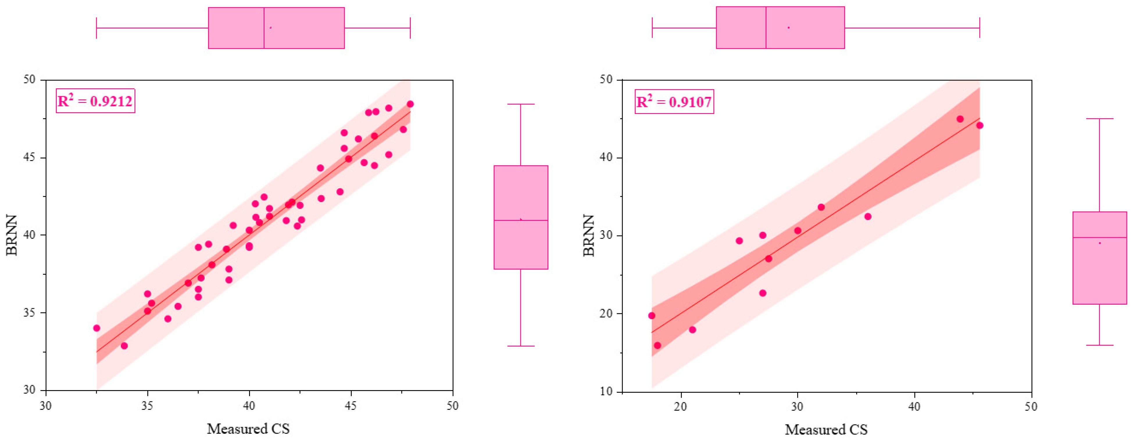
In this study, the performance of the hybrid ICA-LightGBM algorithm was evaluated in predicting CSGCo. The accuracy of this model was acceptable and can be reliably used for prediction aims. However, the accuracy of the ICA-LightGBM algorithm should be compared with the other artificial intelligence techniques so that its prediction performance can be proven. In this regard, the well-known methods were considered for evaluating ICA-LightGBM accuracy. The artificial neural networks were successfully trained in solving engineering problems. This method has different structures and architectures based on training algorithms, hidden layers, hidden neurons, and the learning rate. Therefore, we employed four main architectures involving a multi-layer perceptron neural network (MLP), radial basis function (RBF), generalized feed-forward neural network (GFFNN), and Bayesian regularized neural network (BRNN). The accuracy and performance of these models in anticipating the CSGCo were obtained. Nevertheless, their efficiency, capability, and success in predicting need to be investigated and compared. According to evaluation metrics used for ICA-LightGBM, the performance of the LightGBM, MLP, RBF, GFFNN, and BRNN was obtained and is summarized in Table 2. Furthermore, the scatter plot of the measured and the predicted values of CSGCo using ICA-LightGBM, LightGBM, MLP, RBF, GFFNN, and BRNN for both training and testing parts are demonstrated in Figure 8, Figure 9, Figure 10, Figure 11, Figure 12 and Figure 13. Based on Table 2, the LightGBM model is capable of predicting values better than MLP, RBF, GFFNN, and BRNN techniques. However, the optimized LightGBM model, i.e., ICA-LightGBM, has the most accurate results on the basis of the RMSE 0.4703 and 1.3137 for training and testing phases, respectively. As shown in Figure 8, Figure 9, Figure 10, Figure 11, Figure 12 and Figure 13 that illustrate the scatter plot of actual and estimated CSGCo in two phases of training and testing, it can be found that all the developed models estimated the CSGCo with an acceptable accuracy. However, the ICA-LightGBM model with an R2 of 0.9805 for the testing part was more accurate than the LightGBM with an R2 of 0.9478, MLP with an R2 of 0.8959, RBF with an R2 of 0.8055, BRNN with an R2 of 0.9107, and GFFNN with an R2 of 0.8925. It can be concluded that the ICA-LightGBM model is a superior model in predicting CSGCo.
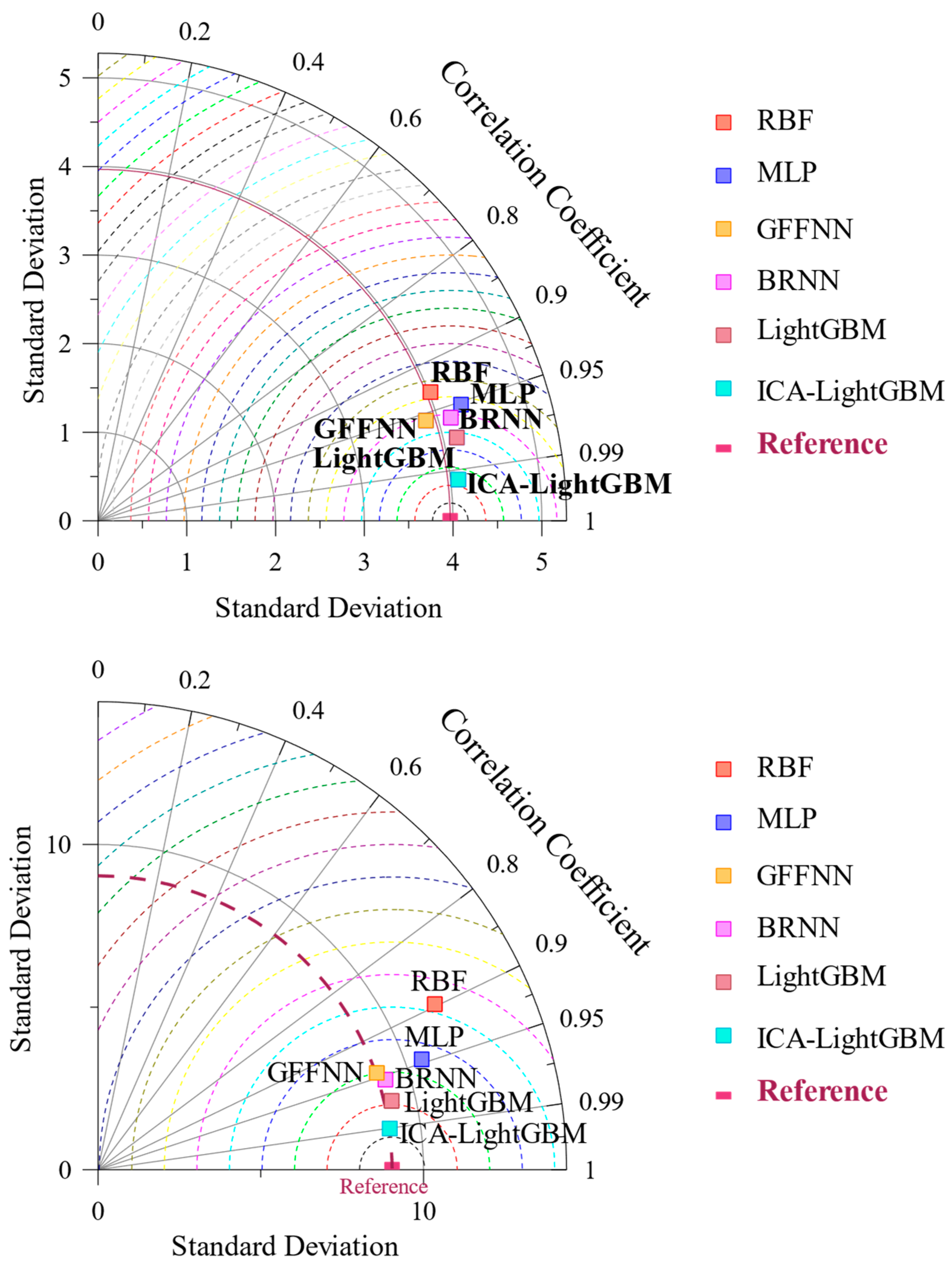
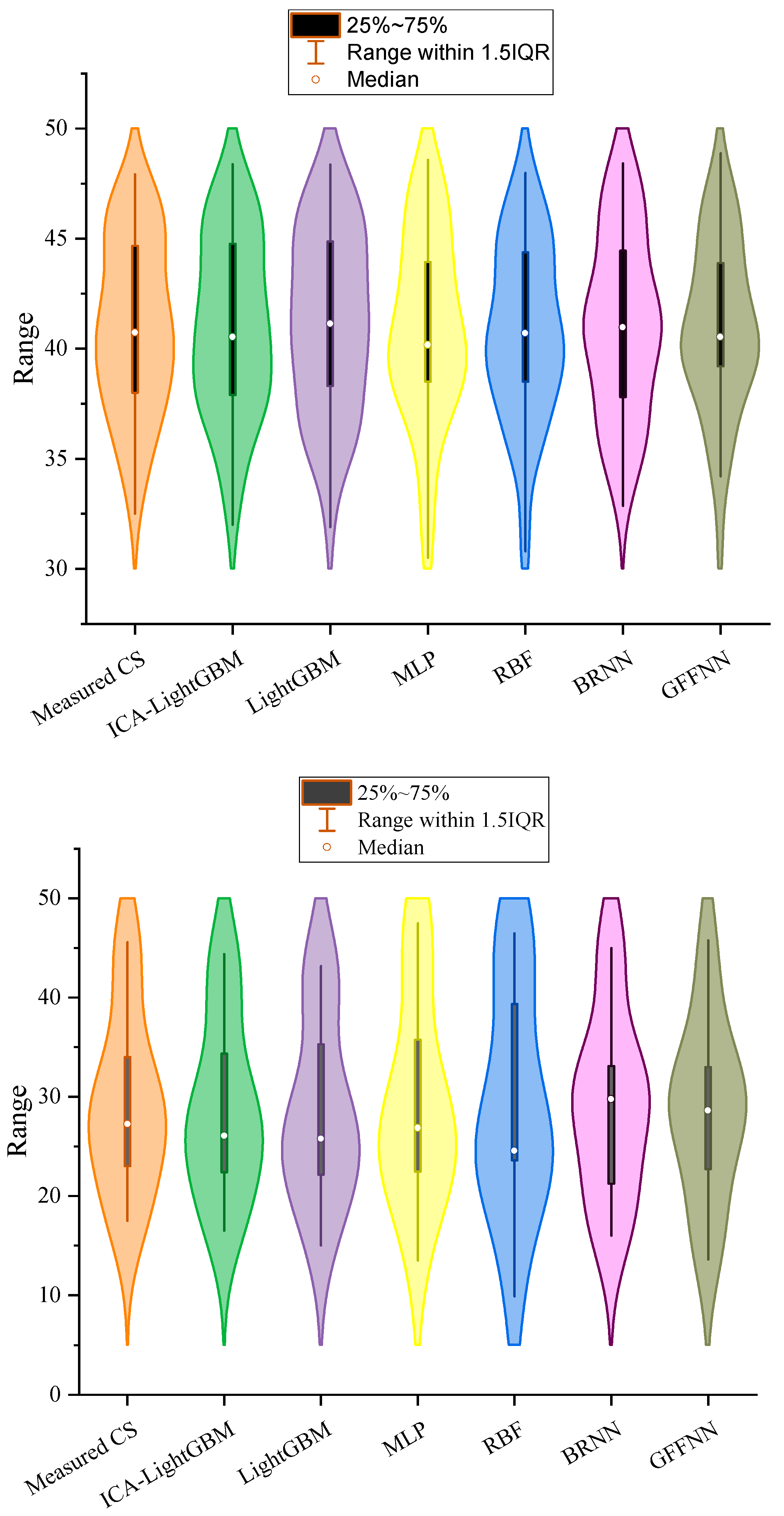
For more comparison, a Taylor diagram and Violin plot relevant to the accuracy of the models, respectively, are displayed in Figure 14 and Figure 15. From Figure 14, the ICA-LightGBM symbol was closest to reference data in both training and testing phases (measured data) and this shows that the best model is ICA-LightGBM. Furthermore, Figure 15 shows that the results of the ICA-LightGBM model are very close to the measured values.
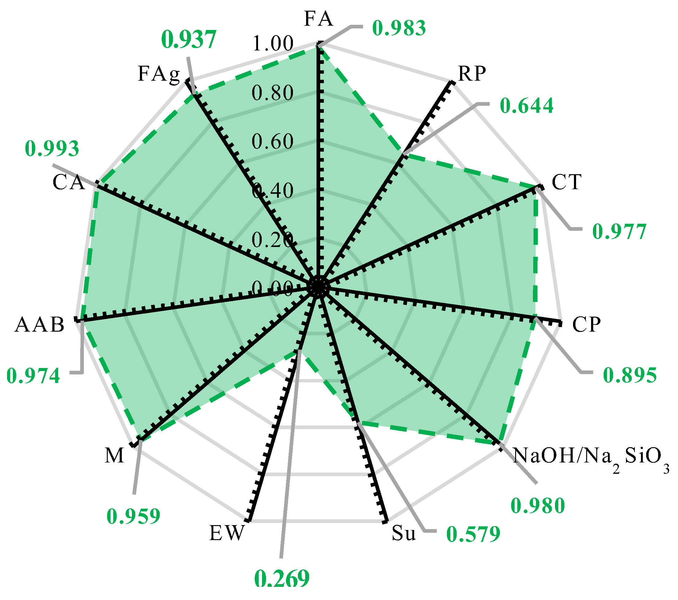
In the last step of this study, the most and least impactful parameters on determination of CSGCo were specified. To do this, a sensitivity analysis technique was employed named the Cosine Amplitude Method (CAM) [50]. The CA method measures the strength of the relationship between every two effective parameters on CSGCo. In this regard, the following equation is utilized [52]:
In which rij is the intensity impact between xi (input) and xj (output). The sensitivity results and impactful parameters were determined. From Figure 16, the CA parameter has the most effect on CSGCo with a strength of 0.993, while the least effect is related to the EW parameter with a strength of 0.269. Noteworthily, the influence of the parameters based on the rij value can be prioritized in ascending order as EW < Su < RP < CP < FAg < M < AAB < CT < NaOH/Na2SiO3 < FA < CA with an impact of 0.269, 0.579, 0.644, 0.895, 0.937, 0.959, 0.974, 0.977, 0.98, 0.983, and 0.993, respectively.
7. Conclusions
Determination and prediction of the CSGCo is a crucial issue in civil and construction fields. Hence, the accurate estimation of CSGCo can increase safety. The main contribution of the current research is to optimize hyper-parameters of the LightGBM algorithm using ICA to model the CSGCo. In addition, four various architectures of ANNs such as MLP, RBF, GFFNN, and BRNN models were applied to predict CSGCo. The inputs of all models were FA, RP, CT, CP, NaOH/Na2SiO3, Su, EW, M, AAB, CA, and FAg, while the CSGCo was considered as the target. For the training of models, 61 data samples were gathered from the literature and split into two phases of training and testing sets. The trained models were evaluated by using three statistical indicators, i.e., R2, RMSE, and VAF, and the accuracy level and performance degree of the ICA-LightGBM, LightGBM, MLP, RBF, GFFNN, and BRNN models were analyzed. The obtained results indicated that the precision of the models denoting R2 values as 0.9871, 0.9488, 0.9067, 0.8694, 0.9212, and 0.9144 for training models and 0.9805, 0.9478, 0.8959, 0.8055, 0.9107, and 0.8925 in testing models for ICA-LightGBM, LightGBM, MLP, RBF, GFFNN, and BRNN, respectively, showed a superior capability in the application of the ICA-LightGBM model in anticipating the CSGCo. It can be concluded that the ICA algorithm can be used as a powerful and robust optimizer to improve the LightGBM predictor.
Author Contributions
Conceptualization, Q.W., J.Q., S.H., H.R. and J.H.; methodology, Q.W., J.Q. and S.H.; software, Q.W., J.Q. and S.H.; validation, Q.W., J.Q., S.H., H.R. and J.H.; resources, Q.W., S.H. and J.H.; data curation, Q.W., S.H. and J.H.; writing—original draft preparation, Q.W., J.Q., S.H., H.R. and J.H.; writing—review and editing, Q.W., J.Q., S.H., H.R. and J.H.; visualization, S.H. and Q.W.; supervision, H.R., J.H. and Q.W.; funding acquisition, Q.W. and J.H. All authors have read and agreed to the published version of the manuscript.
Funding
This research received no external funding.
Data Availability Statement
The data will be available upon a request.
Conflicts of Interest
The authors declare no conflict of interest.
References
- Mahmood, A.H.; Foster, S.J.; Castel, A. Development of high-density geopolymer concrete with steel furnace slag aggregate for coastal protection structures. Constr. Build. Mater. 2020, 248, 118681. [Google Scholar] [CrossRef]
- Antony Jeyasehar, C.; Saravanan, G.; Salahuddin, M.; Thirugnanasambandam, S. Development of fly ash based geopolymer precast concrete elements. Asian J. Civ. Eng. 2013, 14, 605–615. [Google Scholar]
- Aslani, F.; Deghani, A.; Asif, Z. Development of Lightweight Rubberized Geopolymer Concrete by Using Polystyrene and Recycled Crumb-Rubber Aggregates. J. Mater. Civ. Eng. 2020, 32, 04019345. [Google Scholar] [CrossRef]
- Murthy, T.V.S.; Rai, D.A.K. Geopolymer Concrete, an Earth Friendly Concrete, Very Promisinginthe Industry. Int. J. Civ. Eng. Technol. 2014, 5, 113–122. [Google Scholar]
- Mehdizadeh, B.; Jahandari, S.; Vessalas, K.; Miraki, H.; Rasekh, H.; Samali, B. Fresh, mechanical, and durability properties of self-compacting mortar incorporating alumina nanoparticles and rice husk ash. Materials 2021, 14, 6778. [Google Scholar] [CrossRef]
- AzariJafari, H.; Amiri, M.J.T.; Ashrafian, A.; Rasekh, H.; Barforooshi, M.J.; Berenjian, J. Ternary blended cement: An eco-friendly alternative to improve resistivity of high-performance self-consolidating concrete against elevated temperature. J. Clean. Prod. 2019, 223, 575–586. [Google Scholar] [CrossRef]
- CEA (Central Electricity Authority). Fly Ash Generation at Coal/Lignite Based Thermal Power Stations and Its Utilization in the Country Report; CEA: New Delhi, India, 2015. [Google Scholar]
- Verma, M. Prediction of compressive strength of geopolymer concrete using random forest machine and deep learning. Asian J. Civ. Eng. 2023, 24, 2659–2668. [Google Scholar] [CrossRef]
- Verma, M.; Dev, N. Effect of ground granulated blast furnace slag and fly ash ratio and the curing conditions on the mechanical properties of geopolymer concrete. Struct. Concr. 2022, 23, 2015–2029. [Google Scholar] [CrossRef]
- Kumar, R.; Dev, N.; Ram, S.; Verma, M. Investigation of dry-wet cycles effect on the durability of modified rubberised concrete. Forces Mech. 2023, 10, 100168. [Google Scholar] [CrossRef]
- Borges, P.H.R.; Fonseca, L.F.; Nunes, V.A.; Panzera, T.H.; Martuscelli, C.C. Andreasen Particle Packing Method on the Development of Geopolymer Concrete for Civil Engineering. J. Mater. Civ. Eng. 2014, 26, 692–697. [Google Scholar] [CrossRef]
- Biondi, L.; Perry, M.; Vlachakis, C.; Wu, Z.; Hamilton, A.; McAlorum, J. Ambient cured fly ash geopolymer coatings for concrete. Materials 2019, 12, 923. [Google Scholar] [CrossRef] [PubMed]
- Das, S.K.; Shrivastava, S. Siliceous fly ash and blast furnace slag based geopolymer concrete under ambient temperature curing condition. Struct. Concr. 2021, 22, E341–E351. [Google Scholar] [CrossRef]
- Nath, P.; Sarker, P.K. Flexural strength and elastic modulus of ambient-cured blended low-calcium fly ash geopolymer concrete. Constr. Build. Mater. 2017, 130, 22–31. [Google Scholar] [CrossRef]
- Zannerni, G.M.; Fattah, K.P.; Al-Tamimi, A.K. Ambient-cured geopolymer concrete with single alkali activator. Sustain. Mater. Technol. 2020, 23, e00131. [Google Scholar] [CrossRef]
- Gupta, A.; Gupta, N.; Saxena, K.K. Experimental study of the mechanical and durability properties of Slag and Calcined Clay based geopolymer composite. Adv. Mater. Process. Technol. 2022, 8, 655–669. [Google Scholar] [CrossRef]
- Kumar, R.; Verma, M.; Dev, N. Investigation of fresh, mechanical, and impact resistance properties of rubberized concrete. In Proceedings of the International e-Conference on Sustainable Development & Recent Trends in Civil Engineering, Online, 4–5 January 2022; pp. 88–94. [Google Scholar]
- Kumar, R.; Verma, M.; Dev, N. Investigation on the Effect of Seawater Condition, Sulphate Attack, Acid Attack, Freeze–Thaw Condition, and Wetting–Drying on the Geopolymer Concrete. Iran. J. Sci. Technol. Trans. Civ. Eng. 2022, 46, 2823–2853. [Google Scholar] [CrossRef]
- Verma, M.; Nigam, M. Mechanical Behaviour of Self Compacting and Self Curing Concrete. Int. J. Innov. Res. Sci. Eng. Technol. 2017, 6, 14361–14366. [Google Scholar]
- Chouksey, A.; Verma, M.; Dev, N.; Rahman, I.; Upreti, K. An investigation on the effect of curing conditions on the mechanical and microstructural properties of the geopolymer concrete. Mater. Res. Express 2022, 9, 055003. [Google Scholar] [CrossRef]
- Verma, M.; Nigam, M. Experimental investigation on the properties of Geopolymer concrete after replacement of river sand with the M-sand. AIP Conf. Proc. 2023, 2721, 020029. [Google Scholar]
- Chandrasekhar Reddy, K. Investigation of Mechanical and Microstructural Properties of Fiber-Reinforced Geopolymer Concrete with GGBFS and Metakaolin: Novel Raw Material for Geopolymerisation. Silicon 2021, 13, 4565–4573. [Google Scholar] [CrossRef]
- Singh, I.; Dev, N.; Pal, S.; Visalakshi, T. Finite Element Analysis of Impact Load on Reinforced Concrete. In CIGOS 2021, Emerging Technologies and Applications for Green Infrastructure: Proceedings of the 6th International Conference on Geotechnics, Civil Engineering and Structures; Lecture Notes in Civil Engineering; Springer: Singapore, 2022. [Google Scholar]
- Cavaleri, L.; Barkhordari, M.S.; Repapis, C.C.; Armaghani, D.J.; Ulrikh, D.V.; Asteris, P.G. Convolution-based ensemble learning algorithms to estimate the bond strength of the corroded reinforced concrete. Constr. Build. Mater. 2022, 359, 129504. [Google Scholar] [CrossRef]
- Barkhordari, M.S.; Armaghani, D.J.; Mohammed, A.S.; Ulrikh, D.V. Data-Driven Compressive Strength Prediction of Fly Ash Concrete Using Ensemble Learner Algorithms. Buildings 2022, 12, 132. [Google Scholar] [CrossRef]
- Asteris, P.G.; Lourenço, P.B.; Roussis, P.C.; Adami, C.E.; Armaghani, D.J.; Cavaleri, L.; Chalioris, C.E.; Hajihassani, M.; Lemonis, M.E.; Mohammed, A.S. Revealing the nature of metakaolin-based concrete materials using artificial intelligence techniques. Constr. Build. Mater. 2022, 322, 126500. [Google Scholar] [CrossRef]
- Sarir, P.; Armaghani, D.J.; Jiang, H.; Sabri, M.M.S.; He, B.; Ulrikh, D.V. Prediction of Bearing Capacity of the Square Concrete-Filled Steel Tube Columns: An Application of Metaheuristic-Based Neural Network Models. Materials 2022, 15, 3309. [Google Scholar] [CrossRef] [PubMed]
- Biswas, R.; Bardhan, A.; Samui, P.; Rai, B.; Nayak, S.; Armaghani, D.J. Efficient soft computing techniques for the prediction of compressive strength of geopolymer concrete. Comput. Concr. 2021, 28, 221–232. [Google Scholar]
- Paji, M.K.; Gordan, B.; Biklaryan, M.; Armaghani, D.J.; Zhou, J.; Jamshidi, M. Neuro-swarm and Neuro-imperialism Techniques to Investigate the Compressive Strength of Concrete Constructed by Freshwater and Magnetic Salty Water. Measurement 2021, 182, 109720. [Google Scholar] [CrossRef]
- Sun, L.; Koopialipoor, M.; Armaghani, D.J.; Tarinejad, R.; Tahir, M.M. Applying a meta-heuristic algorithm to predict and optimize compressive strength of concrete samples. Eng. Comput. 2019, 37, 1133–1145. [Google Scholar] [CrossRef]
- Mohammed, A.; Kurda, R.; Armaghani, D.J.; Hasanipanah, M. Prediction of compressive strength of concrete modified with fly ash: Applications of neuro-swarm and neuro-imperialism models. Comput. Concr. 2021, 27, 489–512. [Google Scholar]
- Zhang, X.; Bayat, V.; Koopialipoor, M.; Armaghani, D.J.; Yong, W.; Zhou, J. Evaluation of structural safety reduction due to water penetration into a major structural crack in a large concrete project. Smart Struct. Syst. 2020, 26, 319–329. [Google Scholar]
- Liao, J.; Asteris, P.G.; Cavaleri, L.; Mohammed, A.S.; Lemonis, M.E.; Tsoukalas, M.Z.; Skentou, A.D.; Maraveas, C.; Koopialipoor, M.; Armaghani, D.J. Novel Fuzzy-Based Optimization Approaches for the Prediction of Ultimate Axial Load of Circular Concrete-Filled Steel Tubes. Buildings 2021, 11, 629. [Google Scholar] [CrossRef]
- Armaghani, D.J.; Asteris, P.G.; Fatemi, S.A.; Hasanipanah, M.; Tarinejad, R.; Rashid, A.S.A.; Huynh, V. Van On the Use of Neuro-Swarm System to Forecast the Pile Settlement. Appl. Sci. 2020, 10, 1904. [Google Scholar] [CrossRef]
- He, B.; Armaghani, D.J.; Lai, S.H. Assessment of tunnel blasting-induced overbreak: A novel metaheuristic-based random forest approach. Tunn. Undergr. Space Technol. 2023, 133, 104979. [Google Scholar] [CrossRef]
- Ghanizadeh, A.R.; Ghanizadeh, A.; Asteris, P.G.; Fakharian, P.; Armaghani, D.J. Developing Bearing Capacity Model for Geogrid-Reinforced Stone Columns Improved Soft Clay utilizing MARS-EBS Hybrid Method. Transp. Geotech. 2022, 38, 100906. [Google Scholar] [CrossRef]
- Asteris, P.G.; Rizal, F.I.M.; Koopialipoor, M.; Roussis, P.C.; Ferentinou, M.; Armaghani, D.J.; Gordan, B. Slope Stability Classification under Seismic Conditions Using Several Tree-Based Intelligent Techniques. Appl. Sci. 2022, 12, 1753. [Google Scholar] [CrossRef]
- Shan, F.; He, X.; Armaghani, D.J.; Zhang, P.; Sheng, D. Success and challenges in predicting TBM penetration rate using recurrent neural networks. Tunn. Undergr. Space Technol. 2022, 130, 104728. [Google Scholar] [CrossRef]
- Zhou, J.; Asteris, P.G.; Armaghani, D.J.; Pham, B.T. Prediction of ground vibration induced by blasting operations through the use of the Bayesian Network and random forest models. Soil Dyn. Earthq. Eng. 2020, 139, 106390. [Google Scholar] [CrossRef]
- Jahed Armaghani, D.; Ming, Y.Y.; Salih Mohammed, A.; Momeni, E.; Maizir, H. Effect of SVM Kernel Functions on Bearing Capacity Assessment of Deep Foundations. J. Soft Comput. Civ. Eng. 2023, 7, 111–128. [Google Scholar]
- Fakharian, P.; Rezazadeh Eidgahee, D.; Akbari, M.; Jahangir, H.; Ali Taeb, A. Compressive strength prediction of hollow concrete masonry blocks using artificial intelligence algorithms. Structures 2023, 47, 1790–1802. [Google Scholar] [CrossRef]
- Ke, G.; Meng, Q.; Finley, T.; Wang, T.; Chen, W.; Ma, W.; Ye, Q.; Liu, T.Y. LightGBM: A highly efficient gradient boosting decision tree. Adv. Neural Inf. Process. Syst. 2017, 30, 3147–3155. [Google Scholar]
- Wen, X.; Xie, Y.; Wu, L.; Jiang, L. Quantifying and comparing the effects of key risk factors on various types of roadway segment crashes with LightGBM and SHAP. Accid. Anal. Prev. 2021, 159, 106261. [Google Scholar] [CrossRef]
- Chen, T.; Xu, J.; Ying, H.; Chen, X.; Feng, R.; Fang, X.; Gao, H.; Wu, J. Prediction of Extubation Failure for Intensive Care Unit Patients Using Light Gradient Boosting Machine. IEEE Access 2019, 7, 150960–150968. [Google Scholar] [CrossRef]
- Atashpaz-Gargari, E.; Lucas, C. Imperialist competitive algorithm: An algorithm for optimization inspired by imperialistic competition. In Proceedings of the 2007 IEEE Congress on Evolutionary Computation, Singapore, 25–28 September 2007; IEEE: Piscataway, NJ, USA, 2007; pp. 4661–4667. [Google Scholar]
- Wang, X.; Hosseini, S.; Jahed Armaghani, D.; Tonnizam Mohamad, E. Data-Driven Optimized Artificial Neural Network Technique for Prediction of Flyrock Induced by Boulder Blasting. Mathematics 2023, 11, 2358. [Google Scholar] [CrossRef]
- Hosseini, S.; Mousavi, A.; Monjezi, M. Prediction of blast-induced dust emissions in surface mines using integration of dimensional analysis and multivariate regression analysis. Arab. J. Geosci. 2022, 15, 163. [Google Scholar] [CrossRef]
- Hosseini, S.; Poormirzaee, R.; Hajihassani, M. Application of reliability-based back-propagation causality-weighted neural networks to estimate air-overpressure due to mine blasting. Eng. Appl. Artif. Intell. 2022, 115, 105281. [Google Scholar] [CrossRef]
- Hosseini, S.; Poormirzaee, R.; Gilani, S.-O.; Jiskani, I.M. A reliability-based rock engineering system for clean blasting: Risk analysis and dust emissions forecasting. Clean Technol. Environ. Policy 2023, 25, 1903–1920. [Google Scholar] [CrossRef]
- Hosseini, S.; Poormirzaee, R.; Hajihassani, M. An uncertainty hybrid model for risk assessment and prediction of blast-induced rock mass fragmentation. Int. J. Rock Mech. Min. Sci. 2022, 160, 105250. [Google Scholar] [CrossRef]
- Hosseini, S.; Poormirzaee, R.; Hajihassani, M.; Kalatehjari, R. An ANN-Fuzzy Cognitive Map-Based Z-Number Theory to Predict Flyrock Induced by Blasting in Open-Pit Mines. Rock Mech. Rock Eng. 2022, 55, 4373–4390. [Google Scholar] [CrossRef]
- Zhao, J.; Hosseini, S.; Chen, Q.; Armaghani, D.J. Super learner ensemble model: A novel approach for predicting monthly copper price in future. Resour. Policy 2023, 85, 103903. [Google Scholar] [CrossRef]
Figure 1.
General flowchart of LightGBM model.

Figure 2.
The main hyper-parameters for controlling and optimizing LightGBM technique.

Figure 3.
(a) Generating the initial empires, (b) imperialistic competition, and (c) ICA flowchart [45].
Figure 3.
(a) Generating the initial empires, (b) imperialistic competition, and (c) ICA flowchart [45].

Figure 4.
Histogram plot and frequency of inputs and output.

Figure 5.
Heatmap of effective parameters on CSGCo.

Figure 6.
Convergence plot of the hyper-parameter optimization of the ICA-LightGBM.

Figure 7.
Comparison of predicted and measured CSGCo on the training and testing sets.


Figure 8.
Correlation of anticipated and actual CSGCo using RBF model.

Figure 9.
Correlation of anticipated and actual CSGCo using MLP model.

Figure 10.
Correlation of anticipated and actual CSGCo using LightGBM model.

Figure 11.
Correlation of anticipated and actual CSGCo using ICA-LightGBM model.

Figure 12.
Correlation of anticipated and actual CSGCo using GFFNN model.

Figure 13.
Correlation of anticipated and actual CSGCo using BRNN model.

Figure 14.
Indicating Taylor plot relevant to the developed models based on training (above) and testing (below) phases.
Figure 14.
Indicating Taylor plot relevant to the developed models based on training (above) and testing (below) phases.

Figure 15.
Violin plot of predictive models for both training (above) and testing (below) sets.

Figure 16.
The strength relationship between effective parameters on CSGCo.


Table 1.
Inputs and target of this study and their ranges.
| Type | Parameter | Sign | Unit | Min | Mean | Max | Standard Deviation |
|---|---|---|---|---|---|---|---|
| Input | Fly ash | FA | (kg/m3) | 298 | 401.92 | 430 | 39.13 |
| Rest period | RP | (h) | 0 | 14.16 | 72 | 14.78 | |
| Curing temperature | CT | (°C) | 40 | 71.80 | 100 | 18.66 | |
| Curing period | CP | (h) | 24 | 27.93 | 48 | 8.96 | |
| NaOH/Na2SiO3 | NaOH/Na2SiO3 | - | 0.3 | 0.40 | 0.5 | 0.03 | |
| Superplasticizer | Su | (kg/m3) | 0 | 4.11 | 10.5 | 4.38 | |
| Extra water added | EW | (kg/m3) | 0 | 5.74 | 35 | 13.07 | |
| Molarity | M | - | 8 | 12.66 | 18 | 2.77 | |
| Alkaline activator/binder ratio | AAB | - | 0.25 | 0.38 | 0.45 | 0.05 | |
| Coarse aggregate | CA | (kg/m3) | 875 | 1223.91 | 1377 | 158.90 | |
| Fine aggregate | FAg | (kg/m3) | 533 | 605.56 | 875 | 121.05 | |
| Target | Compressive strength | CS | (MPa) | 17.5 | 38.71 | 47.92 | 7.08 |
Table 2.
The obtained statistical metrics for evaluation of developed models.
| Evaluation Metrics | R2 | RMSE | VAF | |||
|---|---|---|---|---|---|---|
| Part | Train | Test | Train | Test | Train | Test |
| ICA-LightGBM | 0.9871 | 0.9805 | 0.4703 | 1.3137 | 98.5773 | 98.0397 |
| LightGBM | 0.9488 | 0.9478 | 0.9532 | 2.1631 | 94.3613 | 94.5173 |
| MLP | 0.9067 | 0.8959 | 1.3093 | 3.3648 | 88.9888 | 84.9125 |
| RBF | 0.8694 | 0.8055 | 1.4703 | 5.0309 | 86.3122 | 66.1888 |
| BRNN | 0.9212 | 0.9107 | 1.1510 | 2.6569 | 91.4168 | 90.5854 |
| GFFNN | 0.9144 | 0.8925 | 1.1525 | 2.9415 | 91.4092 | 88.9088 |
Disclaimer/Publisher’s Note: The statements, opinions and data contained in all publications are solely those of the individual author(s) and contributor(s) and not of MDPI and/or the editor(s). MDPI and/or the editor(s) disclaim responsibility for any injury to people or property resulting from any ideas, methods, instructions or products referred to in the content. |
© 2023 by the authors. Licensee MDPI, Basel, Switzerland. This article is an open access article distributed under the terms and conditions of the Creative Commons Attribution (CC BY) license (https://creativecommons.org/licenses/by/4.0/).
Share and Cite
MDPI and ACS Style
Wang, Q.; Qi, J.; Hosseini, S.; Rasekh, H.; Huang, J. ICA-LightGBM Algorithm for Predicting Compressive Strength of Geo-Polymer Concrete. Buildings 2023, 13, 2278. https://0-doi-org.brum.beds.ac.uk/10.3390/buildings13092278
AMA Style
Wang Q, Qi J, Hosseini S, Rasekh H, Huang J. ICA-LightGBM Algorithm for Predicting Compressive Strength of Geo-Polymer Concrete. Buildings. 2023; 13(9):2278. https://0-doi-org.brum.beds.ac.uk/10.3390/buildings13092278
Chicago/Turabian StyleWang, Qiang, Jiali Qi, Shahab Hosseini, Haleh Rasekh, and Jiandong Huang. 2023. "ICA-LightGBM Algorithm for Predicting Compressive Strength of Geo-Polymer Concrete" Buildings 13, no. 9: 2278. https://0-doi-org.brum.beds.ac.uk/10.3390/buildings13092278
Note that from the first issue of 2016, this journal uses article numbers instead of page numbers. See further details here.