Dynamic Modeling of Heat Exchangers Based on Mechanism and Reinforcement Learning Synergy

1
School of Civil Engineering, Inner Mongolia University of Technology, Hohhot 010051, China
2
School of Energy and Power Engineering, Inner Mongolia University of Technology, Hohhot 010080, China
3
National Carbon Measurement Center (Inner Mongolia), Hohhot 010050, China
*
Author to whom correspondence should be addressed.
Buildings 2024, 14(3), 833; https://0-doi-org.brum.beds.ac.uk/10.3390/buildings14030833
Submission received: 7 February 2024
/
Revised: 9 March 2024
/
Accepted: 16 March 2024
/
Published: 20 March 2024
(This article belongs to the Section Building Energy, Physics, Environment, and Systems)
Abstract
:The current lack of a high-precision, real-time model applicable to the control optimization process of heat exchange systems, especially the difficulty in determining the overall heat transfer coefficient K of heat exchanger operating parameters in real time, is a prominent issue. This paper mainly unfolds the following work: 1. We propose a dynamic model for the control and optimization of the heat exchanger operation. By constructing a system to collect real-time operating data on the flow rates and temperatures on both sides of the heat exchanger, the parameter identification of the overall heat transfer coefficient K is performed. Subsequently, by combining this with mechanistic equations, a novel heat exchanger model is established based on the fusion of mechanistic principles and reinforcement learning. 2. We validate the new model, where the average relative error between the model’s temperature output values and the actual measured values is below 5%, indicating the high identification accuracy of the model. Moreover, under variations in the temperature and flow rate, the overall heat transfer coefficient K demonstrates the correct patterns of change. 3. To further enhance the model’s identification accuracy, a study on the reward functions in reinforcement learning is conducted. A model with the Logarithmic Mean Temperature Difference (LMTD) as the reward function exhibits a high identification accuracy. However, upon comparison, a model using the Arithmetic Mean Temperature Difference (AMTD) for relative error as the reward function shows an even higher identification accuracy. The model is validated under various operating conditions, such as changes in the flow rate on the hot side, demonstrating good scalability and applicability. This research contributes to providing a high-precision dynamic parameter basis for the precise control of heat exchange systems, offering significant guidance for the control optimization of actual heat exchange system operations.
1. Introduction
Heating, ventilation, and air conditioning (HVAC) systems are widely employed in the field of construction. Research from the International Energy Agency (IEA) indicates that the total energy consumption in the global construction sector constitutes approximately 40% of the overall energy consumption [1]. HVAC systems, in turn, contribute to 40–50% of the total energy consumption in buildings [2]. The operational efficiency of a heating system is particularly crucial for reducing its energy consumption [3]. Chen et al. [4] specifically designed the heat transfer performance of a gradient thickness TPMS heat exchanger, achieving a 4.2% improvement in the overall heat transfer efficiency through systematic design. Samer Ali et al. [5] introduced an innovative algorithm for the heat transfer coefficient in heat exchangers, significantly aiding in the precision enhancement of energy-efficient designs for heat exchangers, and consequently, improving the operational efficiencies of heat exchange systems. The rapid development of Internet of Things (IoT) technology has significantly contributed to the improvement in the operational efficiency. Li, W.-T. et al. [6] employed the IoT to formulate control strategies, enhancing the operational efficiencies of solar water heating systems (SWHs) and substantially reducing the operational costs associated with SWHs. Li et al. [7] employed a model predictive control method distinct from traditional control approaches for district heating (DH) regulation. This approach led to an improvement in the operational efficiency of DH, resulting in a 7.4% reduction in system energy consumption. The popularity of reinforcement learning has also contributed to the development of systems with an improved operational efficiency. Zhuang et al. [8] utilized the Internet of Things (IoT) and reinforcement learning to enhance the operations of heating, ventilation, and air conditioning (HVAC) systems. This approach resulted in energy savings of 17.4%, accompanied by a significant improvement in the operational efficiency. Jiang et al. [9] applied reinforcement learning techniques for the optimization of control strategies in HVAC systems. The enhanced operational efficiency led to a 6% reduction in the operating costs, underscoring the crucial importance of improving the operational efficiency of heating systems.
To ensure the efficient operation of the heat exchange system, it is imperative to enhance the precision of internal dynamic parameters within the system. Achieving this precision involves the dynamic modeling of the heat exchange system, particularly concerning the accurate representation of its internal parameters. Numerous scholars have conducted research on dynamic simulation modeling of heat exchangers. One approach involves modeling based on mechanistic equations [10], utilizing mathematical equations to describe the internal heat transfer processes within the heat exchanger. Gao et al. [11] established a novel finned-tube heat exchanger, introducing radiation heat transfer coefficients and radiative heat absorption coefficients to obtain a new mathematical model. This method, based on physical and thermodynamic principles, seeks to accurately predict the system’s performance by constructing a mathematical model of the heat exchanger. The significance of mechanistic equation modeling lies in providing a profound understanding of the internal heat transfer mechanisms within the system. It is characterized by a high precision and strong physical interpretability. However, it comes with a high complexity, and modeling complex systems using this approach may encounter limitations. Another approach involves modeling based on a large amount of actual operational data [12], utilizing statistical and data analysis techniques to establish mathematical models through data fitting. Cao [13] employed a data-driven approach to modeling, addressing issues related to low data quality. This method places a greater emphasis on acquiring system performance data through actual observations, making it widely applicable and relatively straightforward. However, its accuracy is highly dependent on the data quality, and it may result in a relatively limited understanding of the internal mechanisms of the system. Some researchers have proposed a combined approach of utilizing both the mechanisms and data to establish heat exchanger models. Zhong et al. [14] developed a thermodynamic gray-box model to analyze the coupled characteristics of a self-circulating radiator and an air-source heat pump. This gray-box model was established through a combination of mechanistic and data-driven approaches. Lu [15], similarly, proposed a method for identifying the parameters of a heating system model based on the least squares approach, combining mechanistic modeling and historical operational data. In this approach, they primarily utilize historical operational data, which does not ensure real-time information about the system’s current operation. Therefore, to achieve a precise and real-time description of the heat transfer parameters in the heat exchanger process [16], this paper proposes a modeling approach for heat exchangers driven by a synergy of the mechanisms and data. The main part of the heat exchanger model utilizes mathematical equations based on the principles of heat transfer. Another component employs real-time operational data for the simultaneous identification of the heat transfer parameters. This approach ensures the accuracy of the heat exchanger model while simultaneously guaranteeing the real-time nature of the identified heat transfer parameters. However, the most crucial aspect of an accurate heat exchanger model lies in the identification of the dynamic parameters reflecting the heat transfer performance within the heat exchanger.
Parameter identification technology is a technique that combines theoretical models with the operational data for prediction, and there are various methods for parameter identification. Parameter identification can be categorized into traditional parameter identification algorithms and intelligent parameter identification algorithms. The least squares algorithm, a traditional parameter identification method, is the most fundamental and widely applied approach in the field of system parameter identification. However, it is limited to the identification of parameters for linear, steady-state systems. Miao et al. [17] utilized a gray-box model to establish the identification of outlet temperatures in a plate heat exchanger. Dong et al. [18] employed a small amount of heat exchanger performance test data and accurately determined the model coefficients using the least squares method embedded in MATLAB. This allowed them to obtain the heat transfer efficiency surface. This identification, based on historical data, lacks real-time capabilities. Zhao et al. [19] proposed a method for online parameter identification using a least squares recursive algorithm, enabling real-time, online identification for the diagnosis of abnormal leakage conditions in heat exchangers. Intelligent parameter identification methods include neural networks [20,21], particle swarm algorithms [22], genetic algorithms (GA) [23], and reinforcement learning (RL) technology. Wang et al. [24] utilized a Radial Basis Function (RBF) neural network to establish quantitative relationships between system input variables and model parameters, enabling the identification of unknown parameters and obtaining a relatively accurate model for the heat exchange energy-saving system. Wan et al. [25] employed genetic algorithms to identify the thermal circuit model, effectively overcoming the challenges associated with determining the equivalent thermal circuit parameters for power devices. Francesco M. Solinas et al. [26] compared three different reinforcement learning methods for optimizing heating, ventilation, and air conditioning (HVAC) systems. The results, compared with simulation software like Energy Plus 23.2.0, indicated that the proposed approach based on online and imitation learning could provide reliable and cost-effective solutions for HVAC optimization problems. Therefore, reinforcement learning techniques have made significant progress in their application to parameter identification.
This paper focuses on plate heat exchangers in building heating systems and proposes a novel heat exchanger model based on the synergy of mechanism- and data-driven approaches. The aim is to achieve real-time dynamic parameter identification for precise control in the heating system. Based on the new heat exchanger model, a method for identifying the real-time dynamic parameter values within the heat exchanger using reinforcement learning techniques is proposed by the authors. Different reinforcement learning reward functions are introduced to enhance the model’s identification accuracy. Through this approach, the accuracy and applicability of the new heat exchanger model are validated. Various sets of actual operational data are employed in the system to verify the interpretability and physical relevance of the model.
2. Methodology
2.1. Overview
The research methodology consists of three parts: first, the establishment of a new heat exchanger model based on a combination of mechanistic equations and operational data; second, the collection of real-time operational data for the heat exchanger; and third, parameter identification based on reinforcement learning techniques. This paper aims to create a novel heat exchanger model by integrating mechanistic equations with operational data and utilizing reinforcement learning to identify the parameters, particularly the total heat transfer coefficient (K). For the model based on the synergistic drive of mechanistic equations and operational data in heat exchanger modeling, there are three main components: operational data, reinforcement learning, and mechanistic equations. The process begins by collecting data to obtain the real-time values of the Logarithmic Mean Temperature Difference (LMTD) from the inlet and outlet temperatures and flow rates on both sides of the heat exchanger. Next, a portion of the operational data, specifically the inlet temperatures and flow rates on both sides of the heat exchanger, is incorporated into the mechanistic equations. Additionally, the reinforcement learning approach is employed to train and obtain the overall heat transfer coefficient (K) values. This integration allows for the identification of LMTD values. At this stage, the reinforcement learning agent evaluates the relative error between the real-time LMTD values and identified LMTD values, using it as a reward function. Actions that satisfy the reward function conditions, such as specific values of K, are then output as the identified K values. This completes the establishment of the new model.
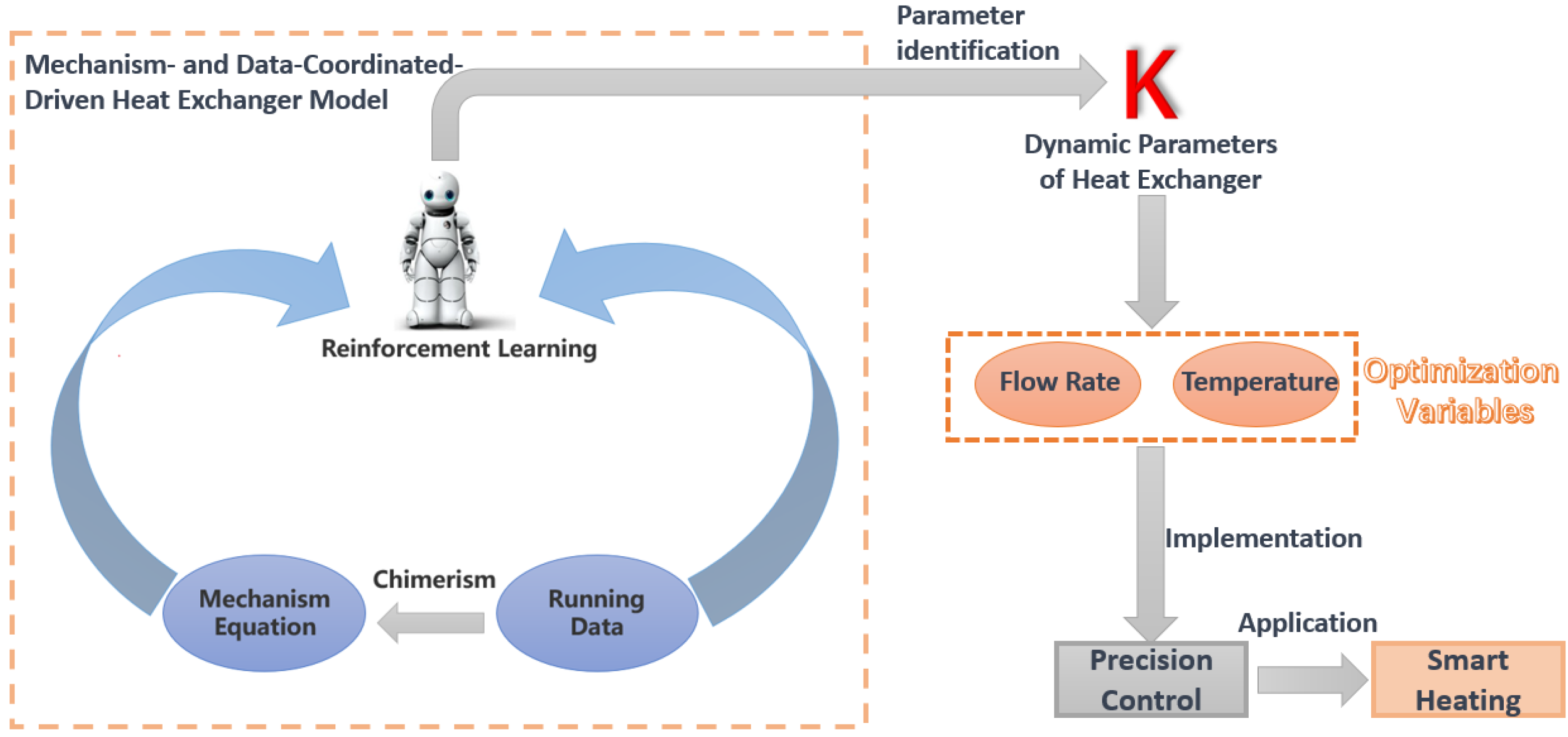
The framework, as illustrated in Figure 1, involves combining the temperature, flow rates, and other operational data with mechanistic equations primarily based on heat transfer principles. The application of reinforcement learning facilitates the identification of the total heat transfer coefficient (K) by integrating the mechanistic equations with the operational data, resulting in the formation of a new heat exchanger model. The identified K value is then utilized to regulate the flow rates and temperatures, enabling precise control and meeting the requirements of modern construction for intelligent heating.
2.2. Heat Exchanger Modeling Method
Plate heat exchangers, as one of the most widely used types of heat exchangers, operate based on the principles of heat transfer and convective heat exchange. In these systems, high-energy hot fluids and low-energy cold fluids undergo non-contact heat exchange. The high-energy hot fluid loses heat energy through the exchange process, while the low-energy cold fluid gains heat energy. The heat exchange quantity, which represents the heat produced by the heat exchange system, can be expressed as:
represents the heat generated by the heat exchange system; is the total heat transfer coefficient of the heat exchanger; is the heat transfer area; and is the temperature difference between the hot and cold fluids. ∆t represents the temperature difference between the two fluids on both sides of the heat exchanger. Introducing the concept of Logarithmic Mean Temperature Difference (LMTD) within the framework of energy conservation, the equation for LMTD is given by:
and represent the temperatures of the input and output fluids on the hot side of the heat exchanger, while and represent the temperatures of the input and output fluids on the cold side of the heat exchanger. Combining Equations (1) and (2), the expression is given by:
Similarly, the heat Q can be described using the heat transfer equation:
When the states of the cold and hot fluids are known, K or Q can be calculated through Equation (3). In practical heating operations, the controllable state variables are only and . To achieve a more detailed and transparent heat transfer process, the heat transfer effectiveness U is introduced, and the equation is given by:
NTU (Number of Transfer Units) is the number of heat transfer units, representing the fundamental unit of the heat transfer process in the heat exchanger. is the ratio of the minimum heat capacity to the maximum heat capacity in the cold and hot fluids. The equations for NTU and are given by:
The plate heat exchanger consists of cold fluid and hot fluid. Starting from the basic equations of energy conservation and mass conservation, the relationship between the heat capacity and mass flow rates of the hot and cold fluids is considered:
and are the specific heat capacities of the hot and cold fluids, respectively. and represent the heat capacities of the hot and cold fluids, respectively. Equations (10) and (11) provide the basic physical properties of the hot and cold fluids. Equation (7) imposes constraints on the design of the heat exchanger and offers valuable information for analyzing its heat transfer performance. Combining these equations completes the mechanistic modeling of the heat exchanger, ensuring stability and precision. Additionally, it allows for the solution of indirectly observed state variables. The value of K in Equation (1) is an indirectly observed state variable. To construct a new heat exchanger model, real-time and accurate values of K are required. The use of reinforcement learning facilitates the parameter identification of K, leading to the formation of the new heat exchanger model. The application of reinforcement learning relies on the support of operational data for training and learning, necessitating the collection of such data.
2.3. Heat Exchanger Real-Time Operation Data Collection
2.3.1. Heat Exchanger System Description
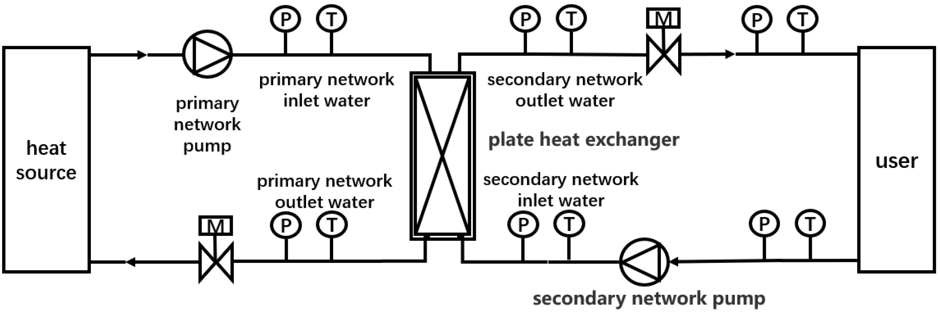
The application scenario of the heat exchanger is based on the operation of a traditional heat exchange system, and the schematic diagram of the heat exchange system is illustrated in Figure 2. The heat exchanger is a crucial component of the heat exchange system, serving as the heat exchange unit for the primary and secondary networks. The heat exchanger adopts a liquid-to-liquid plate heat exchanger, specifically choosing the counter-current flow design. The two liquids, cold and hot, achieve intermittent heat transfer through the regularly arranged corrugated channels on the heat exchange plates, accomplishing the goal of heat exchange. The heat source provides high-temperature water, which enters the heat exchanger through the primary side inlet. Simultaneously, low-temperature water from the secondary side enters the heat exchanger through the secondary side inlet. Heat exchange occurs between the high-temperature water from the primary side and the low-temperature water from the secondary side through the plate heat exchanger. The high-temperature water from the primary side, after undergoing heat exchange and becoming low-temperature water, re-enters the heat source for reheating. The low-temperature water from the secondary side, having undergone heat exchange and become high-temperature water, enters the user end for heat dissipation. This forms a cyclic process, constituting the heat exchange system.
2.3.2. Heat Exchange System Setup
The heat exchange system mainly includes equipment such as the primary heat source, electromagnetic valves, flow meters, temperature sensors, plate heat exchangers, primary network pump, and secondary network pump, with the main parameters and accuracy of the system set up as shown in Table 1. On both sides of the heat exchanger are the cold fluid and hot fluid, both consisting of water. The heat source is formed by a heater with a certain power heating the hot water tank. The known boundaries are set as the cold fluid inlet temperature, hot fluid inlet temperature, cold fluid flow rate, and hot fluid flow rate. The inlet temperatures are measured using temperature sensors, and the fluid flow rates are measured using flow meters, with flow regulation performed using a primary network pump.
2.3.3. Data Preprocessing
The heat exchange system generates a considerable volume of operational data, often containing numerous outliers and missing values. To improve the quality of the raw data, it is essential to preprocess the data through data cleaning. For outlier detection, a univariate outlier identification method is employed. The main approach involves observing the distribution of the target variable itself and using statistical methods to identify samples with a low probability, indicating anomalies. In this paper, the 2-sigma method is employed for the outlier data. This is a statistical method used to assess whether data deviates from the normal range. In this approach, under normal circumstances, 68% of the data should fall within one standard deviation from the mean, and 95% should be within two standard deviations. By calculating the mean and standard deviation of the data, it is possible to identify which values deviate from the normal range. Once the outliers are identified, options include deleting them, replacing them with the mean, or using other interpolation methods. Eliminating outliers helps maintain the consistency and accuracy of the data. First, the mean and standard deviation of the variable are calculated, and then the upper and lower limits for outliers are determined based on the formula, allowing for the identification of abnormal samples.
The upper and lower limit formulas for outlier values are as follows:
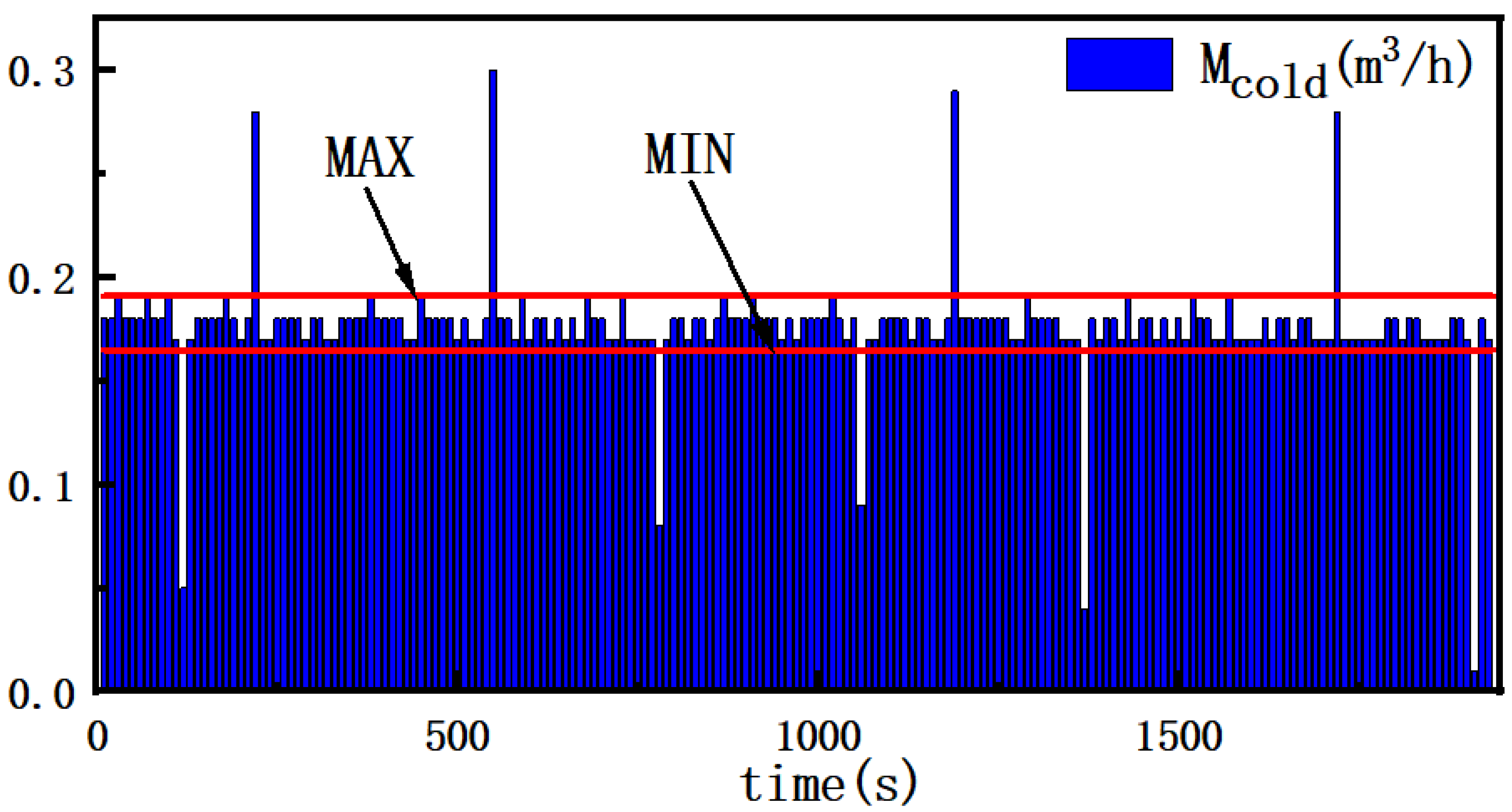
represents the mean; and represents the standard deviation. The processing of outlier values is illustrated using the 2-sigma method for the cold-side flow rate of data set one. As shown in Figure 3, the upper and lower limits are determined based on the formula, and the data outside these limits are identified as outliers and subsequently removed, thus completing the preprocessing of outlier values.
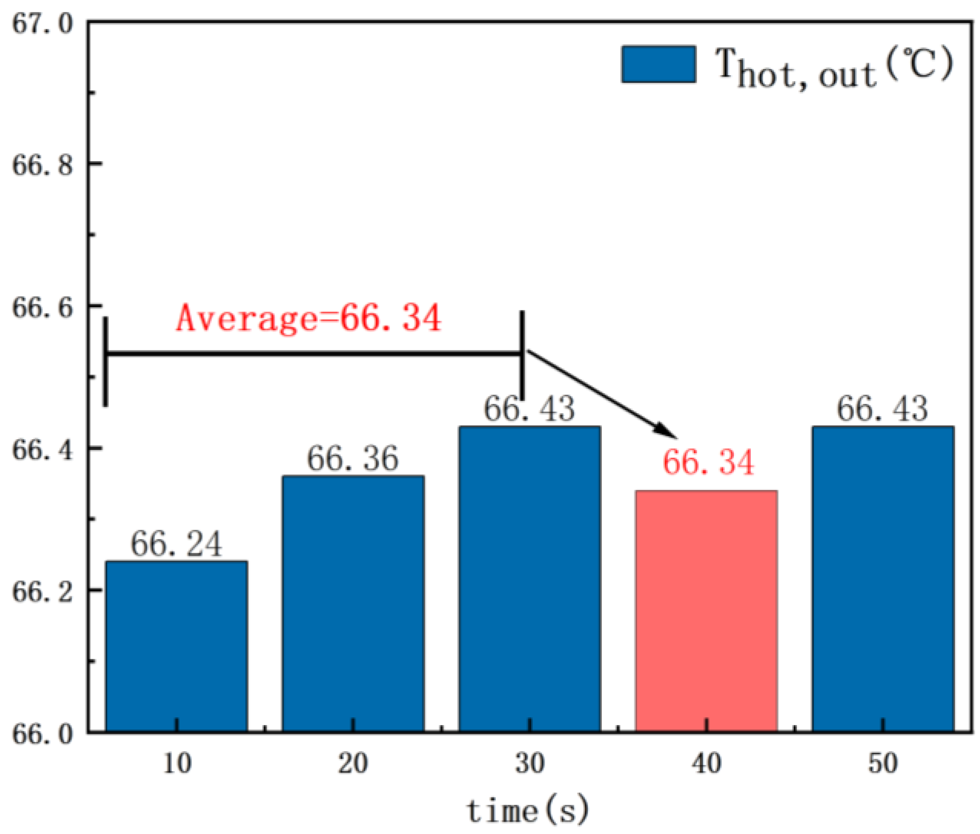
In thermal exchange systems, sensors may experience data loss due to various reasons, such as sensor malfunctions, communication failures, or other technical issues resulting in partially missing data. In such situations, it is necessary to employ suitable methods to impute or handle the missing continuous values, ensuring the continuity and availability of the data. For missing values, the moving average method is employed for imputation. Since operational data represent continuous values of the heat exchange system over consecutive time intervals, exhibiting a strong continuity and dynamic patterns, the core idea of the moving average method is that the value of a variable at a specific moment is close to its values in the adjacent time segment. To fill a missing value, the average of the three data points before the missing one is used, ensuring the continuity of the data. To handle missing values, the exit temperature on the hot flow side is taken as an example, as shown in Figure 4. At 40 s, there was a missing value in the outlet temperature. The missing value was imputed by taking the average of the preceding three outlet temperatures at that time, completing the preprocessing of the missing values. This approach maximizes the improvement of the temperature at the missing point, minimizing the loss of data quality.
The author selected two sets of data that underwent changes in two operating conditions for preprocessing. Dataset 1 involved a change in the hot fluid flow rate from 0.79 m3/h to 0.69 m3/h and a cold fluid flow rate of 0.18 m3/h. The data collection period included the period before and after the flow rate change, resulting in a total of 184 data points. Among them, there were 5 missing values and 9 outliers. The outliers were removed, and the missing values were filled using the moving average method, resulting in a final dataset of 184 data points. Dataset 2 involved a change in the hot fluid flow rate from 0.69 m3/h to 0.93 m3/h and a cold fluid flow rate of 0.18 m3/h. The total number of data points was 434, with 11 missing values and 20 outliers. After data cleaning, the final dataset consisted of 434 data points.
2.4. Parameter Identification Using Reinforcement Learning
2.4.1. Reinforcement Learning Process
The key components of reinforcement learning are the intelligent agent, environment, state, action, and reward. During the process of parameter identification for the overall heat transfer coefficient K, the dynamic parameters of K are considered as the actions of the intelligent agent. The heat exchanger unit serves as the environment, and key state parameters from the mechanistic model are treated as the state variables. The relative error between the model output and experimental output for the Logarithmic Mean Temperature Difference (LMTD) is utilized to construct the reward function, where smaller relative errors result in higher rewards. The choice of using temperature differences in the reward function will be explained in subsequent sections. The Deep Deterministic Policy Gradient (DDPG) algorithm [27] is employed for the parameter identification process. This allows for the real-time overall heat transfer coefficient K under the system operation to be obtained by utilizing the LMTD output from the reinforcement learning approach. Thus, the construction of the heat exchanger model based on the collaboration between mechanistic equations and operational data is completed. The reinforcement learning process is illustrated in Figure 5.
Reinforcement learning is a data-driven training and processing approach. The reinforcement learning system we built relies on the Python language and is developed in the PyCharm environment. The agent serves as the brain of reinforcement learning, responsible for recording the state variables, receiving real-time reward information, and adjusting its actions. Through these processes, the agent interacts with the environment. The environment setup includes describing the mechanistic equations and importing the operational data, creating an environment specific to the heat exchanger. The environment provides feedback to the agent on the current state variables (temperature and flow rate). The agent evaluates the process through a reward function, storing states and actions that satisfy the reward function and receiving corresponding immediate rewards. To meet the criteria, the agent adjusts the actions, re-enters the environment, and continues the learning process until all operational conditions in the running data are learned. Once all conditions meet the reward function, the agent outputs all identified values of K and the maximum cumulative reward value, completing the identification of the overall heat transfer coefficient K. The overall heat transfer coefficient K is a non-directly observable state variable in heat transfer parameters and is influenced by various factors. The use of reinforcement learning technology for parameter identification can effectively address the issue of dynamically uncertain parameters, especially for physically unobservable state quantities. This application extends the scope of dynamic parameter identification work to various fields.
The reward is calculated through a reward function, and its core is that if the action results in a smaller error, the reward for that action will be larger. If an action exploration does not receive a reward, it indicates that the action produces results higher than the set error’s lower limit, and the agent will continue to explore action values that satisfy the reward. The specific reward function equation is described as follows:
represents the accumulated reward value, and represents the relative error between the model output and the data output of the LMTD. The reward values are assigned as follows: if the relative error is less than 15%, the reward value is 1; if the relative error is less than 10%, the reward value is 5; if the relative error is less than 5%, the reward value is 10. The magnitude of the reward value primarily depends on the design of the reward function. However, the selection of action values for different operating conditions also has some impact on the heat exchanger. Therefore, tuning before applying reinforcement learning for parameter identification is crucial. According to the research experience of this paper, tuning the hyperparameters not only affects the exploration of high reward values but also influences the efficiency of exploring high reward values. For instance, when setting the range of action K, this study selected a set of operating data from the database for identification. Since the system operation is a dynamic process, it is not possible to directly calculate the real-time value of K based on the mechanistic equation. Instead, it can be assumed that all state variables at a certain moment take on steady-state values, thereby calculating a reference value for K. This calculated value cannot be used as a standard for comparing K but only serves as a reference for selecting the action range. Firstly, the data should be observed, and then, based on Formulas (3) and (4), the maximum and minimum values corresponding to the observed data can be identified. In these two transient states, the maximum instantaneous K value and the minimum instantaneous K value can be obtained. Based on this, the range of parameter identification action values can be selected, providing strong support for the efficiency and accuracy of the identification.
2.4.2. Markov Decision Process
The fundamental framework of reinforcement learning is the Markov Decision Process (MDP) [28], used to simulate the stochastic policy and rewards achievable by an agent in an environment where the system state exhibits the Markov property. The essence of Markov refers to the fact that the next state of a system model depends only on the current state and is independent of earlier states. This is also the main reason for identifying the parameters of the total heat transfer coefficient K for the heat exchanger. By utilizing the Markov Decision Process, the next action K can be determined based on various directly observable heat exchange state variables of the current heat exchanger. This helps in judging how the action K changes, thereby determining all the state variables and actions in the next state, independent of the previous state. This process completes real-time training on operational data and can be defined as follows:
represents the state transition probability, denotes the system state, and t represents the moment in time.
In the Markov Decision Process (MDP), a policy is the probability distribution of an agent choosing actions at each state. Due to the uncertainty of the environment, the agent may opt for a random policy, meaning it selects different actions with varying probabilities in the same state. This helps strike a balance between exploration and exploitation, enabling the agent to better understand the environment and gain more rewards. The agent obtains rewards through interactions with the environment. A reward is a numerical value representing the goodness or badness of the agent’s current action. The combination of a random policy and rewards allows the agent to adjust its strategy based on the received rewards, aiming to maximize the cumulative rewards. In reinforcement learning, the agent learns and trains on the operating data using a random policy and implemented rewards, with the MDP providing the fundamental structure for the operating data.
The key assumption of the MDP is the Markov property, which states that given the current state and action, the future state depends only on the current state and action, independent of the previous states and action sequence. The MDP is used to model and solve reinforcement learning problems, where an agent learns and optimizes its strategy to maximize long-term rewards. Various reinforcement learning algorithms, such as Q-learning and deep reinforcement learning, operate within the MDP framework. Similarly, the DDPG algorithm chosen in this study is also based on the MDP framework.
2.4.3. The Deep Deterministic Policy Gradient (DDPG) Algorithm
Reinforcement learning techniques that can be applied for dynamic parameter identification of heat exchangers include algorithms such as Q-Learning [29], Deep Q Network [30], Actor–Critic [31], etc. Dynamic parameter identification of heat exchangers involves continuous parameter adjustment requirements, forming a high-dimensional state space with multiple state variables. Moreover, the heat exchanger is part of a nonlinear and highly complex system. Therefore, this paper opts for the DDPG algorithm.
The DDPG (Deep Deterministic Policy Gradient) is a reinforcement learning algorithm that falls within the realm of deep reinforcement learning. It is designed to address problems in continuous action spaces, combining policy gradient methods with deep learning techniques. DDPG is effective in learning and optimizing deterministic policies. The DDPG algorithm was introduced by Lillicrap et al. [32] to address problems involving continuous action control. It incorporates an Actor–Critic structure and an experience replay mechanism to enhance its performance; Gu et al. [33] improved the DDPG algorithm by proposing a method that combines the use of a model to enhance the sample efficiency in real-world environments; Haarnoja et al. [34] further introduced the Soft Actor–Critic (SAC) algorithm, building upon the DDPG and incorporating the maximum entropy theory to enhance its robustness to randomness; Fujimoto et al. [35] reviewed the development of the DDPG and proposed a method to address function approximation errors, aiming to further enhance the algorithm’s performance.
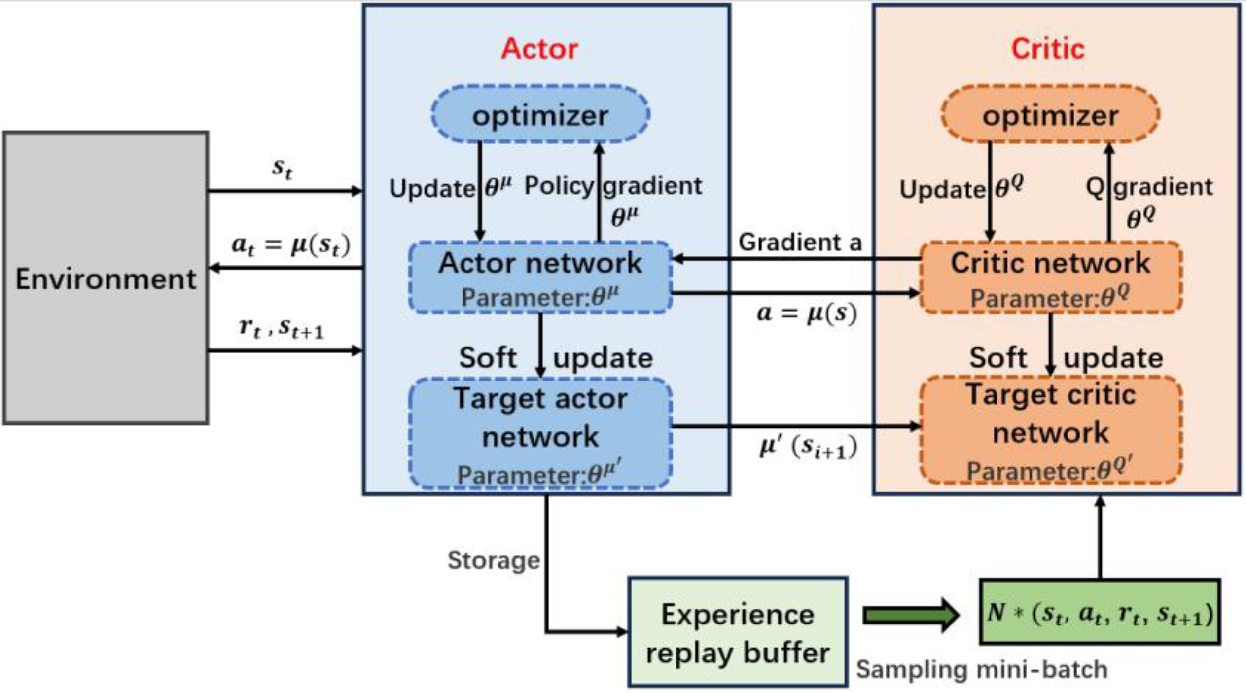
The DDPG algorithm consists of five components: the actor network, the critic network, an experience replay buffer, target actor network, and target critic network. The algorithm framework is illustrated in Figure 6.
The actor network is responsible for outputting the actions that should be taken given a certain state. The input to the policy network consists of various directly observable state variables in the current heat exchange system, such as parameters like the inlet temperature and flow rate of the hot fluid, the inlet temperature and flow rate of the cold fluid, etc. The output is the selection of the corresponding action K within the specified action range. Specifically, the policy network is represented by a deep neural network, typically with parameters, comprising fully connected layers and activation functions. The activation function of the output layer is typically the tanh function, ensuring that the output lies within the range of the continuous action space. The critic network is used to estimate the state value of performing a certain action, and this network helps the policy network learn better action strategies. The input to the Q-value network includes various state variables of the current heat exchange system and the action K, already determined by the actor network. However, the output is a scalar variable, representing the estimated cumulative reward based on the execution of action K. The experience replay buffer is designed to stabilize training and improve the sample efficiency. At each time step, the algorithm stores information such as the current state, action, reward, and next state in the buffer. This allows for the re-use of past experiences during training. During training, batches of data are randomly sampled from the replay buffer to update both the policy network and the Q-value network. The target policy network and target Q-value network are designed to enhance the stability of the algorithm. The parameters of these two target networks are gradually updated through a process known as soft updates. This involves smoothly updating the target network parameters by blending them with the current network parameters. This approach helps reduce oscillations during training and improves convergence.
The DDPG algorithm is an extension of the deterministic policy gradient method introduced by DeepMind, building upon the foundation of deep deterministic policy gradients. Similar to the DQN algorithm, it employs techniques such as experience replay and the separate handling of Temporal Difference bias. DDPG combines deep learning with deterministic policy gradient methods, utilizing neural networks to approximate the state-value function for the actor and the state-action value function for the critic. The weight parameter update formula is as follows:
represents the critic’s weight parameters; represents the actor’s weight parameters; is the learning rate for the critic; is the learning rate for the actor; and the TD (Temporal Difference) bias is expressed as . The update steps for the DDPG algorithm are outlined in Table 2.
The DDPG algorithm, as a reinforcement learning method suitable for continuous actions and states, possesses the advantages of the Actor–Critic structure. Therefore, choosing the DDPG algorithm allows us to better address the nonlinear policy issues involved in heat exchange systems, where continuous operations and complex state spaces are prominent.
2.4.4. The Training of Reinforcement Learning
In this approach, training is conducted using a subset of effective data obtained from two selected sets of operating data. The states include the outlet temperature of the hot fluid, outlet temperature of the cold fluid, flow rate of the hot fluid, flow rate of the cold fluid, and Logarithmic Mean Temperature Difference (LMTD). The action is the overall heat transfer coefficient (K). The heat exchanger model, driven by both the mechanism and data, is considered as the environment. The reward function is defined by Equation (14). The choice of using the relative error between the model output LMTD and the operating data LMTD as the reward function has two reasons. First, identifying the overall heat transfer coefficient K cannot be compared directly with the operating data, making it difficult to determine the accuracy of the model’s parameter identification. Second, temperature differences are comprehensive indicators of direct state quantities. The model explores the action K to determine the outlet temperatures of the hot and cold fluids, and subsequently obtains the LMTD value. The identified values of LMTD from the model output with the calculated values of LMTD from the operational data can be compared to evaluate the achieved identification accuracy of the training effect. The hyperparameter settings in the algorithm are shown in Table 3.
3. Results and Discussion
3.1. Real-Time Operation Results of the Heat Exchanger
In this section, the operational state of the system was investigated based on the real-time operation data collected from the selected heat exchanger. Figure 7 illustrates the variation in the hot fluid flow rate for Dataset 1, where the flow rate changes from 0.79 m3/h to 0.69 m3/h while the cold fluid flow rate remains constant at 0.18 m3/h. Following the flow rate change, a period of fluctuation is observed. This is attributed to minor oscillations in the primary network pump, with the fluctuation amplitude not exceeding 1% of the flow rate.
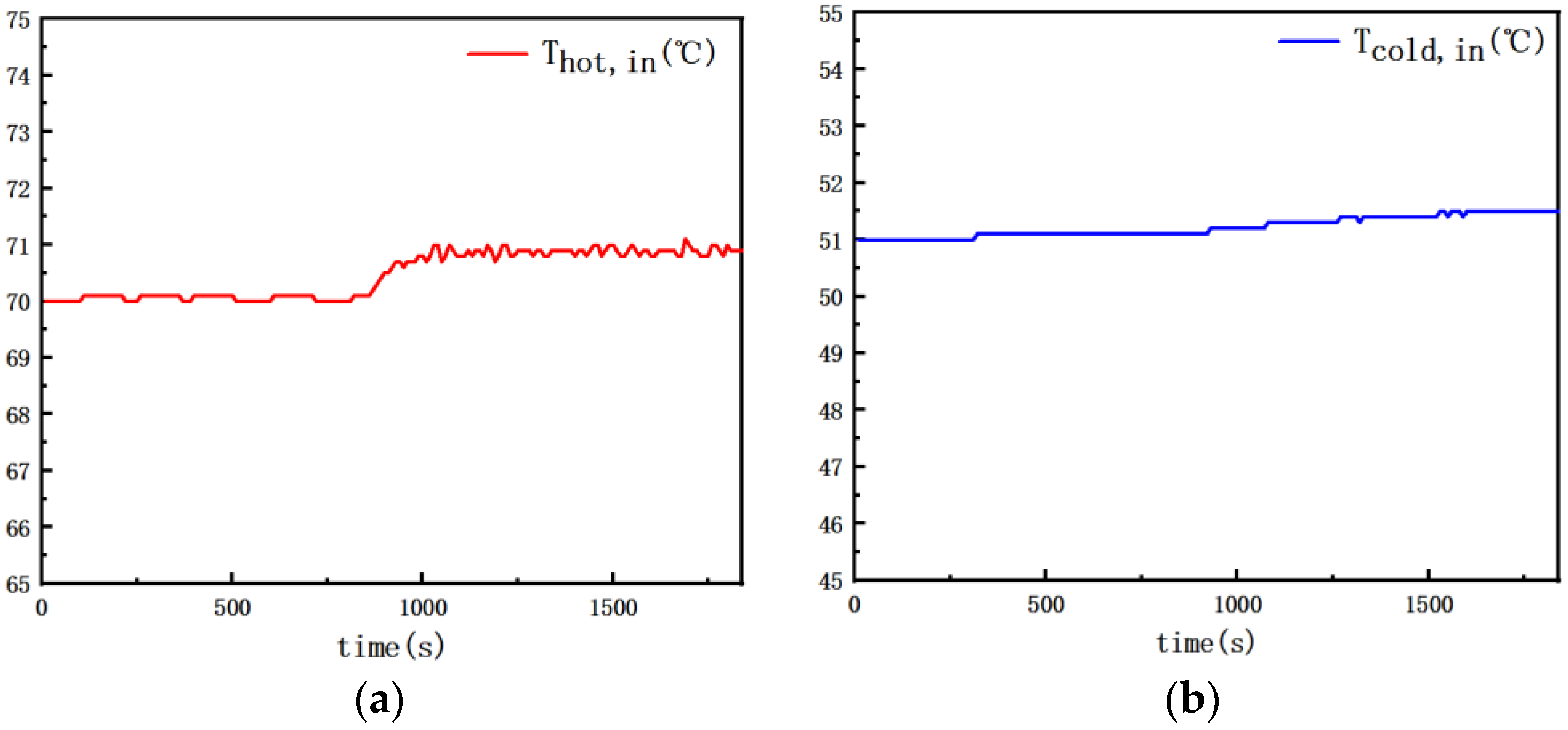
Figure 8 depicts the fluctuation in the inlet temperatures for Dataset 1, with the hot fluid side’s inlet temperature set at 70 °C. In Figure 8a, a marginal increase in the temperatures on the hot fluid side is observed as the flow rate decreases. This phenomenon is attributed to the composition of the heat source, which comprises a hot water tank and a heater operating at peak efficiency. Consequently, despite a decrease in the flow rate, the heater’s efficiency remains constant, leading to an elevation in the temperature of the hot water tank, and consequently, the inlet temperature on the hot fluid side, where the temperature is around 71 degrees. Simultaneously, the inlet temperature on the cold fluid side experiences a corresponding increase, and the temperature is around 52 degrees.
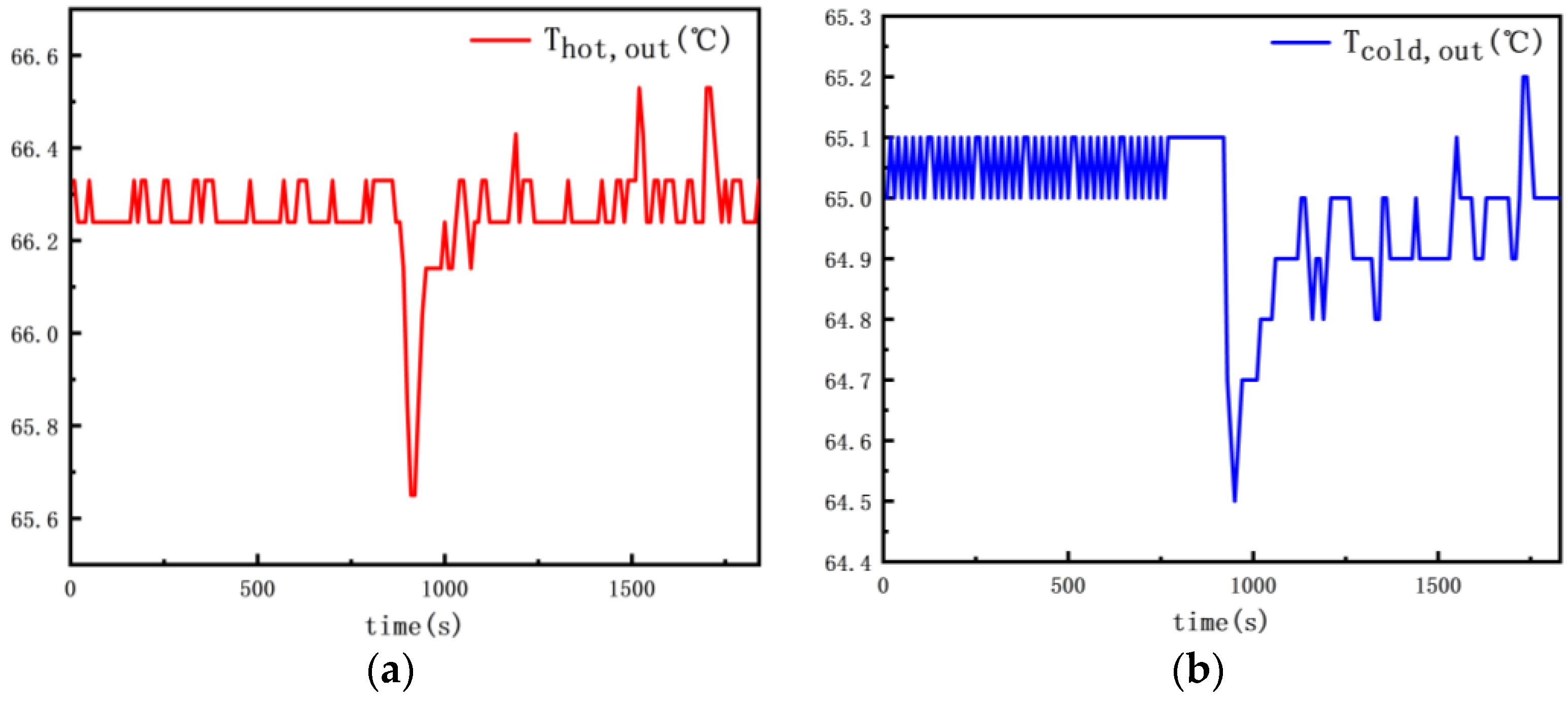
In Figure 9 for Dataset 1, the variation in outlet temperatures on both sides is depicted. With a decrease in the flow rate, the total heat remains constant over a short period, leading to an increase in the temperature difference. Consequently, the outlet temperature on the hot fluid side decreases. Subsequently, as heat diminishes, the temperature difference decreases, causing an elevation in the outlet temperature on the hot fluid side. Due to lag, the outlet temperature on the cold fluid side experiences a delayed response compared to the changes observed on the hot fluid side during this time interval.
Figure 10 illustrates the variation in the hot fluid side flow rate for Dataset 2, where the flow rate changes from 0.69 m³/h to 0.93 m³/h, while the flow rate on the cold fluid side remains constant at 0.18 m³/h.
Figure 11 depicts the variation in the inlet temperatures for Dataset 2. In the scenario where the flow rate on the hot fluid side increases, Figure 11a shows a decrease in the inlet temperature on the hot fluid side, followed by a slow upward trend. This is attributed to the insufficient power of the heater, which cannot provide high-power heating for an extended period, leading to a situation where the inlet temperature on the hot fluid side cannot be maintained at 70 °C. Similarly, the inlet temperature on the cold fluid side continues to rise due to the sustained heating by the heater.
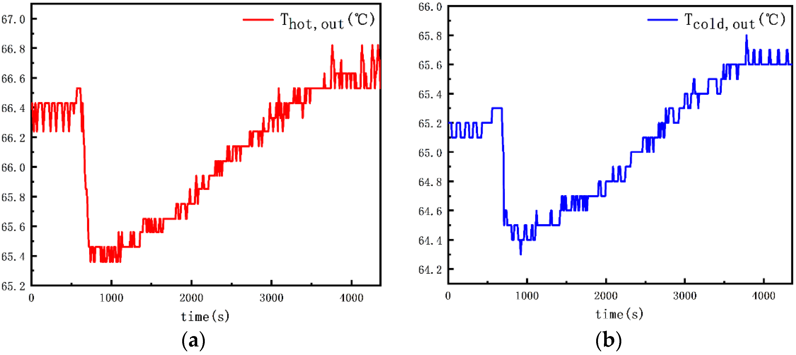
Figure 12 illustrates the variations in outlet temperatures for Dataset 2. The increase in the flow rate on the hot fluid side results in a significant decrease in the outlet temperature across the entire hot fluid side pipeline. As the inlet temperature on the hot fluid side rises, the outlet temperature on the hot fluid side gradually increases. A similar trend is observed for the outlet temperature on the cold fluid side.
3.2. Training Results of the New Model
3.2.1. Dataset Results Analysis
Under the guidance of the real-time operation results of the heat exchanger, reinforcement learning is employed to train the two sets of data based on the new heat exchanger model. For the first dataset, 184 sets of effective data were trained, achieving a maximum accumulated reward of 1540. According to the reward function (16), if the relative errors of all data are less than 0.05, the maximum accumulated reward would be 1840. If all data have relative errors less than 0.1, a minimum accumulated reward of 920 can be obtained. The attainment of a maximum reward value of 1540 indicates satisfactory training results with a high level of precision. This is also the reason for setting the training rounds to 1000. The quality of the training results depends on the number of training rounds, suggesting that there is still room for improvement in achieving a higher maximum cumulative reward.
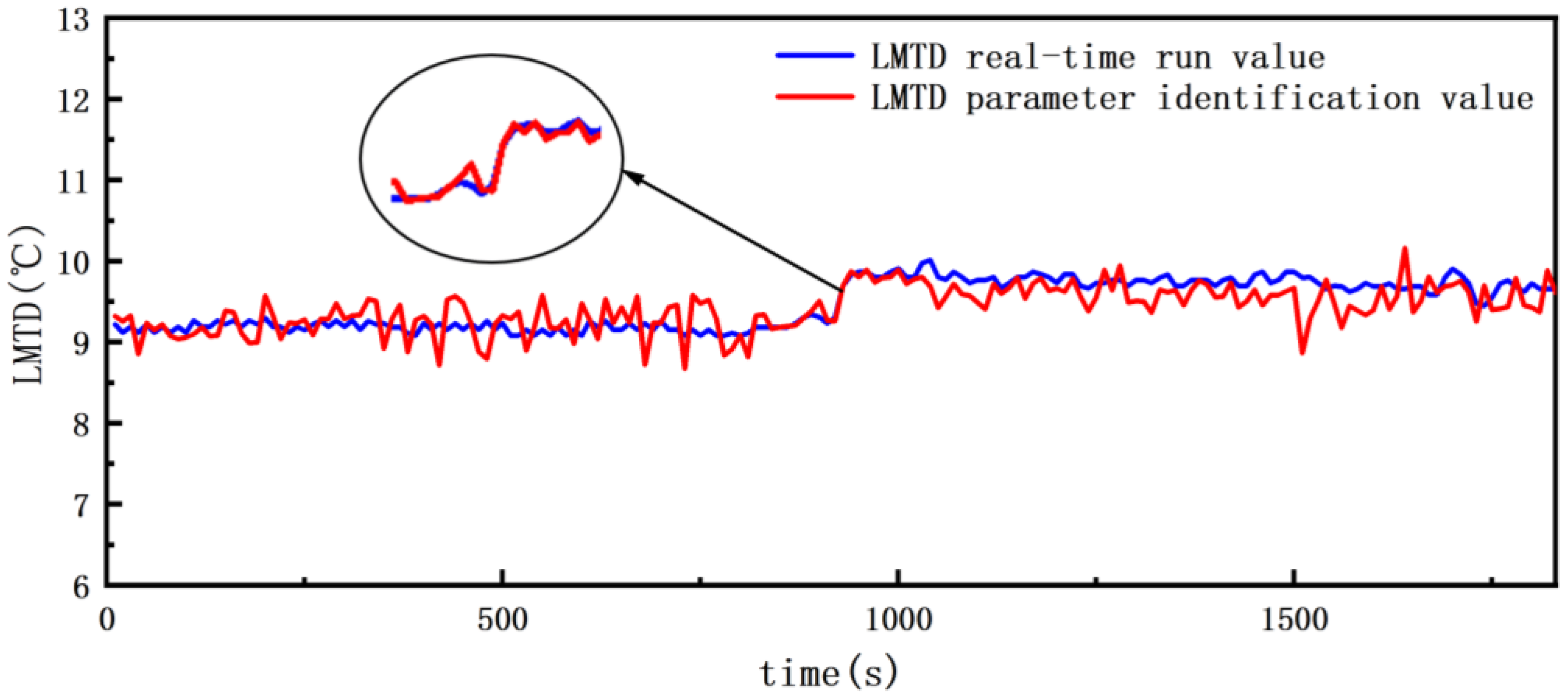
Figure 13 compares the model output results of the reinforcement learning parameter identification method for Dataset 1 with the real-time operation data. It can be observed that the LMTD values in both situations are very close, with a minimum difference of 0.85 °C. The LMTD remains in a stable fluctuation state before the change in flow rate. After the flow rate decreases, the LMTD slowly rises and then stabilizes in a fluctuating state. The results identified by the reinforcement learning method are distributed around the real-time operation data. The intelligent agent continuously explores by maximizing the accumulated reward, recording values that satisfy the reward function. Values with a better exploration than the previous step’s exploration are replaced, and the exploration amplitude of actions varies, causing the LMTD parameter identification values to fluctuate continuously. This is a normal exploration path for the agent’s actions. The LMTD is a comprehensive temperature indicator. From a physical perspective, when the heat fluid flow rate suddenly decreases within a very short period, due to the thermal inertia of the temperature, the heat on the heat fluid side remains constant for a short time. After the flow rate abruptly changes, the outlet temperature of the heat fluid starts to decrease, leading to an increase in the temperature difference on the heat fluid side. As time passes, the heat decreases, and the flow stabilizes. Hence, the temperature difference on the heat fluid side decreases. After the heat stabilizes, the outlet temperature begins to rise, and once the heat stabilizes, the outlet temperature also stabilizes. Therefore, the LMTD tends to be in a stable fluctuating state. From this, it can be observed that the new model parameter identification process has a clear physical significance and interpretability support.
In order to validate the scalability and applicability of the new model parameter identification, Dataset 2, which had an increase in the hot-side flow rate, was selected. Dataset 2 obtained a total of 336 valid data points, achieving a maximum cumulative reward of 2950. If all valid data points have a relative error less than 0.05, the maximum cumulative reward would be 3360. From the perspective of identification reward values, the K values identified through reinforcement learning parameter identification in the new heat exchanger model exhibit an extremely high precision. Figure 14 compares the output results of the reinforcement learning parameter identification method in Dataset 2 with the real-time operating data. With an increase in the hot fluid flow rate, the LMTD decreases in the short term, then gradually rises with a slow trend, and finally stabilizes within a small fluctuation range, continuously oscillating. The sudden increase in the heat flux causes the hot fluid inlet temperature to not reach the set fixed value, leading to a decrease. This is also the reason for the short-term decrease in the LMTD. As time progresses, the inlet temperature will gradually increase to reach the set temperature value, causing the LMTD to slowly rise. The identified parameter values align with their physical meanings. This indicates that the model has good scalability and applicability under different real-time operating data, suitable for all flow rate variation operational data.
The identification results from the two datasets, as indicated by the maximum accumulated reward during training and the figures, demonstrate a high level of accuracy in the reinforcement learning for this model. The average relative errors were calculated, resulting in 2.7% for Dataset 1 and 2.9% for Dataset 2. Both training sets exhibit an identification accuracy within 5%. This confirms that the new model achieves a high precision in identifying the parameter K, meeting the accuracy requirements for the precise control of the K value.
3.2.2. Verification Analysis of Overall Heat Transfer Coefficient K
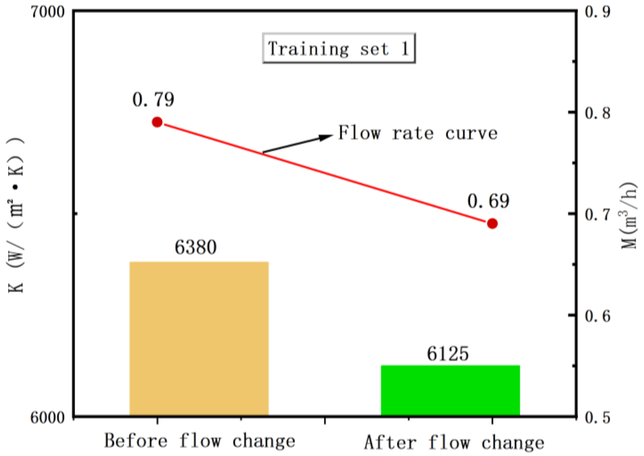
Using reinforcement learning techniques on the new heat exchanger model, the total heat transfer coefficient K is subjected to parameter identification. The identified values of K are then utilized to validate the effectiveness of the dataset, paving the way for the precise control of the heat exchange system in the subsequent stages. The real-time operational data are collected before and after the change in the heat flow rate. Therefore, the identified values of the total heat transfer coefficient K at these two instances are chosen for validation. Figure 15 illustrates the variation in the identified values of the total heat transfer coefficient K obtained through model parameter identification when the heat flow rate decreases in Dataset 1. As the flow rate decreases, the overall heat transfer in the heat exchanger system decreases, leading to a reduction in the heat transfer capacity of the heat exchanger. Consequently, the K value also decreases, aligning with the physical interpretation of the flow rate variation. Figure 16 depicts the increase in the identified values of the total heat transfer coefficient K in Dataset 2 when the heat flow rate on the hot side increases. In this scenario, the identified K value increases after training, as the higher flow rate enhances the heat transfer capacity of the heat exchanger. The accurate identification of the K values by the model demonstrates its precision, laying the foundation for the precise identification of dynamic parameters before achieving accurate control in subsequent heat exchanger system model predictions.
3.3. Further Exploration of Identification Accuracy Improvement
The new heat exchanger model has already demonstrated a high level of identification accuracy. However, aiming for further improvement in its identification precision, the authors introduce a new reward function based on the arithmetic mean temperature difference (AMTD). In contrast to the previous reinforcement learning, which utilized the relative error between the model’s output LMTD identification value and the calculated LMTD value from operational data, the authors investigate the potential enhancement in the model identification accuracy through the utilization of the AMTD. From the perspective of the reward function, the selection of parameters in the reward function is directly related to the operating parameters of the heat exchanger unit. Therefore, we only consider the parameter selection under temperature and flow rate conditions. From the perspective of the operating principle of the heat exchanger, the flow rate, as an actively controlled state variable, cannot be chosen. If only the outlet temperature of one side is selected, the results are not comprehensive. Therefore, we considered the comprehensive capabilities of average temperature differences such as the AMTD or LMTD. Thus, a comparative study was conducted on the AMTD and LMTD. The expression for AMTD is:
A comparative analysis of the identification performance under the two reward functions is conducted using standard deviation, relative error, and average relative error metrics. Figure 17 represents the standard deviation values of the identification results and data values for the two training sets. The shaded areas depict the standard deviation between the identification values and the data values, where a smaller shaded area indicates a smaller standard deviation. The graph indicates that using the relative error based on the AMTD as the reward function results in a smaller shaded area compared to using the relative error based on the LMTD as the reward function. From the perspective of standard deviation, this suggests that the former, relying on the new model, exhibits a higher identification accuracy than the latter. References [36,37] indicate that reducing the complexity of the dataset can potentially improve the accuracy of deep learning models. In future research, we will further consider the impact of data complexity on the model.
Based on the analysis of the standard deviation, the authors further compare the two using relative error values, as shown in Figure 18. The relative error ranges for both are within 10%, and the fluctuation in the relative error is attributed to the same reasons as the fluctuation in the identification results. To achieve better reward results more quickly, a relatively large exploration amplitude was set. The identification accuracy already meets the basic requirements of the heat exchanger. If more stable identification errors are desired, a longer exploration with a smaller exploration amplitude can be conducted. The results in the figure indicate that the settling rate near zero values using the AMTD relative error as the reward function is higher than the settling rate with the other reward function. This suggests that this reward function is more adaptable to the model than the other. Finally, both are analyzed based on their average relative error. Using the LMTD relative error as the reward function results in average relative error values of 2.7% and 2.9%, while using the AMTD relative error as the reward function yields average relative error values of 2.26% and 2.64%. The comparative analysis using three numerical methods suggests that under the given operating conditions, using the AMTD relative error as the reward function leads to a higher match with the model, with an average relative error within 5%, indicating an extremely high identification accuracy.
The exploration of the model’s identification accuracy has been completed in this paper. Through the analysis of the training set, the new model demonstrates a clear physical significance and exhibits good scalability and applicability to different operating data. The application of reinforcement learning for parameter identification based on the new model shows a high identification accuracy. Furthermore, the comparison of different reward functions with the model’s match and identification accuracy has been conducted. The training results indicate that using the AMTD relative error as the reward function leads to a higher model match and identification accuracy compared to using the LMTD relative error as the reward function.
This study conducted parameter identification for the overall heat transfer coefficient K of plate heat exchangers. Traditional models were unable to identify the real-time K value of plate heat exchangers in the heat exchange system solely based on the temperature and flow rate values. We addressed this issue by combining mechanistic modeling with reinforcement learning. Similarly, it has provided significant assistance in addressing the lack of high-precision models for control and optimization problems in heat exchange system operations. The identification of the overall heat transfer coefficient K serves as one of the indicators for evaluating heat exchanger performance. It is directly related to various heat exchange performance indicators through equations, such as the thermal resistance defined by heat dissipation. There exists a certain nonlinear relationship between the two. By accurately identifying the K value, we can determine the current state’s thermal resistance defined by heat dissipation. According to the principle of minimizing thermal resistance defined by heat dissipation, the lower the thermal resistance defined by heat dissipation, the higher the operational efficiency of the heat exchange system. This facilitates optimal control by identifying the most efficient coupling point of the flow rate and temperature under system operation, enabling equipment regulation. Therefore, the precise identification of K becomes the implementation basis for the operation and control of heat exchange systems.
4. Conclusions and Future Work
4.1. Conclusions
A modeling approach based on the collaboration of mechanisms and data for heat exchangers is proposed. Due to the challenge of obtaining accurate real-time K values in the heat exchanger, reinforcement learning is introduced for the parameter identification of the heat transfer coefficient K based on operational data. The accuracy of the model and the identification precision under different reward functions are compared. The results are as follows:
- Under the collaborative mechanism and data driving of the heat exchanger model, the average relative error of the identified values obtained through parameter identification is within 5%, demonstrating a high level of identification accuracy. This heat exchanger modeling approach proves to be highly applicable, and the comparisons under various operating conditions reflect the model’s versatility and physical relevance.
- Due to the adoption of two temperature differences as reward functions in this paper, and since the reward function is only related to the temperature values, the control of the flow rate only considered operating condition changes in the hot-side flow rate. In the comparison under various operating conditions, using the relative error of the AMTD as the reward function showed a higher matching degree and identification accuracy compared to using the relative error of the LMTD as the reward function.
- Proposing the method of using reinforcement learning for parameter identification of the real-time heat transfer coefficient K in heat exchanger units, the identified K values lay the theoretical foundation for the precise control of the heat exchange system. Moreover, based on these results, model predictive control can be applied to achieve control optimization of the system operation.
4.2. Future Work
Intelligent heating in the HVAC field has always been an industry goal, with the key challenges being precise heating and on-demand heating. Identifying the real-time operating heat transfer coefficient K is just the first step. There is still significant room for improvement in applying the real-time variation of coefficients to the control of heat exchange systems. We believe that Model Predictive Control (MPC) is an intelligent cornerstone in the future of HVAC control. The losses and risks brought about by manual regulation need to be completely eliminated. The research model on the identification of K is just a foundation for achieving intelligent HVAC control. The real challenge in the future of HVAC control is to integrate dynamic model identification with automatic device regulation based on the system’s state. Currently, only by thoroughly understanding the theoretical research underpinning the heat transfer mechanism can we make the application of Model Predictive Control more convenient. This represents both a challenge and an opportunity in the future of HVAC control strategies.
Author Contributions
Conceptualization, H.S. and Z.J.; Methodology, H.S. and Z.J.; Software, H.S. and Z.J.; Validation, H.S. and Z.J.; Formal analysis, H.S. and M.Z.; Investigation, H.S., D.L. and J.T.; Data curation, H.S., D.L. and J.T.; Writing—original draft, H.S.; Writing—review and editing, H.S., Y.W. and M.Z.; Visualization, H.S. and J.T.; Supervision, Z.J.; Project administration, M.Z. and Z.J.; Funding acquisition, Z.J and M.Z. All authors have read and agreed to the published version of the manuscript.
Funding
This study was funded by the Inner Mongolia Natural Science Foundation of China (2023LHMS01010), Inner Mongolia Higher Education Scientific Research Project of China (NJZY21335), and Ungar Science and Technology Program of China (2023YY-20).
Data Availability Statement
The XLSX data used to support the findings of this study may be accessed by emailing to the corresponding author. The available time will be six months after the publication since there are still some researches and articles for submission based on this manuscript and the original data.
Conflicts of Interest
The authors declare no conflicts of interest.
References
- International Energy Agency (IEA). Energy Efficiency 2020. 2020. Available online: https://www.iea.org/reports/energy-efficiency-2020 (accessed on 15 March 2024).
- Shahnazari, H.; Mhaskar, P.; House, J.M.; Salsbury, T.I. Heating, ventilation and air conditioning systems: Fault detection and isolation and safe parking. Comput. Chem. Eng. 2018, 108, 139–151. [Google Scholar] [CrossRef]
- Suhendri, S.; Hu, M.; Dan, Y.; Su, Y.; Zhao, B.; Riffat, S. Building energy-saving potential of a dual-functional solar heating and radiative cooling system. Energy Build. 2024, 303, 113764. [Google Scholar] [CrossRef]
- Chen, F.; Jiang, X.; Lu, C.; Wang, Y.; Wen, P.; Shen, Q. Heat transfer efficiency enhancement of gyroid heat exchanger based on multidimensional gradient structure design. Int. Commun. Heat Mass Transf. 2023, 149, 107127. [Google Scholar] [CrossRef]
- Ali, S.; Faraj, J.; Awad, S.; Ramadan, H.S.; Khaled, M.; Dbouk, T. Innovative algorithmic approach of determining the overall heat transfer coefficient of concentric tube heat exchangers. Int. Commun. Heat Mass Transf. 2023, 148, 107077. [Google Scholar] [CrossRef]
- Li, W.-T.; Tushar, W.; Yuen, C.; Ng, B.K.K.; Tai, S.; Chew, K.T. Energy efficiency improvement of solar water heating systems—An IoT based commissioning methodology. Energy Build. 2020, 224, 110231. [Google Scholar] [CrossRef]
- Li, Z.; Liu, J.; Jia, L.; Wang, Y. Improving room temperature stability and operation efficiency using a model predictive control method for a district heating station. Energy Build. 2023, 287, 112990. [Google Scholar] [CrossRef]
- Zhuang, D.; Gan, V.J.; Tekler, Z.D.; Chong, A.; Tian, S.; Shi, X. Data-driven predictive control for smart HVAC system in IoT-integrated buildings with time-series forecasting and reinforcement learning. Appl. Energy 2023, 338, 120936. [Google Scholar] [CrossRef]
- Jiang, Z.; Risbeck, M.J.; Ramamurti, V.; Murugesan, S.; Amores, J.; Zhang, C.; Lee, Y.M.; Drees, K.H. Building HVAC control with reinforcement learning for reduction of energy cost and demand charge. Energy Build. 2021, 239, 110833. [Google Scholar] [CrossRef]
- Smith, J.; Wang, L. Advances in Heat Exchanger Technology. J. Therm. Sci. 2018, 27, 307–322. [Google Scholar]
- Gao, Y.; Tian, Q.; Wu, B.; Dong, X.; Wang, Y. Mathematical Modeling and Simulation of Heat Transfer Performance in Solar/Air Energy Collector-Evaporator. Acta Energiae Solaris Sin. 2020, 41, 57–63. [Google Scholar]
- Chen, H.; Zhang, W. Real-time Monitoring of Heat Exchanger Performance Using Data-driven Methods. Energy Procedia 2017, 105, 456–461. [Google Scholar]
- Cao, Y. Operation Evaluation and Energy Saving Potential Analysis of Heat Exchange Station Based on Data Modeling; Tianjin University: Tianjin, China, 2020. [Google Scholar]
- Zhong, L. Research on Modeling and Control Algorithm of MPCE Experimental Device Column Heat Exchanger System; Central South University: Changsha, China, 2011. [Google Scholar]
- Lu, G.; Wang, Y.; You, S. Research on Dynamic Modeling and System Identification of Heating System. Dist. Heat. 2021, 16–22. [Google Scholar] [CrossRef]
- Wang, Z.; Wu, Z. Nonlinear Modeling and Identification of Heat Exchanger Systems. Control Eng. Pract. 2016, 52, 78–89. [Google Scholar]
- Miao, Q.; You, S.; Zheng, W.; Zheng, X.; Zhang, H.; Wang, Y. A Grey-Box Dynamic Model of Plate Heat Exchangers Used in an Urban Heating System. Energies 2017, 10, 1398. [Google Scholar] [CrossRef]
- Dong, S.; Wang, K.; Gao, H.; Wang, J. Three-Element Linear Regression Model and Coefficient Identification of Plate-Fin Heat Exchanger Heat Transfer Performance. J. Aeronaut. 2012, 33, 1571–1577. [Google Scholar]
- Zhao, X.; Li, N. Online Diagnosis and Selective Control Analysis of Heat Exchanger Leakage Abnormal Condition Based on Least Squares Method. Appl. Chem. Ind. 2020, 49, 312–316. [Google Scholar]
- Wang, Z.; Zhou, Z.; Xu, W.; Sun, C.; Yan, R. Physics informed neural networks for fault severity identification of axial piston pumps. J. Manuf. Syst. 2023, 71, 421–437. [Google Scholar] [CrossRef]
- Zhou, S. System Identification and Control Based on Neural Networks; North China Electric Power University (Beijing): Beijing, China, 2017. [Google Scholar]
- Yuan, Y. Permanent Magnet Synchronous Motor Parameter Identification Based on Adaptive Particle Swarm Optimization Algorithm. Meas. Control Technol. 2018, 37, 42–45+13. [Google Scholar]
- Zheng, Y.; Hu, G.; Zhang, Z. Robust Parameter Identification Method for Photovoltaic Array Model Based on Genetic Algorithm and Nonlinear Programming. Comput. Meas. Control 2021, 29, 189–193. [Google Scholar]
- Wang, R.; Wang, P. Steady-State Modeling and Parameter Estimation of Isolated Heat Pipe Heat Transfer Energy-Saving System. J. Beijing Univ. Technol. 2013, 39, 835–839. [Google Scholar]
- Wan, M.; Ying, Z.; Zhang, X. Study on Power Device Aggregate Parameter Thermal Circuit Model and Parameter Extraction. Trans. China Electrotech. Soc. 2015, 30, 31–38. [Google Scholar]
- Solinas, F.M.; Macii, A.; Patti, E.; Bottaccioli, L. An online reinforcement learning approach for HVAC control. Expert Syst. Appl. 2024, 238, 121749. [Google Scholar] [CrossRef]
- Wang, H.; Wang, Y.; Lu, Y.; Fu, Q.; Chen, J. Visual interpretation of deep deterministic policy gradient models for energy consumption prediction. J. Build. Eng. 2023, 79, 107847. [Google Scholar] [CrossRef]
- Hartman, L.B.; van Hee, K.M. Application of Markov decision processes to search problems. Decis. Support Syst. 1995, 14, 283–298. [Google Scholar] [CrossRef]
- Xu, B.; Li, X. A Q-learning based transient power optimization method for organic Rankine cycle waste heat recovery system in heavy duty diesel engine applications. Appl. Energy 2021, 286, 116532. [Google Scholar] [CrossRef]
- Kim, Y.T.; Han, S.Y. Cooling channel designs of a prismatic battery pack for electric vehicle using the deep Q-network algorithm. Appl. Therm. Eng. 2023, 219, 119610. [Google Scholar] [CrossRef]
- Dong, Y.; Zhang, H.; Wang, C.; Zhou, X. Soft actor-critic DRL algorithm for interval optimal dispatch of integrated energy systems with uncertainty in demand response and renewable energy. Eng. Appl. Artif. Intell. 2024, 127, 107230. [Google Scholar] [CrossRef]
- Lillicrap, T.P.; Hunt, J.J.; Pritzel, A.; Heess, N.; Erez, T.; Tassa, Y.; Silver, D.; Wierstra, D. Continuous control with deep reinforcement learning. arXiv 2015, arXiv:1509.02971. [Google Scholar]
- Shixiang, G.U.; Lillicrap, T.P.; Sutskever, I.; Levine, S.V. Reinforcement Learning Using Advantage Estimates. U.S. Patent US11288568B2, 23 December 2023. [Google Scholar]
- Haarnoja, T.; Zhou, A.; Abbeel, P.; Levine, S. Soft Actor-Critic: Off-Policy Maximum Entropy Deep Reinforcement Learning with a Stochastic Actor. In Proceedings of the 35th International Conference on Machine Learning, Stockholm, Sweden, 10–15 July 2018. [Google Scholar]
- Fujimoto, S.; Van Hoof, H.; Meger, D. Addressing Function Approximation Error in Actor-Critic Methods. In Proceedings of the 35th International Conference on Machine Learning, Stockholm, Sweden, 10–15 July 2018. [Google Scholar]
- Bolón-Canedo, V.; Remeseiro, B. Feature selection in image analysis: A survey. Artif. Intell. Rev. 2020, 53, 2905–2931. [Google Scholar] [CrossRef]
- Kabir, H.; Garg, N. Machine learning enabled orthogonal camera goniometry for accurate and robust contact angle measurements. Sci. Rep. 2023, 13, 1497. [Google Scholar] [CrossRef] [PubMed]
Figure 1.
Framework diagram.

Figure 2.
Schematic diagram of the exchange system.

Figure 3.
2-sigma preprocessing of outlier values.

Figure 4.
Preprocessing of missing values using the moving average method.

Figure 5.
Heat exchanger parameter identification method based on reinforcement learning.

Figure 6.
DDPG algorithm framework.

Figure 7.
Variation of hot fluid flow rate in Dataset 1.

Figure 8.
Temperature variation at both inlets for Dataset 1. (a) Hot-side inlet temperature variation; (b) cold-side inlet temperature variation.
Figure 8.
Temperature variation at both inlets for Dataset 1. (a) Hot-side inlet temperature variation; (b) cold-side inlet temperature variation.

Figure 9.
Temperature variation at both outlets for Dataset 1. (a) Hot-side outlet temperature variation; (b) cold-side outlet temperature variation.
Figure 9.
Temperature variation at both outlets for Dataset 1. (a) Hot-side outlet temperature variation; (b) cold-side outlet temperature variation.

Figure 10.
Hot-side flow rate variation for Dataset 2.

Figure 11.
Temperature variation at both inlets for Dataset 2. (a) Hot-side inlet temperature variation; (b) cold-side inlet temperature variation.
Figure 11.
Temperature variation at both inlets for Dataset 2. (a) Hot-side inlet temperature variation; (b) cold-side inlet temperature variation.

Figure 12.
Temperature variation at both outlets for Dataset 2. (a) Hot-side outlet temperature variation; (b) cold-side outlet temperature variation.
Figure 12.
Temperature variation at both outlets for Dataset 2. (a) Hot-side outlet temperature variation; (b) cold-side outlet temperature variation.

Figure 13.
Comparison of parameter identification values from Dataset 1 with real-time operating values.
Figure 13.
Comparison of parameter identification values from Dataset 1 with real-time operating values.

Figure 14.
Comparison between the identified parameter values and real-time operating values in Dataset 2.
Figure 14.
Comparison between the identified parameter values and real-time operating values in Dataset 2.

Figure 15.
Validation of parameter identification for K in Dataset 1.

Figure 16.
Validation of parameter identification for K in Dataset 2.

Figure 17.
Comparison of standard deviation values. (a) Comparison of standard deviation values in Dataset 1; (b) comparison of standard deviation values in Dataset 2.
Figure 17.
Comparison of standard deviation values. (a) Comparison of standard deviation values in Dataset 1; (b) comparison of standard deviation values in Dataset 2.

Figure 18.
Comparison of relative errors. (a) Comparison of relative errors in Dataset 1; (b) comparison of relative errors in Dataset 1.
Figure 18.
Comparison of relative errors. (a) Comparison of relative errors in Dataset 1; (b) comparison of relative errors in Dataset 1.


Table 1.
Main parameters and accuracy of system devices.
| Device Name and Manufacturer | Main Parameters and Precision of the System Setup | |
|---|---|---|
 | Plate heat exchanger Shouguang city, China, Yuanxing machinery and equipment | Heat exchange area: 0.2 m2 Maximum operating temperature: 160 °C Maximum operating pressure: 1.5 MPa |
 | Primary network electric heater Yangzhou city, China, electric power equipment | Power: 6 KW Operating voltage: 220 V Rated pressure: 1.0 MPa |
 | Mitsubishi E700 inverter Suzhou city, China, Xicheng environmental protection technology | Frequency range: 0~50 Hz Instrument capacity: 3.7 KW Instrument accuracy: 0.01 Hz |
 | Primary network pump Shanghai city, China, Sunshine pump | Flow rate: 18 m3/h Power: 4 KW Efficiency: 55% |
 | Secondary network pump Shanghai city, China, Sunshine pump | Flow rate: 16 m3/h Power: 4 KW Efficiency: 55% |
 | Flow meter Shouguang city, China, Jebsen Instrument automation equipment | Operating temperature range: −20 °C~100 °C Measurement accuracy: ±0.5% |
 | Temperature sensor Nanjing city, China, On the automatic instrument | Operating temperature range: −50 °C~200 °C Measurement accuracy: ±3% |
Table 2.
The update steps for the DDPG algorithm.
| Steps | Algorithm Update Process |
|---|---|
| Step 1 | Randomly extract state transition data (st, at, rt, st + 1) from the database |
| Step 2 | The actor provides at+ 1 to the critic based on st+1 |
| Step 3 | The critic calculates Q (st, at) and Q (st + 1, at + 1) based on (st, at) and (st + 1, at + 1), then computes the TD (Temporal Difference) error |
| Step 4 | The critic updates the weight parameters based on the TD error |
| Step 5 | The actor updates the weight parameters based on the Q (st, at) provided by the critic |
Table 3.
Hyperparameter settings.
| Parameter | Value |
|---|---|
| Actor learning rate | 3 × 10⁻⁴ |
| Critic learning rate | 3 × 10⁻³ |
| Training epochs | 1000 |
| Discount factor | 0.98 |
| Experience replay buffer size | 10,000 |
| Neural network hidden dimension | 64 |
| Soft update parameter | 0.001 |
| Minimum stored experiences in the experience replay buffer | 1000 |
| Sample size per extraction | 64 |
| Gaussian noise standard deviation | 100 |
Disclaimer/Publisher’s Note: The statements, opinions and data contained in all publications are solely those of the individual author(s) and contributor(s) and not of MDPI and/or the editor(s). MDPI and/or the editor(s) disclaim responsibility for any injury to people or property resulting from any ideas, methods, instructions or products referred to in the content. |
© 2024 by the authors. Licensee MDPI, Basel, Switzerland. This article is an open access article distributed under the terms and conditions of the Creative Commons Attribution (CC BY) license (https://creativecommons.org/licenses/by/4.0/).
Share and Cite
MDPI and ACS Style
Sun, H.; Jia, Z.; Zhao, M.; Tian, J.; Liu, D.; Wang, Y. Dynamic Modeling of Heat Exchangers Based on Mechanism and Reinforcement Learning Synergy. Buildings 2024, 14, 833. https://0-doi-org.brum.beds.ac.uk/10.3390/buildings14030833
AMA Style
Sun H, Jia Z, Zhao M, Tian J, Liu D, Wang Y. Dynamic Modeling of Heat Exchangers Based on Mechanism and Reinforcement Learning Synergy. Buildings. 2024; 14(3):833. https://0-doi-org.brum.beds.ac.uk/10.3390/buildings14030833
Chicago/Turabian StyleSun, Hao, Zile Jia, Meng Zhao, Jiayuan Tian, Dan Liu, and Yifei Wang. 2024. "Dynamic Modeling of Heat Exchangers Based on Mechanism and Reinforcement Learning Synergy" Buildings 14, no. 3: 833. https://0-doi-org.brum.beds.ac.uk/10.3390/buildings14030833
Note that from the first issue of 2016, this journal uses article numbers instead of page numbers. See further details here.